| Issue |
A&A
Volume 692, December 2024
|
|
|---|---|---|
| Article Number | L9 | |
| Number of page(s) | 5 | |
| Section | Letters to the Editor | |
| DOI | https://doi.org/10.1051/0004-6361/202452741 | |
| Published online | 16 December 2024 | |
Stellar halos of bright central galaxies
A view from the FEGA semi-analytic model of galaxy formation and VEGAS survey
1
Department of Astronomy and Yonsei University Observatory, Yonsei University, 50 Yonsei-ro, Seodaemun-gu, Seoul 03722, Republic of Korea
2
INAF Osservatorio Astronomico di Capodimonte, Salita Moiariello 16, 80131 Napoli, Italy
⋆ Corresponding author; This email address is being protected from spambots. You need JavaScript enabled to view it.
Received:
25
October
2024
Accepted:
24
November
2024
Abstract
Aims. We present theoretical predictions and extrapolations from observed data of the stellar halos surrounding central group and cluster galaxies, and the transition radius between them and the intracluster or diffuse light.
Methods. Leveraging the state-of-the-art semi-analytic model of galaxy formation, FEGA (Formation and Evolution of GAlaxies), applied to two dark matter-only cosmological simulations, we derived both the stellar halo mass and its radius. Using theoretical assumptions about the diffuse light distribution and halo concentration, we extrapolated the same information for observed data from the VEGAS survey.
Results. Our model, supported by observational data and independent simulation results, predicts an increasing transition radius with halo mass, a constant stellar halo-to-intracluster light ratio, and a stable stellar halo mass fraction with increasing halo mass. Specifically, we find that the transition radius between the stellar halo and the diffuse light ranges from 20 to 250 kpc, from Milky Way-like halos to large clusters, while the stellar halo mass comprises only a small fraction, between 7% and 18%, of the total stellar mass within the virial radius.
Conclusions. These results support the idea that the stellar halo can be viewed as a transition region between the stars bound to a galaxy and those belonging to the intracluster light and are consistent with recent observations and theoretical predictions.
Key words: galaxies: evolution / galaxies: formation
© The Authors 2024
 Open Access article, published by EDP Sciences, under the terms of the Creative Commons Attribution License (https://creativecommons.org/licenses/by/4.0), which permits unrestricted use, distribution, and reproduction in any medium, provided the original work is properly cited.
This article is published in open access under the Subscribe to Open model. This email address is being protected from spambots. You need JavaScript enabled to view it. to support open access publication.
1. Introduction
Stellar halos (SHs) are extended, diffuse regions of stars that surround the central parts of galaxies, such as the bulge and disk (for a review, see Arnaboldi & Gerhard 2022). Composed mainly of old metal-poor stars, these halos provide crucial insights into the formation history of galaxies (Helmi 2008; Iodice et al. 2016; Helmi et al. 2018). The stars in stellar halos are believed to originate from ancient dwarf galaxies that were accreted by the host galaxy through gravitational interactions (Helmi et al. 1999; Bullock & Johnston 2005; Lane et al. 2022; Duc et al. 2015) or from early star formation during the galaxy’s initial phases of evolution (Helmi 2008). Unlike stars in the galactic disk, which follow ordered circular orbits, SH stars are distributed in random, highly elliptical trajectories (Helmi 2020). The extent of SHs can reach up to several hundred kiloparsecs in the most massive galaxies, providing a glimpse into past mergers and accretion events that shaped their evolution (Helmi et al. 2018).
The stars coming from dwarf galaxies are the dominant channel for the formation of SHs (e.g., Cooper et al. 2010; Harmsen et al. 2017; Beltrand et al. 2024), but theoretical studies have also shown that some stars were actually formed in situ (Abadi et al. 2006; Cooper et al. 2015; Wright et al. 2024). These in situ stars typically exhibit a higher metallicity and are predominantly distributed along the major axis of the galactic disk (Pillepich et al. 2015; Monachesi et al. 2019).
Stellar halos exhibit unique properties that distinguish them from other galactic components, such as the disk and bulge. One key characteristic is their metallicity. Stars in these halos are typically metal poor (Hartke et al. 2022), indicating that they formed early in the Universe, before the interstellar medium became enriched with heavier elements from successive generations of star formation. Spavone et al. (2022), combining data from the Fornax Deep Survey and observations from the Multi Unit Spectroscopic Explorer (MUSE), also investigated the metallicity gradients of SHs and their connection to the environment, finding milder gradients in denser environments (see also Spavone et al. 2020, 2021). In terms of age, the stars in SHs are generally old, often exceeding 10 Gyr. This supports the theory that these stars are either remnants of early primitive star formation episodes or were accreted from dwarf galaxies, as previously mentioned.
Stellar halos, being largely the product of accreted stars from stripped or disrupted galaxies that merged in a hierarchical fashion, can exhibit considerable variability in their properties, often in a stochastic manner (Amorisco 2017). Two clear examples of this are the SHs of the Milky Way and its nearest neighbor, Andromeda. The Milky Way’s SH follows a broken power-law density profile (Deason et al. 2014), whereas Andromeda’s SH displays a shallower density profile extending over several kiloparsecs (e.g., Ibata et al. 2014). The stochastic nature of SH formation may significantly influence properties such as colors and metallicity, potentially linking them to the formation of diffuse light, another component that is also thought to form stochastically (Contini et al. 2023).
Despite being extensively studied theoretically through numerical simulations (references above and therein), SHs have often been considered either part of the galaxy or the diffuse light (e.g., Contini et al. 2014). In semi-analytic models, the first attempts to model their formation date back to almost two decades ago (e.g., Bullock & Johnston 2005; De Lucia & Helmi 2008; Cooper et al. 2010). In this Letter, we present a new implementation of SHs within a state-of-the-art semi-analytic model (Contini et al. 2024a), where they are treated as a transition region between the bound stars in the galaxy and the unbound stars of the diffuse light (Longobardi et al. 2015). To maintain consistency with the properties of stars observed in SHs, we assumed they primarily originate from the stripping of galaxies during the early stages of diffuse light formation. However, they are formally distinct from the diffuse light stars, as indicated by observations (e.g., D’Souza et al. 2014; Longobardi et al. 2015) when using spectroscopy, but the separation between the two components is not trivial when looking at the light profiles.
In Section 2, we detail the implementation of SH formation in our model. In Section 3, we present our analysis, showing that the transition radius between the diffuse light and SHs, defined as the typical radius of the latter, aligns well with independent measurements from simulations (Proctor et al. 2024). Finally, in Section 4, we discuss our findings and highlight the key conclusions. Throughout the rest of the paper, stellar and halo masses are corrected for h = 0.68, and the stellar masses are derived under the assumption of a Chabrier initial mass function (Chabrier 2003).
2. Methods
The semi-analytic model FEGA (Formation and Evolution of GAlaxies) was detailed in Contini et al. (2024a), and it is a state-of-the-art model that incorporates the latest prescriptions for the baryonic physics involved in galaxy formation, including a revised star formation law and a novel implementation of the positive feedback from active galactic nuclei. (For a comprehensive discussion of the model, we refer the reader to that paper.) Here, we focus on the new features introduced in this version, specifically the formation of SHs and the definition of the transition radius between SHs and the surrounding intragroup/cluster light (IGL/ICL) or diffuse light1.
Before delving into the specifics of the SH implementation, we summarize the primary mechanisms of diffuse light formation in FEGA. Diffuse light can form through three main channels: stellar stripping of satellite galaxies, mergers, and pre-processing. In FEGA, a large portion of diffuse light arises from stars that are stripped as satellites orbit within the host halo’s potential well, particularly in the densest regions, where tidal interactions are strongest (stellar stripping channel). Another significant contribution comes from mergers between the central galaxy (CG) and satellites, where violent relaxation processes redistribute part of the stellar mass into the diffuse component (merger channel). Additionally, diffuse light can form in groups and later be accreted by larger structures during assembly (pre-processing channel), though this is essentially a sub-channel, as it originates from either stellar stripping or mergers. (For more details on the specific prescriptions of each channel, we refer the reader to Contini et al. 2024a.)
We assumed the SH forms from stars belonging to the ICL that are very close to the CG. In order to do it, we needed to define a radius within which stars in the SH are distributed, a radius that hereafter we call the transition radius, Rtrans. Following Contini & Gu (2020), we assumed that at each time, the ICL follows a Navarro-Frenk-White (NFW) profile (Navarro et al. 1997) with a higher concentration than the dark matter (DM) halo in which it resides (Harris et al. 2017; Pillepich et al. 2018; Montes & Trujillo 2019; Contini et al. 2022). Specifically, under this assumption, the ICL concentration is defined as
 (1)
(1)
where R200 and Rs, DM represent the virial and scale radii of the DM halo, respectively, and Rs, ICL is the scale radius of the ICL distribution. As in Contini & Gu (2020), the parameter γ is assumed to be greater than one in order to reflect a more concentrated ICL distribution compared to the DM. From Equation (1), the scale radius of the ICL distribution can be derived as
 (2)
(2)
We assumed that Rtrans = Rs, ICL and that all the stars within this radius, at any given time, belong to the SH. This new component, composed of stars coming from the ICL, is considered as a transition between the bound stars in the galaxy and the unbound stars in the ICL. However, under certain conditions, these stars can be accreted into the galaxy. Specifically, if Rtrans is smaller than the size of the galaxy’s bulge, all the stars within it belonging to the SH are moved into this component. Additionally, a constraint is placed on the SH mass. For dynamical stability, the semi-analytic model does not allow the SH to exceed the total mass of the galaxy, and when this occurs, the excess stars are transferred to the galaxy’s disk component.
It is important to note that a semi-analytic framework does not inherently provide information about whether stars within the SH component are gravitationally bound to the CG or not; rather, this is left to the user’s interpretation. As mentioned in Section 1, observations typically consider SH stars to be bound to the CG, forming a third stellar component within it. However, in our implementation, the model’s flexibility allows the SH to be considered either as a third component of the CG (and thus bound to it) or as a subset of the diffuse light (and therefore unbound to the CG).
In Contini & Gu (2020), the parameter γ was assumed to be three in order to align with the observed CG plus ICL mass within 100 kpc, as noted by DeMaio et al. (2020) at different redshifts. In this study, we followed the same approach as in Contini et al. (2024a) for model calibration, allowing a Markov chain Monte Carlo algorithm to determine the range of values that best reproduce the observations. Consequently, we first ran FEGA on partitions of the merger trees from the DM-only cosmological simulations YS50HR and YS200 (details in Contini et al. 2023, 2024b) to constrain γ, and then we applied it to the full merger trees to construct the galaxy catalogs. Our calibration suggests that γ varies between one and approximately three, so the model for the final catalogs assumes a random value for each ICL component within this range.
To compare the model predictions with observational data, we utilized the measurements of the ICL in galaxy groups and clusters provided by Ragusa et al. (2023) from the VST Early-type GAlaxy Survey (VEGAS; Capaccioli et al. 2015; Iodice et al. 2021; the data analysis is extensively described in Ragusa et al. 2021, 2022). The sample consists of 22 objects covering the core regions of groups and clusters in the local Universe at z < 0.05 and in the halo mass range [0.4 − 26.9]⋅1013 M⊙. In this Letter, we focus on the 17 objects detailed in Ragusa et al. (2023). VEGAS is a multi-band deep-imaging survey based on observations acquired with the ESO VLT Survey Telescope (VST; for details, see Schipani et al. 2012). Data reduction was performed using the AstroWISE pipeline (details in Venhola et al. 2017 and references therein) and the VST-Tube pipeline (Capaccioli et al. 2015), which provide comparable results. For a comprehensive description of the image data reduction, we refer the reader to Capaccioli et al. (2015), Iodice et al. (2016), and Spavone et al. (2017). All 17 objects in our sample were observed in the g and r bands, with some also observed in the u and/or i bands.
These data encompass all the diffuse light, but we needed to extrapolate the SH, which we assumed to be a transition region. To address this issue, we applied the same assumption used in the model, specifically an NFW profile for the ICL distribution, in order to derive Rtrans. Unfortunately, the halo concentration is not a directly observable quantity, yet it is essential for defining Rtrans. Therefore, we utilized the halo concentration-mass relation (e.g., Prada et al. 2012; Correa et al. 2015; Child et al. 2018) from Correa et al. (2015) to derive c200 from the virial mass, and using a random γ within the same range mentioned above, we calculated cICL from Equation (1) first and finally Rtrans from Equation (2). With this information and the assumption of an NFW profile, we could isolate the light in the transition region, which we consider to be the SH in this Letter, from the ICL measurements reported by Ragusa et al. (2023).
3. Results
In this section, we proceed with the analysis, which we started by plotting, in Figure 1, the transition radius, Rtrans, as a function of the halo mass of CGs. Overlaid on our model predictions (red and blue lines2) are the independent measurements of the transition radius by Proctor et al. (2024) from the Eagle (Schaye et al. 2015; Crain et al. 2015) and C-Eagle (Bahé et al. 2017; Barnes et al. 2017) simulations (cyan, orange, and green symbols) along with our extrapolations of the observed data by Ragusa et al. (2023) from the VEGAS survey (brown symbols). With overplotted dashed (YS50HR) and solid (YS200) lines, we show the scale radius-halo mass relation.
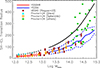 |
Fig. 1. Transition radius between the SH and the surrounding ICL as a function of halo mass. Our model predictions (red and blue lines) are compared with the results from Proctor et al. (2024) based on the Eagle (cyan and orange symbols) and C-Eagle (green symbols) simulations and extrapolations of observed data by Ragusa et al. (2023) from the VEGAS survey (brown symbols). For comparison, we show with dashed (YS50HR) and solid (YS200) black lines the scale radius-halo mass relation. Our model predictions are in very good agreement with both theoretical and observational measurements across the entire halo mass range investigated, and all data indicate an increasing transition radius with halo mass. |
Regarding Rtrans by Proctor et al. (2024), its definition is fundamentally different from ours. Specifically, to compute the transition radius, Proctor et al. (2024) constructed spherically averaged density profiles for each component of the galaxy and then interpolated these profiles to determine the radius at which the density of the ICL exceeded that of the other components.
From Figure 1, we observed that Rtrans increases with halo mass, ranging from a few tens of kiloparsecs in Milky Way-like halos to 250 kpc in massive clusters. Importantly, our predictions align excellently with the measurements by Proctor et al. (2024) as well as with our extrapolations from the VEGAS data.
In Figure 2, we examine the mass fraction between the SH and the ICL as a function of halo mass. This relationship provides insight into the significance of the SH compared to the more extended ICL. Our model predictions are compared with extrapolations from the VEGAS data. Both the model and the data indicate no correlation with halo mass, with the SH mass being between 7% and 18% (scatter included) of the ICL mass, and most of the VEGAS data support this by remaining within this range. This suggests that, at present, up to one-fifth of the ICL formed during the assembly of the halo has transitioned to the SH region. An interesting aspect to explore further would be the evolution of this relationship with redshift, which we will address in a separate study.
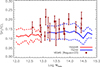 |
Fig. 2. Ratio between the SH-ICL mass as a function of halo mass. The predictions from our model (red and blue lines) are compared to the extrapolated observed data by Ragusa et al. (2023) from the VEGAS survey (brown symbols). Our model aligns reasonably well with the observations, and both indicate no significant relation with halo mass. |
To conclude our analysis, in Figure 3, we present the fraction of stellar mass in the SH relative to the total stellar mass within the virial radius of the halo as a function of halo mass. As with the previous figures, the model predictions are compared with extrapolations from the VEGAS survey data along with the measurements by Deason et al. (2019) for the Milky Way. There is no correlation observed across almost the entire halo mass range probed, although there is a hint of a decreasing fraction at smaller scales predicted by YS50HR, which once the resolution of the simulation is taken into account, should align with YS200. This finding is a direct consequence of the lack of correlation seen in Figure 2 in conjunction with the known relationship between the ICL fraction and halo mass (e.g., Contini et al. 2024c). The VEGAS data show reasonable agreement at low mass scales but tend to be higher for more massive objects. In light of these results, we now proceed to the next section, where we discuss our findings and draw conclusions.
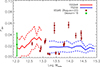 |
Fig. 3. Fraction of SH mass with respect to the total mass within the virial radius of the halo presented as a function of halo mass. Similar to the ICL fraction in the same halo mass range (Contini et al. 2024c), there is no correlation observed in groups and clusters. However, there are indications of a decreasing fraction on smaller scales than loose groups, once the resolution of the simulations is taken into account. Our model predictions (red and blue lines) are compared with the extrapolated observed data by Ragusa et al. (2023) from the VEGAS survey (brown symbols) and the SH mass fraction reported by Deason et al. (2019) for the Milky Way (green symbol). |
4. Discussion and conclusions
The typical radius at which the ICL begins to dominate the light distribution has been investigated both observationally and theoretically by several authors (Iodice et al. 2016; Spavone et al. 2020, 2024; Gonzalez et al. 2021; Montes et al. 2021; Contini et al. 2022; Proctor et al. 2024 and references therein) in recent years. From an observational perspective, the transition radius Rtrans, which we remind the reader represents the point where ICL light predominates in the distribution–that is, where the CG plus ICL light distribution exhibits a clear break–has been found to be approximately 60–80 kpc. These values have also been confirmed by Contini et al. (2022), where Rtrans was defined as the typical radius at which the ICL mass comprises given percentages (> 50%) of the total mass locally. In that study, the authors employed the same assumptions used here to determine the scale radius of the ICL distribution, although the parameter γ in this analysis is better constrained.
Despite the good agreement between observations and theory, Contini et al. (2022) did not formally consider nor define any transition region between the CG and the ICL, in contrast to the present work. Indeed, their definition of Rtrans relies solely on the mass distribution of the CG and ICL. Here, we define Rtrans as the radius that characterizes the SH, which in turn defines the transition region between the CG and ICL. An independent study by Proctor et al. (2024) employed a similar (but not identical) definition of Rtrans to the one used in Contini et al. (2022). While the latter focused on the mass profiles of the CG and ICL, Proctor et al. (2024) considered the density profile. They clearly demonstrated that, due to their definition, Rtrans is an increasing function of halo mass. As shown in Figure 1, this is also true for our predictions, which are more closely linked to the results of Proctor et al. (2024) than to those of Contini et al. (2022) 3 but remain independent of them.
An increasing Rtrans with halo mass is also more physically understandable. Indeed, more massive CGs reside in more massive halos, which also have a larger amount of ICL due to the larger number of galaxies that are subject to stripping or that can merge. From this perspective, it is reasonable to expect a more extended transition region between the two components (i.e., a larger SH). A key point of this Letter is that our new definition of the transition radius not only agrees very well with independent predictions from simulations, but it is also capable of isolating a region where stars do not formally belong to the galaxy’s bulge or disk, nor do they belong to the ICL anymore. We have assumed this region to be the SH that is observed in nearby galaxies and well measured in our own.
To demonstrate the validity of our definition, and thus our assumptions, the predicted SH mass must be comparable to observed values. In Figure 2, we first compared the ratio between the mass in the SH and that of the ICL. Considering the scarcity of SH measurements outside the Local Group (e.g., Beltrand et al. 2024) and given the necessity of resolving the stellar kinematics, we used the same assumptions employed in our model to extrapolate the SH from the VEGAS ICL measurements. These data suggest that the mass in SHs can range between 5% and 20% (including scatter) of that in the ICL, which aligns very well with our model predictions, which range from 7% to 18%.
Similarly, in Figure 3, we showed that our model predicts a fraction of SH mass with respect to the total stellar mass of up to around 5%, indicating that the SH is less significant than both the bulge and disk of the galaxy combined, as well as the ICL. According to recent results by Brown et al. (2024), who investigated the assembly of the ICL in ten groups and clusters extracted from the Horizon-AGN simulation, the SH appears to be the least important component, following satellite galaxies, CGs, and ICL in terms of stellar mass within the virial radius. However, there is no trend with halo mass in either case regarding the ICL mass and the total stellar mass. Considering that the ICL fraction also does not depend on the halo mass at group and cluster scales, this implies that more extended SHs are hosted by more massive halos (Figure 1), but their larger mass is balanced by the greater mass in the ICL and total stellar mass (Figures 2 and 3).
Clearly, our analysis is not without uncertainties related to how we treated the observed data. The information we used to extrapolate our results comes from separating the CG and the ICL, a process that can lead to underestimating or overestimating the ICL depending on the masking applied to nearby satellite galaxies and the method used for the separation. This may account for the larger scatter observed in the VEGAS data.
To conclude, based on the analysis presented in Section 3 and the considerations discussed above, we highlight the key points and conclusions of this Letter:
-
The SH can be associated with the transition region between the galaxy and the ICL, and its radius, Rtrans, can be regarded as the boundary between the CG and the ICL, through the SH.
-
Our new definition of Rtrans aligns well with that used in Proctor et al. (2024). In both cases, the transition radius increases with halo mass (Figure 1), indicating that SHs in clusters are more extensive than those in smaller groups.
-
The fraction of SH mass relative to the ICL and total stellar mass (Figures 2 and 3) is in good agreement with extrapolations from observed data (from the VEGAS survey) and with measurements by Deason et al. (2019) for the SH of our galaxy. Generally, the SH represents only a small fraction of the total stellar mass within the virial radius of the halo, typically around 7% to 18% (model predictions) or 5% to 20% (extrapolated from observed data) of the ICL mass.
The next step in investigating SH formation is to repeat the analysis as a function of redshift and examine potential dependencies on halo formation time and its dynamical state, which is likely considering recent findings such as those by Ragusa et al. (2023), Contini et al. (2023, 2024c), and others for the ICL. Furthermore, we aim to study how properties such as the colors and metallicity of the SH evolve over time and explore their potential connection with those of the ICL.
In this Letter, we use the terms ICL and diffuse light interchangeably.
The gap in halo mass between the two predictions is given by the box of the simulations. In YS50HR, we avoid halos more massive than logMhalo = 13 in order to have enough statistics and halos less massive than logMhalo ∼ 13.2 in YS200 for reasons linked to the resolution.
Here, Rtrans is derived directly from the definition of halo concentration, which depends on the virial radius and the scale radius. The computation of the latter is based on the density profile.
Acknowledgments
The authors thank the anonymous referee for their constructive comments, which have significantly contributed to improving this manuscript. E.C. and S.K.Y. acknowledge support from the Korean National Research Foundation (2020R1A2C3003769), (2022R1A6A1A03053472), and E.C. acknowledges support from the Korean National Research Foundation (RS-2023-00241934). M.S. and E.I. acknowledge the support by the Italian Ministry for 1224 Education University and Research (MIUR) grant PRIN 2022 2022383WFT 1225 “SUNRISE”, CUP C53D23000850006 and by VST funds. R.R. acknowledges financial support through grants PRIN-MIUR 2020SKSTHZ and through INAF-WEAVE StePS founds.
References
- Abadi, M. G., Navarro, J. F., & Steinmetz, M. 2006, MNRAS, 365, 747 [Google Scholar]
- Amorisco, N. C. 2017, MNRAS, 464, 2882 [Google Scholar]
- Arnaboldi, M., & Gerhard, O. 2022, Front. Astron. Space Sci., 9, 403 [NASA ADS] [CrossRef] [Google Scholar]
- Bahé, Y. M., Barnes, D. J., Dalla Vecchia, C., et al. 2017, MNRAS, 470, 4186 [Google Scholar]
- Barnes, D. J., Kay, S. T., Bahé, Y. M., et al. 2017, MNRAS, 471, 1088 [Google Scholar]
- Beltrand, C., Monachesi, A., D’Souza, R., et al. 2024, A&A, 690, A115 [NASA ADS] [CrossRef] [EDP Sciences] [Google Scholar]
- Brown, H. J., Martin, G., Pearce, F. R., et al. 2024, MNRAS, 534, 431 [NASA ADS] [CrossRef] [Google Scholar]
- Bullock, J. S., & Johnston, K. V. 2005, ApJ, 635, 931 [Google Scholar]
- Capaccioli, M., Spavone, M., Grado, A., et al. 2015, A&A, 581, A10 [NASA ADS] [CrossRef] [EDP Sciences] [Google Scholar]
- Chabrier, G. 2003, PASP, 115, 763 [Google Scholar]
- Child, H. L., Habib, S., Heitmann, K., et al. 2018, ApJ, 859, 55 [NASA ADS] [CrossRef] [Google Scholar]
- Contini, E., & Gu, Q. 2020, ApJ, 901, 128 [NASA ADS] [CrossRef] [Google Scholar]
- Contini, E., De Lucia, G., Villalobos, Á., & Borgani, S. 2014, MNRAS, 437, 3787 [Google Scholar]
- Contini, E., Chen, H. Z., & Gu, Q. 2022, ApJ, 928, 99 [NASA ADS] [CrossRef] [Google Scholar]
- Contini, E., Jeon, S., Rhee, J., Han, S., & Yi, S. K. 2023, ApJ, 958, 72 [NASA ADS] [CrossRef] [Google Scholar]
- Contini, E., Yi, S. K., Jeon, S., & Rhee, J. 2024a, ApJS, 274, 41 [NASA ADS] [CrossRef] [Google Scholar]
- Contini, E., Rhee, J., Han, S., Jeon, S., & Yi, S. K. 2024b, AJ, 167, 7 [NASA ADS] [CrossRef] [Google Scholar]
- Contini, E., Han, S., Jeon, S., Rhee, J., & Yi, S. K. 2024c, ApJ, 962, L10 [CrossRef] [Google Scholar]
- Cooper, A. P., Cole, S., Frenk, C. S., et al. 2010, MNRAS, 406, 744 [Google Scholar]
- Cooper, A. P., Parry, O. H., Lowing, B., Cole, S., & Frenk, C. 2015, MNRAS, 454, 3185 [Google Scholar]
- Correa, C. A., Wyithe, J. S. B., Schaye, J., & Duffy, A. R. 2015, MNRAS, 452, 1217 [CrossRef] [Google Scholar]
- Crain, R. A., Schaye, J., Bower, R. G., et al. 2015, MNRAS, 450, 1937 [NASA ADS] [CrossRef] [Google Scholar]
- Deason, A. J., Belokurov, V., Koposov, S. E., & Rockosi, C. M. 2014, ApJ, 787, 30 [NASA ADS] [CrossRef] [Google Scholar]
- Deason, A. J., Belokurov, V., & Sanders, J. L. 2019, MNRAS, 490, 3426 [NASA ADS] [CrossRef] [Google Scholar]
- De Lucia, G., & Helmi, A. 2008, MNRAS, 391, 14 [NASA ADS] [CrossRef] [Google Scholar]
- DeMaio, T., Gonzalez, A. H., Zabludoff, A., et al. 2020, MNRAS, 491, 3751 [Google Scholar]
- D’Souza, R., Kauffman, G., Wang, J., & Vegetti, S. 2014, MNRAS, 443, 1433 [Google Scholar]
- Duc, P.-A., Cuillandre, J.-C., Karabal, E., et al. 2015, MNRAS, 446, 120 [Google Scholar]
- Gonzalez, A. H., George, T., Connor, T., et al. 2021, MNRAS, 507, 963 [NASA ADS] [CrossRef] [Google Scholar]
- Harmsen, B., Monachesi, A., Bell, E. F., et al. 2017, MNRAS, 466, 1491 [Google Scholar]
- Harris, K. A., Debattista, V. P., Governato, F., et al. 2017, MNRAS, 467, 4501 [NASA ADS] [CrossRef] [Google Scholar]
- Hartke, J., Arnaboldi, M., Gerhard, O., et al. 2022, A&A, 663, A12 [NASA ADS] [CrossRef] [EDP Sciences] [Google Scholar]
- Helmi, A. 2008, A&ARv, 15, 145 [CrossRef] [Google Scholar]
- Helmi, A. 2020, ARA&A, 58, 205 [Google Scholar]
- Helmi, A., White, S. D. M., de Zeeuw, P. T., & Zhao, H. 1999, Nature, 402, 53 [Google Scholar]
- Helmi, A., Babusiaux, C., Koppelman, H. H., et al. 2018, Nature, 563, 85 [Google Scholar]
- Ibata, R. A., Lewis, G. F., McConnachie, A. W., et al. 2014, ApJ, 780, 128 [Google Scholar]
- Iodice, E., Capaccioli, M., Grado, A., et al. 2016, ApJ, 820, 42 [Google Scholar]
- Iodice, E., Spavone, M., Capaccioli, M., et al. 2021, The Messenger, 183, 25 [NASA ADS] [Google Scholar]
- Lane, J. M. M., Bovy, J., & Mackereth, J. T. 2022, MNRAS, 510, 5119 [NASA ADS] [CrossRef] [Google Scholar]
- Longobardi, A., Arnaboldi, M., Gerhard, O., & Hanuschik, R. 2015, A&A, 579, A135 [NASA ADS] [CrossRef] [EDP Sciences] [Google Scholar]
- Monachesi, A., Gómez, F. A., Grand, R. J. J., et al. 2019, MNRAS, 485, 2589 [NASA ADS] [CrossRef] [Google Scholar]
- Montes, M., & Trujillo, I. 2019, MNRAS, 482, 2838 [Google Scholar]
- Montes, M., Brough, S., Owers, M. S., & Santucci, G. 2021, ApJ, 910, 45 [Google Scholar]
- Navarro, J. F., Frenk, C. S., & White, S. D. M. 1997, ApJ, 490, 493 [Google Scholar]
- Pillepich, A., Madau, P., & Mayer, L. 2015, ApJ, 799, 184 [Google Scholar]
- Pillepich, A., Nelson, D., Hernquist, L., et al. 2018, MNRAS, 475, 648 [Google Scholar]
- Prada, F., Klypin, A. A., Cuesta, A. J., Betancort-Rijo, J. E., & Primack, J. 2012, MNRAS, 423, 3018 [NASA ADS] [CrossRef] [Google Scholar]
- Proctor, K. L., Lagos, C. d. P., Ludlow, A. D., & Robotham, A. S. G. 2024, MNRAS, 527, 2624 [Google Scholar]
- Ragusa, R., Spavone, M., Iodice, E., et al. 2021, A&A, 651, A39 [NASA ADS] [CrossRef] [EDP Sciences] [Google Scholar]
- Ragusa, R., Mirabile, M., Spavone, M., et al. 2022, Front. Astron. Space Sci., 9, 852810 [CrossRef] [Google Scholar]
- Ragusa, R., Iodice, E., Spavone, M., et al. 2023, A&A, 670, L20 [NASA ADS] [CrossRef] [EDP Sciences] [Google Scholar]
- Schaye, J., Crain, R. A., Bower, R. G., et al. 2015, MNRAS, 446, 521 [Google Scholar]
- Schipani, P., Noethe, L., Arcidiacono, C., et al. 2012, J. Opt. Soc. Am. A, 29, 1359 [Google Scholar]
- Spavone, M., Capaccioli, M., Napolitano, N. R., et al. 2017, A&A, 603, A38 [NASA ADS] [CrossRef] [EDP Sciences] [Google Scholar]
- Spavone, M., Iodice, E., van de Ven, G., et al. 2020, A&A, 639, A14 [NASA ADS] [CrossRef] [EDP Sciences] [Google Scholar]
- Spavone, M., Krajnović, D., Emsellem, E., Iodice, E., & den Brok, M. 2021, A&A, 649, A161 [NASA ADS] [CrossRef] [EDP Sciences] [Google Scholar]
- Spavone, M., Iodice, E., D’Ago, G., et al. 2022, A&A, 663, A135 [NASA ADS] [CrossRef] [EDP Sciences] [Google Scholar]
- Spavone, M., Iodice, E., Lohmann, F. S., et al. 2024, A&A, 689, A306 [NASA ADS] [CrossRef] [EDP Sciences] [Google Scholar]
- Venhola, A., Peletier, R., Laurikainen, E., et al. 2017, A&A, 608, A142 [NASA ADS] [CrossRef] [EDP Sciences] [Google Scholar]
- Wright, A. C., Tumlinson, J., Peeples, M. S., et al. 2024, ApJ, 970, 70 [NASA ADS] [CrossRef] [Google Scholar]
All Figures
|
Fig. 1. Transition radius between the SH and the surrounding ICL as a function of halo mass. Our model predictions (red and blue lines) are compared with the results from Proctor et al. (2024) based on the Eagle (cyan and orange symbols) and C-Eagle (green symbols) simulations and extrapolations of observed data by Ragusa et al. (2023) from the VEGAS survey (brown symbols). For comparison, we show with dashed (YS50HR) and solid (YS200) black lines the scale radius-halo mass relation. Our model predictions are in very good agreement with both theoretical and observational measurements across the entire halo mass range investigated, and all data indicate an increasing transition radius with halo mass. |
| In the text | |
|
Fig. 2. Ratio between the SH-ICL mass as a function of halo mass. The predictions from our model (red and blue lines) are compared to the extrapolated observed data by Ragusa et al. (2023) from the VEGAS survey (brown symbols). Our model aligns reasonably well with the observations, and both indicate no significant relation with halo mass. |
| In the text | |
|
Fig. 3. Fraction of SH mass with respect to the total mass within the virial radius of the halo presented as a function of halo mass. Similar to the ICL fraction in the same halo mass range (Contini et al. 2024c), there is no correlation observed in groups and clusters. However, there are indications of a decreasing fraction on smaller scales than loose groups, once the resolution of the simulations is taken into account. Our model predictions (red and blue lines) are compared with the extrapolated observed data by Ragusa et al. (2023) from the VEGAS survey (brown symbols) and the SH mass fraction reported by Deason et al. (2019) for the Milky Way (green symbol). |
| In the text | |
Current usage metrics show cumulative count of Article Views (full-text article views including HTML views, PDF and ePub downloads, according to the available data) and Abstracts Views on Vision4Press platform.
Data correspond to usage on the plateform after 2015. The current usage metrics is available 48-96 hours after online publication and is updated daily on week days.
Initial download of the metrics may take a while.