| Issue |
A&A
Volume 708, April 2026
|
|
|---|---|---|
| Article Number | A379 | |
| Number of page(s) | 16 | |
| Section | Astrophysical processes | |
| DOI | https://doi.org/10.1051/0004-6361/202557669 | |
| Published online | 28 April 2026 | |
Sagittarius A* near-infrared flare polarization as a probe of space-time
I. Nonrotating exotic compact objects
1
CENTRA, Faculdade de Engenharia, Universidade do Porto, s/n, R. Dr. Roberto Frias, 4200-465, Porto, Portugal
2
CENTRA, Departamento de Física, Instituto Superior Técnico-IST, Universidade de Lisboa-UL, Avenida Rovisco Pais 1, 1049-001, Lisboa, Portugal
3
Institute of Physics, University of Tartu, W. Ostwaldi 1, 50411, Tartu, Estonia
4
Departamento de Física Teórica, Universidad Complutense de Madrid, E-28040, Madrid, Spain
★ Corresponding author: This email address is being protected from spambots. You need JavaScript enabled to view it.
Received:
13
October
2025
Accepted:
26
February
2026
Abstract
Context. The center of our Galaxy hosts Sagittarius A*, which is a supermassive compact object of ∼4.3 × 10⁶ solar masses and is usually associated with a black hole. Nevertheless, black holes possess a central singularity that is considered unphysical, and an event horizon that leads to loss of unitarity in a quantum description of the system. To address these theoretical inconsistencies, alternative models, collectively known as exotic compact objects, have been proposed.
Aims. We investigate the potential detectability of signatures associated with nonrotating exotic compact objects (ECOs) within the dataset of Sgr A* polarized flares as observed through GRAVITY and the upcoming GRAVITY+.
Methods. We examined a total of eight distinct metrics that originate from four different categories of static and spherically symmetric compact objects: black holes, boson stars, fluid spheres, and gravastars. Our approach involved using a toy model that orbits the compact object in the equatorial plane at the Schwarzschild-Keplerian velocity. Using simulated astrometric and polarimetric data with current GRAVITY uncertainties as well as improved flux uncertainties expected for the GRAVITY+ upgrade, we fit the datasets across all metrics we examined. We evaluated the detectability of the metric for each dataset based on the resulting χred2 and Bayesian information criteria-based Bayes factors.
Results. Plunge-through images of ECOs affect polarization and astrometry in a distinguishable way from the spin of a Kerr black hole. With GRAVITY’s current uncertainties, none of the metrics models are discernible. However, when the data are modeled within a compact boson star background, the corresponding best fit is sufficiently superior to the Kerr fit to rule out the latter. We examined the best expected enhanced flux uncertainties and discovered that a fourfold increase in flux sensitivity enables the detection of some of the exotic compact object models we investigated. The signals of the others are too close to each other to be distinguishable. However, with the GRAVITY+ flux uncertainties, when the data are produced using an ECO model, the best-fit ECO model is significantly preferred (with a BIC-based Bayes factor exceeding two) over the best fit in the Kerr metric, such that the latter can be ruled out. Nevertheless, enhancing the astrophysical complexity of the hot-spot model might diminishes these outcomes.
Conclusions. With the improved sensitivity of GRAVITY+, we expect to be able to determine whether Sgr A* is a Kerr black hole or some form of exotic compact object, although we will not be able to identify the specific ECO models that describe Sgr A* best.
Key words: black hole physics / gravitation / gravitational lensing: strong / polarization / radiative transfer / relativistic processes
© The Authors 2026
 Open Access article, published by EDP Sciences, under the terms of the Creative Commons Attribution License (https://creativecommons.org/licenses/by/4.0), which permits unrestricted use, distribution, and reproduction in any medium, provided the original work is properly cited.
This article is published in open access under the Subscribe to Open model. This email address is being protected from spambots. You need JavaScript enabled to view it. to support open access publication.
1. Introduction
The center of our Galaxy hosts Sagittarius A* (Sgr A*), a supermassive compact object of (4.297 ± 0.012)×106 solar masses at a distance of only 8277 ± 9 pc (GRAVITY Collaboration 2022, 2023). It is surrounded by star clusters, for instance, the so-called S-star cluster, in which stars orbit the compact object. The S-star proximity to Sgr A* and their orbital parameters allowed us to test General Relativity for supermassive compact objects, such as the gravitational redshift for star S2 (GRAVITY Collaboration 2018a) or the Schwarzschild precession (GRAVITY Collaboration 2020b). The orbit of these stars was used to constrain the enclosed extended mass within the apocenter of S2 to be ≤3000 M⊙, that is, ≤0.1% of the mass of the supermassive compact object (GRAVITY Collaboration 2022). The S2 orbit was also used to constrain the presence of scalar clouds (Foschi et al. 2023), vector clouds (GRAVITY Collaboration 2024), and a fifth force (GRAVITY Collaboration 2025) around Sgr A*, without any significant evidence of their presence for scalar and vector clouds, and with upper limits for the fifth force. The closest pericenter passage of the stars detected so far is indeed still at a few thousand gravitational radii rg, that is, not in the strongest gravitational regime. The current observational state of the art cannot fully constrain the nature of the supermassive compact object at the center of the Galaxy (De Laurentis et al. 2023; Dai & Stojkovic 2019).
Although the space-time around black holes can effectively describe the observations mentioned above, these space-times present inherent difficulties from mathematical and physical viewpoints. In essence, black hole space-times are characterized by singularities (Penrose 1965, 1969), which indicates potential incompleteness within the theoretical framework. Moreover, an event horizon in black hole physics leads to the so-called black hole information paradox, in which the thermal nature of Hawking radiation implies a potential loss of information. This contradicts the principle of unitary evolution in quantum mechanics, where information must be preserved over time. This tension between general relativity and quantum theory has been widely discussed since Hawking’s seminal work (Hawking 1976). To remedy these challenges, a number of alternative theoretical models, collectively termed exotic compact objects (ECOs), have been proposed (see Cardoso & Pani 2019 for a review). A subset of these ECO models can emulate similar observational predictions, thereby earning the designation of black hole mimickers.
The Event Horizon Telescope (EHT) has provided the first horizon-scale image of Sgr A* (Event Horizon Telescope Collaboration 2022a). This landmark observation opens the door to testing the nature of compact objects in the strong gravity regime. While the image is broadly consistent with the predictions of General Relativity for a Kerr black hole, it does not definitively rule out the existence of ECOs (Event Horizon Telescope Collaboration 2022b; Carballo-Rubio et al. 2022; Vagnozzi et al. 2023; Shaikh 2023; Ayzenberg et al. 2025). Current resolution and modeling uncertainties allow for a range of ECO models, such as boson stars, gravastars, or wormholes, to remain compatible with the EHT data (Olivares-Sánchez et al. 2024).
Since 2001, outbursts of radiation called flares have been detected from Sgr A* in X-rays (Baganoff et al. 2001; Nowak et al. 2012; Neilsen et al. 2013; Barrière et al. 2014; Ponti et al. 2015; Haggard et al. 2019), near-infrared (NIR; Genzel et al. 2003; Ghez et al. 2004; Hornstein et al. 2007; Hora et al. 2014), and radio (Yusef-Zadeh et al. 2006; Bower et al. 2015; Brinkerink et al. 2015). In the past two decades, Sgr A* flares have been the subject of intense observational campaigns and research, although no consensus has yet been reached on their physical origin. Multiple types of models indeed exist for Sgr A* flares, including red noise (Do et al. 2009), a hot spot (Genzel et al. 2003; Broderick & Loeb 2006; Hamaus et al. 2009), an ejected blob (Vincent et al. 2014), star-disk interaction (Nayakshin et al. 2004), disk instability (Tagger & Melia 2006), or magnetic reconnection (Aimar et al. 2023; Lin et al. 2023).
Based on interferometric measurements with the GRAVITY instrument (GRAVITY Collaboration 2017) at the very large telescope interferometer (VLTI), the GRAVITY Collaboration reported the detection of orbital motion for Sgr A* flares (GRAVITY Collaboration 2018b, 2023) at ∼9 gravitational radii (rg) with a low inclination i ∼ 160° compatible with the constraints from the Event Horizon Telescope Collaboration (2024b) results of i ≈ 150°. This detection brought important constraints on the modeling of Sgr A* flares, favoring hot-spot and ejected blob models. However, the physical origin of Sgr A* flares is still under debate.
Flares occur at only a few gravitational radii in the strong-field regime. They are thus an ideal object based on which to study and constrain the space-time and the nature of Sgr A* (Schwarzschild, Kerr, or non-Kerr). Although the effects of spin or ECOs on the flare light curves are too small to be detected or are degenerate with the model parameters, the measure of the astrometry of flares with GRAVITY was thought to be sufficient to detect the non-Kerr metric signature. However, the low inclination and large uncertainties in the astrometric data do not allow for such a detection (Li et al. 2014; Li & Bambi 2014; Liu et al. 2015; Rosa et al. 2023).
The detection of polarization of Sgr A* flares in the near-infrared (NIR) (GRAVITY Collaboration 2018b, 2023) and in radio (Wielgus et al. 2022) brought new observational constraints on the magnetic field configuration. In both wavelengths, the observed polarization properties (QU-loops and angular polarization velocity) are only compatible with a vertical magnetic field. Vincent et al. (2024) showed that the observed loop(s) in the QU-plane is (are) mainly due to special relativity effects of the orbital motion of the emitting region. However, General Relativity, mainly light bending, also affects the observed QU-loop(s), creating an asymmetry relative to the horizontal axis (Vincent et al. 2024). In other words, linear polarization measured with Stokes parameters is sensitive to space-time curvature.
Recently, Rosa et al. (2025), Tamm et al. (2025) studied the imprint on polarimetry of an orbiting hot spot by nonrotating solitonic boson stars, gravastars, and fluid-sphere models. They showed that the key difference in comparison with Schwarzschild relies on the presence and relative contribution from the additional images (second light ring or plunge-through images1), which mostly affect the polarization fraction, but also the electric vector position angle (EVPA).
The primary objective of this paper is to investigate the potential detectability of signatures associated with nonrotating ECOs within the Sgr A* polarized flares dataset, as observed through the GRAVITY instrument. In Sect. 2 we discuss the various ECO metric models that were taken into consideration for this study, while Sect. 3 elaborates on the flare model itself. The methodological framework is delineated in Sect. 4, followed by the presentation of our findings in Sect. 5. We discuss our results in Sect 6 and summarize and conclude in Sect. 7.
2. Metrics of horizonless exotic compact objects
We analyzed three types of static and spherically symmetric exotic compact objects whose optical properties were previously analyzed with GYOTO in the context of infrared flares and radio (EHT) imaging. These are the solitonic boson star, the relativistic perfect-fluid sphere, and the gravitational vacuum star (gravastar). Table 1 summarizes the model parameters. All the selected models have a shadow that mimics the shadow of a black hole, and they are compatible with EHT observations (see Cardoso & Pani 2019 for a review).
Metric model properties.
2.1. Solitonic boson star
Scalar boson stars consist of localized solutions of self-gravitating scalar fields and have been the subject of intense theoretical effort (Kaup 1968; Ruffini & Bonazzola 1969; Colpi et al. 1986; Friedberg et al. 1987; Jetzer 1992; Schunck & Mielke 2003; Liebling & Palenzuela 2012; Macedo et al. 2013; Grandclément 2017; Cunha et al. 2023). They are found as solutions of the Einstein-Klein-Gordon theory, described by the action
![Mathematical equation: $$ \begin{aligned} S=\int \sqrt{-g}\left[\frac{R}{16\pi }-\frac{1}{2}\partial _\mu \phi ^*\partial ^\mu \phi -\frac{1}{2}V\left(|\phi |^2\right)\right]d^4x, \end{aligned} $$](/articles/aa/full_html/2026/04/aa57669-25/aa57669-25-eq1.gif) (1)
(1)
where R is the Ricci scalar, g is the determinant of the metric gμν, ϕ is the complex scalar field, the asterisk denotes complex conjugation, and |ϕ|2 = ϕ*ϕ, and V is the scalar potential. Different boson star models are obtained depending on the form of the potential V. In particular, solitonic boson stars are described by a potential of the form V = μ2|ϕ|2(1−|ϕ|2/α2)2, where μ is a constant that plays the role of the mass of ϕ, and α is a constant free parameter of the model (see Lee 1987; Rosa et al. 2022 for more details). The main interest in solitonic boson stars lies in the fact that they can be compact enough to develop bound-photon orbits while maintaining their stability against radial perturbations.
Due to the complexity of the Einstein-Klein-Gordon system of field equations, no analytical solutions describing boson stars have been obtained. We considered two numerical solutions of solitonic boson stars with different compactness, a model close to the ultracompact regime (boson star 2), and an ultracompact model (boson star 3) described in detail in Rosa et al. (2023). We excluded the diluted model (boson star 1) as the observed Q-U loops for this model are large (Rosa et al. 2025), which is incompatible with the GRAVITY data (GRAVITY Collaboration 2023). Time-integrated images of an orbiting hot spot at low inclination around these two configurations are shown in the left panels of Fig. 1. The boson star 2 model shows a large bright and thick inner ring corresponding to the plunge-through image, while the boson star 3 model shows a pair of light rings and a smaller, but still bright inner ring, again corresponding to the plunge-through image.
 |
Fig. 1. Time-integrated image of a hot spot orbiting the boson star 2 (top left), boson star 3 (bottom left), fluid sphere 2 (top right), and fluid sphere 3 (bottom right) models with an inclination close to face on (i = 20°). Extracted from Rosa et al. (2025) and Tamm et al. (2025). |
2.2. Relativistic fluid sphere
Relativistic fluid spheres are solutions to Einstein’s field equations in the presence of an isotropic perfect fluid (Tolman 1939; Oppenheimer & Snyder 1939; Buchdahl 1959; Iyer et al. 1985). The interior of these solutions is described in the usual spherical coordinates (t, r, θ, ϕ) by the metric
 (2)
(2)
where M and R are constants that represent the mass and surface radius of the star, respectively. The exterior of these solutions is described by the Schwarzschild solution. We restricted our analysis to smooth solutions, that is, the surface of the star R coincides with the radius at which the interior and exterior solutions were matched, and with a constant volumetric energy density. Under these restrictions, these solutions developed a pair of bound-photon orbits whenever R ≤ 3M, with the limiting case R = 3M corresponding to a single degenerate bound-photon orbit, whereas a singularity is present whenever R ≤ 2.25M. More details about this model can be found in Rosa & Piçarra (2020), Tamm & Rosa (2024). Three models were studied in Tamm et al. (2025) with R = 2.25M (fluid sphere 1), R = 2.5M (fluid sphere 2), and R = 3M (fluid sphere 3), but at low inclination (which is likely the case for Sgr A*), the fluid sphere 1 model presents the same observational features as the Schwarzschild model. Thus, we here only considered the fluid sphere 2 and fluid sphere 3 models. Similarly to the boson star case, the right panels of Fig. 1 show the time-integrated images of a hot spot orbiting the fluid sphere 2 (top row) and fluid sphere 3 (bottom row) models at low inclination. Both of them have a pair of light rings and a small inner ring corresponding to the plunge-through image. The inner ring of fluid sphere 2 is smaller than that of the fluid sphere 3 model. Thus, its contribution to the polarization is smaller.
2.3. Gravastar
Similarly to relativistic fluid spheres, gravitational vacuum stars, or gravastars, are solutions of the Einstein field equations in the presence of an isotropic perfect fluid. In the case of gravastars, this fluid is exotic, satisfying an equation of state of the form p = −ρ, where p is the isotropic pressure, and ρ is the energy density (Mazur & Mottola 2004; Visser & Wiltshire 2004; Mottola & Vaulin 2006; Pani et al. 2009; Mazur & Mottola 2015; Danielsson & Giri 2018; Posada & Chirenti 2019; Mazur & Mottola 2023). The interior of gravastars is described by the metric
 (3)
(3)
where α is a parameter controlling the volumetric mass distribution of the star, and  is the mass function. The exterior of the gravastar is described by the Schwarzschild space-time. The parameter α is bounded between 1 and a minimum value αmin that depends on the model, with α = 1 and α = αmin corresponding to solutions with all mass distributed in the volume or on the surface, respectively. Regardless of the mass distribution, these solutions develop a pair of bound-photon orbits whenever the radius R of the surface of the gravastar, where the interior and exterior space-times are matched, satisfies the condition R ≤ 3M, with the limiting case R = 3M corresponding to a single degenerate bound-photon orbit. More details about this model can be found in Rosa et al. (2024). For α ≠ 1, the grr coefficient of the metric is discontinuous, making the parallel transport of the polarization basis inside the ray tracing code GYOTO impossible (more details in Sect. 3.1). We thus fixed α = 1 and selected three configurations: a model with R = 3M (gravastar 1), R = 2.5M (gravastar 2), and R = 2.01M (gravastar 3). Again, we present the time-integrated images of a hot spot orbiting these three configurations at low inclination in Fig. 2. All configurations present a set of light rings and at least one plunge-through image. The size of the inner plunge-through image decreases with an increase in compacticity, with the most compact configuration (gravastar 3) presenting an additional light ring.
 |
Fig. 2. Time-integrated image of a hot spot orbiting the gravastar models with R = 3M (gravastar 1) in the left panel, R = 2.5M (gravastar 2) in the middle panel, and r = 2.01M (gravastar 3) in the right panel. Extracted from Tamm et al. (2025). |
3. Hot-spot model
We considered an analytical orbiting hot-spot model for the flares of Sgr A* in NIR because this model agrees best with the current data. However, we did not choose any specific physical phenomenon at the origin of the flare to avoid a model dependence. The hot spot was assumed to be a uniform sphere of plasma with a radius of 1 rg that emits synchrotron radiation.
As previously demonstrated (Li et al. 2014; Liu et al. 2015; Rosa et al. 2023) and depicted in Fig. 3, the current uncertainties in astrometry, alongside the fact that the flares from Sgr A* are observed nearly face on, prevent the differentiation between various ECO and Schwarzschild models, emphasizing the necessity for polarization measurements.
 |
Fig. 3. Astrometry of an orbiting hot spot in different metric models and simulated astrometric data with current GRAVITY uncertainties. |
3.1. Polarized ray-tracing
We used the public polarized ray-tracing code GYOTO2 (Vincent et al. 2011; Aimar et al. 2024) to compute the images of the hot-spot model for the four Stokes parameters (I, Q, U, and V) that characterize the total received intensity (Stokes I) and the polarization of the received light (Q and U for linear polarization and V for circular polarization). We ignored the circular polarization V as it is not measurable by GRAVITY.
For each observing time, we computed the field-integrated polarized fluxes FI(t), FQ(t), and FU(t) in Jansky, and the centroid position of the total flux (X(t),Y(t)) from the computed images. While polarization strongly depends on the orbital parameters and the inclination (see below), the incorporation of the astrometry allowed us to break some degeneracies. For the remainder of the paper, the field of view was set to 2.6 times the orbital radius in M units to optimize the computation time, and the default resolution was 300 × 300 pixels. This resolution is sufficient to obtain the low-order plunge-through images from the ECO models, but not the high-order images, which require an extreme resolution, but have a minor effect on the observed fluxes. The observed wavelength was set to that of GRAVITY, that is, 2.2 μm.
3.2. Orbital motion
For this theoretical study, we chose the simplest type of orbital motion, that is, a circular orbit at radius r in the equatorial plane. Neither the velocity of the Sgr A* IR flares nor the spin of Sgr A* are well constrained because of the large astrometric uncertainties. Some recent studies suggested a possible super-Keplerian motion (GRAVITY Collaboration 2018b; Aimar et al. 2023; Antonopoulou & Nathanail 2024; Yfantis et al. 2024a,b; Xie et al. 2025). Moreover, as shown in Fig. 3, the astrometric tracks in the ECOs metric are smaller for the same orbital radius because the inner plunge-through images contribute. Thus, when we wished to fit simulated data of a Keplerian orbit in an ECO metric (see more details in Sect. 4) using the Kerr metric, the apparent orbital radius was smaller, and the velocity was sub-Keplerian. In contrast, when we fit simulated data of a Keplerian orbit in Kerr using an ECO metric, the apparent orbit was larger with a super-Keplerian motion. Thus, we allowed the orbital velocity to be a free parameter in the form of the coefficient Kcoef, which is the fraction of the Schwarzschild Keplerian velocity. The orbital motion is thus defined in Boyer-Lindquist coordinates as
 (4)
(4)
with a the spin of the compact object (only for the Kerr metric in this study).
3.3. Electron energy distribution function
The IR flux from Sgr A* flares is thought to be generated by synchrotron radiation from a nonthermal population of electrons (GRAVITY Collaboration 2021). We thus considered a κ distribution of electrons (Marszewski et al. 2021) for our hot spot. This distribution was characterized by a thermal core with a temperature Te and a power-law tail with κ index3 and a number density ne. These three parameters affect the fluxes strongly, while the κ index governs the NIR spectral index. To simplify and limit the number of parameters, we set the number density to 107 cm−3, the temperature to 5 × 10¹⁰ K, and the κ index to 3.5. The overall flux of the generated synthetic flares with these settings matches the usual observed flux from Sgr A* flares (≈10 mJy). Not all flares have the same maximum flux. To mitigate this, we restricted the study to the normalized polarized fluxes Q/I and U/I.
3.4. Magnetic field configuration
The average of the polarization measurements of multiple flares made by GRAVITY shows a single loop of polarization over one orbital period of P = 60 min that constrains the magnetic field configuration to be vertical and the inclination to i = 157° ±5° (see Fig. 4 of GRAVITY Collaboration 2023). This magnetic field configuration was also investigated for ECO-metrics (Rosa et al. 2025; Tamm et al. 2025). We thus restricted our study to this magnetic field configuration. The magnetic field strength is defined through the magnetization parameter σ = B2/4πmpc2ne, which we fixed to 0.01. The magnetic field strength was thus around 43 G, which is the expected order of magnitude for Sgr A* flares (von Fellenberg et al. 2025). In this model, this parameter is only a scaling factor of the total flux.
The observed linear polarization fraction of Sgr A* flares is ∼10 − 40% (GRAVITY Collaboration 2020c), which is much lower than the linear polarization fraction expected from a purely ordered magnetic field (without any stochastic component). A probable explanation is that the magnetic field is only partially ordered, that is, with a stochastic component, as suggested by the EHT observation of Sgr A* (Event Horizon Telescope Collaboration 2024b). This effectively reduces the observed polarization fraction (Rybicki & Lightman 1979). The contribution of plunge-through images can also result in a decrease of the linear polarization fraction, but only for a specific part of the orbit, and it cannot cause the global difference of polarization fraction. To take into account the low observed polarization fraction compared to the models, we applied a constant scaling factor lp to the modeled polarized quantities (Stokes Q and U) from GYOTO, whose value is [0,1]4.
3.5. Parameter summary
Our model had a total of six free parameters. The hot spot had five free parameters, summarized in Table 2: inclination (i), orbital radius (r), initial azimuthal angle (φ0), orbital velocity through the fraction of the Keplerian velocity coefficient (Kcoef), and the polarization factor (lp). The last parameter is the background metric (metric model). We fixed the position angle of the line of nodes to 177.3° following GRAVITY Collaboration (2023) as this parameter adds an unnecessary degree of freedom for this theoretical study.
Parameters of the hot-spot model.
The effect of the spin of a Kerr black hole on the polarization measurements Q/I and U/I could be similar to the effect of the plunge-through images from the ECOs metrics. Thus, to test whether an ECO signature can be fit and thus mimicked by the spin of a Kerr black hole, we added the spin as a free parameter in the Kerr metric (see Sect. 5.2).
4. Method
To determine the detectability of the metrics we considered, we fit simulated data with all aforementioned metrics and compared the results of these fits. Using statistical criteria, we concluded on the detectability of the metrics. The following section describes our method in detail.
4.1. Generation of simulated data
We generated simulated data following the set of parameters presented in Table 2 for the hot spot within a given background metric. In order to accommodate the uncertainties inherent to the observational data, we introduced a random variable to the simulated data points that was drawn from a Gaussian distribution. For the simulated data on astrometric measurements, the Gaussian distribution is characterized by a standard deviation denoted σAstro = 30 μas. For the simulated polarized flux measurements (I, Q and U), the standard deviation we introduced is flux dependent as
 (5)
(5)
with  and I in mJy. The flux dependence of Eq. (5) was reported by GRAVITY Collaboration (2020a) and was calibrated here with the uncertainties from (GRAVITY Collaboration 2023)5. The uncertainties associated with the ratios Q/I and U/I were derived by propagating the measurement errors in I, Q, and U. In Sect. 5 we investigate the detectability of the ECOs with various flux uncertainties in the form of a fraction of Eq. (5), from 1 being the actual GRAVITY uncertainties until
  , which correspond to the best anticipated improved precisions for the GRAVITY+ upgrade (Bourdarot et al. 2024).
The observational duration and data point intervals were by default calibrated to resemble those of GRAVITY, namely, one measurement every 5 minutes, resulting in a total of 12 observations, amounting to 60 minutes overall. This is equivalent to one full orbital period. In Sect. 5 we also investigate the effect of a better time sampling on the detectability of the metrics.
4.2. Fitting
4.2.1. Fitting procedure
In contrast to the five hot-spot parameters, the metric parameter is not continuous (a range of values), but is instead categorical, that is, the choice of a configuration. The treatment of this parameter is thus different from the others. As part of our fit strategy, we opted to individually fit the five (six for Kerr) remaining parameters of our model, namely, the inclination, the orbital radius, the initial azimuthal angle, the orbital velocity scaling factor, and the polarization factor (plus the spin in Kerr), within the context of all possible ECO + Kerr background metrics.
We performed a classical χ2 minimization using the scipy.least_square algorithm with the trust region reflective method. This combination was selected because it is well suited to large bounded optimization problems, which corresponds to our situation, which involves five or even six parameters with clearly defined limits. Another important aspect of the fitting strategy is the computational cost. Each model evaluation requires several minutes, so a single fit typically ranges from about 2 to 12 hours, depending on the chosen metric. This type of algorithm is highly dependent on the initial guess. To reduce the risk of converging to a local minimum, we adopted as our first guess the point with the minimum reduced chi-square, χred2, obtained from a preliminary grid search (see Appendix A for details on the grid). We evaluated the χred2 as
 (6)
(6)
where ν = n − k is the number of degrees of freedom, n being the number of data points and k the number of free parameters, xi the data point i, μi the model, and σi the uncertainty of data point i. We also computed the Bayesian information criterion (BIC) as (Kass & Raftery 1995)
 (7)
(7)
to obtain the statistical criteria of the different fits to be compared to the others.
4.2.2. Evaluate the detectability of a metric
To assess detectability, the primary requirement is that the best-fitting metric, that is, the metric yielding the lowest reduced chi-square, χred2, matches the background metric used to generate the simulated data. The effect of the plunge-through images (induced by the background metric) might not be strong enough to result in a significantly better fit in terms of χred2 for one metric relative to the others, however, or it might mimic the effect of the spin of a Kerr black hole (or vice versa) and thus lead to comparable χred2 values. For this reason, we additionally employed the BIC-based Bayes factor K between the best-fitting metric and the second-best-fitting metric, that is, the metric with the second-lowest χred2. The BIC-based Bayes factor was evaluated following Wagenmakers (2007) as
![Mathematical equation: $$ \begin{aligned} \log _{10}\,\mathrm{K} = \log _{10} \left[ \exp \left(\frac{\Delta \mathrm{BIC}}{2} \right) \right], \end{aligned} $$](/articles/aa/full_html/2026/04/aa57669-25/aa57669-25-eq11.gif) (8)
(8)
with ΔBIC the difference of BIC between the second-best-fitting and best-fitting metrics.
For each background metric and uncertainty levels, we generated ten simulated datasets. Even limited, this number of simulated datasets allowed us to deriving statistics (average and standard deviation) on the lowest χred2, the associated BIC, and more importantly, on log10 K with limited computational cost. We thus defined four detectability outcomes according to the value of log10 K and following the Kass & Raftery (1995) scale. We list them below.
-
Risk of mismatch: The best-fitting metric does not always correspond to the background metric in the simulated data, meaning that there is a risk of mismatch of metrics (symbolized by ✗✗).
-
Not detectable: log10 K < 1. The best-fitting metric corresponds to the background metric in the simulated data, but the second-best-fitting metric is equivalent to the best-fitting metric (symbolized by ✗).
-
Partially detectable: 1 ≤ log10 K ≤ 2. In this case, the best-fitting metric is significantly better, but not enough to make a strong statement (symbolized by [∼]).
-
Detectable: log10 K > 2. The best-fitting metric is considerably better than the second-best-fitting metric and is thus detectable (symbolized by ✓).
A sketch summarizing the whole procedure is shown in Fig. 4.
 |
Fig. 4. Sketch illustrating our method for assessing the detectability of ECO models. |
Although some ECO metrics are difficult to distinguish from one another, it is also interesting to examine whether, even when it is not detectable, a metric can be distinguished from the Kerr solution. To this end, we calculated the BIC-based Bayes factor between the best-fitting metric and Kerr, denoted as log10 K|Kerr. We adopted the same notation as used for the detectability analysis when we assessed the exclusion of the Kerr metric.
5. Results
5.1. Current GRAVITY uncertainties
We first tested the detectability of the studied ECO metrics with current GRAVITY uncertainties. We generated ten simulated data with σAstro = 30 μas and the σFlux from Eq. (5) in all previously listed background metrics. For each of the generated datasets, we performed a fit in all background metrics, whose results are listed in Table 3. This table shows for each simulated data we generated in a given background metric (each line) the average best reduced chi-squared ⟨χred2⟩ with its standard deviation (second column), the average associated BIC with its standard deviation (third column), and the average and standard deviation of the logarithmic BIC-based Bayes factor ⟨log10 K⟩ (forth column). Columns 5 and 6 highlight the detectability of the metric used to generate the simulated data compared to all other metrics and compared to Kerr alone, or according to the criteria listed in Sect. 4.2.2. Column 6 also reports the average BIC-based Bayes factor between the best-fitting metric and Kerr, with its standard deviation.
Fit summary results for the metrics and Bayesian criteria with GRAVITY uncertainties.
The first main conclusion from Table 3 is that none of the metric signatures can be clearly detected from the other with GRAVITY uncertainties (⟨log10 K⟩ is always below 1). This is an expected result because so far, all tests we made are compatible with the Kerr solution. Moreover, in all cases, there is a risk of mismatch between the background and the best-fitting metric. For most metrics, with the exception of boson star 2, of the ten simulated datasets generated from a given background metric, none of the fitted metrics clearly outperformed another, and no clear trend emerges. In other words, at this level of flux uncertainty, no mismatch occurs between a particular pair of metrics, but it rather affects all candidate metrics. This arises because the effect of the metric (e.g., spin in the Kerr case, or plunge-through images for ECOs) on the astrometric and polarimetric observables is not strong enough relative to the uncertainties to break the degeneracies with the hot-spot parameters. Slightly different hot-spot parameters in two distinct metrics can thus produce observables that agree within the error bars.
However, as noted previously, this behavior is not seen for the boson star 2 model. Of the ten simulated datasets, boson star 2 is not the best-fitting metric in only one case. The data are better fit there by the gravastar 1 metric, with χred2 = 1.22 and ⟨log10 K⟩ = 0.05. In this dataset, the fit quality for gravastar 1 and boson star 2 is therefore essentially the same. In all other cases, we clearly recovered the boson star 2 metric. This behavior arises from the large angular size and relative brightness of the plunge-through images in this model (see the top left panel of Fig. 1), which strongly affect the observed polarization fraction and EVPA (Rosa et al. 2025). This is illustrated in Fig. 5, which shows the contributions of the different image orders and types. The contribution of the plunge-through images varies with time and orbital phase. This signal is strong enough that it cannot be mimicked by the spin of a Kerr black hole, as indicated by the BIC-based Bayes factor between the boson star and Kerr fits of ⟨log10 K|Kerr⟩ = 3.9 ± 1.6. Thus, even with GRAVITY uncertainties, if Sgr A* is a boson star (boson star 2 model), the data should still be better described by this model than by Kerr. This is illustrated in Fig. 6, which shows the fits to one simulated dataset with a boson star 2 background, using both the boson star 2 and Kerr metrics. The fit values are summarized in Table 4.
 |
Fig. 5. Contribution of the various image orders and nature, i.e., primary only as dotted lines, primary + secondary (equivalent to Schwarzschild) as dashed lines, and all images including the plunge-through images as solid lines. |
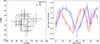 |
Fig. 6. Simulated data, generated in the boson star 2 metric and represented by dots with error bars (reflecting GRAVITY-like uncertainties), compared with two best-fit models: one model in the boson star 2 metric (solid line), and the other in the Kerr metric (dashed lines). Left: astrometry. Right: time evolution of Q/I in red and U/I in blue. |
Results of fitting one of the simulated data generated in the boson star 2 metric (with GRAVITY uncertainties) for the best-fitting metric (the boson star 2 model) and Kerr.
5.2. Spin versus ECO signatures
A central point of our analysis is the possibility that the polarization arising from plunge-through images in the horizonless ECO metric models we studied can mimic the effects of the spin of a Kerr black hole (and vice versa). In Fig. 7 we present the normalized polarization fluxes Q/I(t) and U/I(t) over one orbit, using the hot-spot parameters from Table 2, for various metrics, including ECOs and Kerr space-times with spins a = −0.9 (orange) and a = 0.9 (green). The signal amplitudes relative to the Schwarzschild case (solid black curves) are broadly comparable between the spinning black holes and the ECO models (with the exception of the boson star 2 model, as noted previously). However, the time dependence of the polarization differs across the various metrics, which in principle allows them to be distinguished observationally.
 |
Fig. 7. Normalized polarized fluxes of a hot spot orbiting various compact metric models: Schwarzschild as full black lines, the boson star 2 model as dashed lines, the fluid sphere 2 model as dotted lines, the gravastar 2 model as dash-dotted lines, and two Kerr metrics with spin value of a = −0.9 in orange and a = 0.9 in green. The parameters for the hot spot are listed in Table 2. |
5.2.1. Fitting an ECO with Kerr
In this section, we examine the effect of the fitting procedure on a simulated dataset generated in an ECO model with the Kerr metric. Due to the contribution of plunge-through images, the astrometric signal is shrunk compared to the Schwarzschild case. Consequently, when fitting simulated data (astrometry + polarimetry) generated in an ECO model with the Kerr metric, the inferred orbital radius is generally expected to be smaller than the true input radius. This trend is observed in most cases, but the large astrometric uncertainties prevent us from placing tight constraints on this parameter.
In addition, the orbital velocity scaling factor Kcoef is affected by the value of the orbital radius, and it thus separates the spatial from the temporal characteristics of the flares. Because astrometric data provide only weak spatial constraints whereas polarimetric observations impose strong temporal constraints, changes in the orbital radius translate directly into changes in the inferred Kcoef. Consequently, the two parameters are strongly correlated, as illustrated by the corner plot in Fig. 8.
 |
Fig. 8. Corner plot illustrating the parameter fit for a single simulated dataset, generated and fit in the boson star 2 metric (corresponding to Table 4 and to the full line of Fig. 6). |
We observed that when simulated data generated in an ECO model were fit using a Kerr metric, the inferred linear polarization factor was significantly reduced relative to its true input value. Consequently, a low measured polarization fraction might falsely suggest the presence of plunge-through images. Nonetheless, many other poorly constrained astrophysical processes can also modify the polarization fraction. This introduces a complete degeneracy between an ECO-related origin and conventional astrophysical effects, and we therefore do not consider this behavior to be a reliable signature for identifying ECOs.
Finally, as discussed in Sect. 3.5, when fitting any simulated data in the Kerr metric, the black hole spin is treated as a free parameter. We thus allowed the algorithm to exploit this additional degree of freedom when fitting signals that included plunge-through images produced by ECOs. Nevertheless, in ∼83% of the cases (58 out of 70) with GRAVITY-level uncertainties, the best-fit spin for data generated in an ECO metric is statistically consistent with zero. This behavior is illustrated by the fits reported in Table 4. This indicates that varying the spin alone cannot fully reproduce the effects induced by plunge-through images.
Consequently, we examined whether the datasets were best fit by an ECO or Kerr and whether we can exclude the latter. We employed the same statistical diagnostic as in Sect. 4, namely the BIC-based Bayes factor comparing the best-fitting metric to Kerr (⟨log10 K|Kerr⟩). As previously mentioned, for the boson star 2 metric, the corresponding model is statistically preferred over Kerr, but this does not hold for the other metrics when GRAVITY-like uncertainties are assumed. The gravastar 1 and gravastar 2 metrics yield a BIC-based Bayes factor with respect to Kerr (log10 K|Kerr) exceeding one, but still below the threshold (when the uncertainties are taken into account) required to draw a strong conclusion.
5.2.2. Fitting Schwarzschild with an ECO versus with Kerr
We investigated the opposite configuration, namely fitting the simulated dataset in Schwarzschild using an ECO model and a Kerr model (see the first row of Table 3).
First, for five of our ten simulated datasets with GRAVITY uncertainties and based on χred2, we recovered the correct background metric, but for the other five, we found a mismatch. When we retrieved the black hole metric, the BIC value was higher than that of the second best-fitting metric because an additional degree of freedom is allowed in Kerr, that is, the spin. This resulted in a negative ΔBIC, and consequently, in a negative log10 K, explaining the negative value of ⟨log10 K⟩. This means that even if the best-fitting metric is Kerr according to the χred2, this is only due to the spin being free and that this fitting is not significantly better (and is even equivalent) to the fits in ECO models.
Another interesting result is the BIC-based Bayes factor relative to Kerr (⟨log10 K|Kerr⟩). This value is compatible with zero, but has significant error bars. There is even an extreme case for which the simulated data are best fit in the fluid sphere 2 model and have log10 K|Kerr = 2.01, which, in case of a real flare, might account for a detection of the later metric. This highlights the fact that with these uncertainties, there is a risk of false detection. The results of this fit and the comparison with the best-fit in Kerr are shown in Appendix B.
5.3. Improving the detectability of the ECOs
In 2026, the upgrade of the GRAVITY instrument called GRAVITY+ is expected to enter service. This upgrade of the instrument itself also comes with an improvement of the VLTI infrastructure, including a better adaptive optics (AO) system with laser-guide stars on all unit telescopes (UT; 8-meter telescopes) and better fringe-tracking capabilities. The anticipated outcome of these enhancements optimally is an improvement of a factor of ∼7 in the signal-to-noise ratio with respect to flux uncertainties (Bourdarot et al. 2024).
We then investigated how the detectability of the studied ECO models can be improved in the context of the upcoming GRAVITY+ upgrade. The first obvious possibility is to reduce the uncertainties. While smaller flux uncertainties are achievable, it is challenging to reduce the astrometric uncertainties because GRAVITY is currently at the highest astrometric precision. We thus focused on improving the flux sensitivity and investigated two scenarios: 1) smaller flux uncertainties with the same temporal resolution (Sect. 5.3.1), and 2) similar flux uncertainties with a higher temporal resolution (Sect.5.3.2).
5.3.1. Smaller flux uncertainties
We therefore investigated the best improvement on flux uncertainties expected with the GRAVITY+ upgrade. We performed the same analysis as in Sect. 5.1 with an uncertainty of the flux σFlux smaller by seven times.
At the high level of photometric precision achieved, the effect of the plunge-through images, as induced by the various ECO models, exceeds the corresponding uncertainty. As a result, the data are fit significantly better when the same metric is used as was adopted to generate the simulated data, compared with alternative metrics (see Table 5). This effect is especially pronounced for the Schwarzschild, boson star 2 and fluid sphere 2 metrics, all of which satisfy the detectability conditions (zero mismatch and ⟨log10 K⟩ greater than 2). The boson star 3 model also shows enhanced detectability, but its mean BIC-based Bayes factor minus one standard deviation remains below the threshold value of two that is needed to assert detectability.
Results of fitting one of the simulated data generated in the fluid sphere 3 with GRAVITY+ uncertainties for the best-fitting metric (the gravastar 2 model) and in the fluid sphere 3 model.
The remaining metrics, namely fluid sphere 3 and the three gravastar configurations, continue to exhibit mismatches even under these small uncertainties. In the case of fluid sphere 3, only two realizations show a mismatch, specifically, those with the boson star 3 and gravastar 2 models. However, gravastar 2 is most frequently identified as the second-best fit. We further observe that when the simulated datasets are generated in the gravastar 2 background, the most common mismatches occur with the fluid sphere 3 model. This indicates that from an observational standpoint, the signals produced by fluid sphere 3 and gravastar 2 are very similar and remain close enough to each other to induce confusion between the two, even at such low uncertainty levels. In Fig. 9 we present the best-fitting models for these two metrics (fluid sphere 3 shown as solid lines and gravastar 2 as dashed lines) for a single simulated dataset generated in the fluid sphere 3 metric that leads to a mismatch. This figure clearly shows that two metrics can have the same observational properties, with tiny differences leading to a mismatch. For the gravastar 1 configuration, there are once more only two mismatches with the gravastar 2 and boson star 3 models. As in the case of the fluid sphere 3 model, gravastar 2 again emerges as the metric that most frequently provides the second-best fit. This is expected given that the time-integrated images of the gravastar 2 and 3 models shown in Fig. 2 are similar. To enhance the accuracy and detectability of these models, incorporating the radius of the gravastar as a free continuous parameter in the fitting process (an approach that exceeds the boundaries of this paper) instead of selecting discrete values might prove beneficial.
 |
Fig. 9. Same as Fig. 6, but with simulated data in the fluid sphere 3 background and best GRAVITY+ uncertainties. The best-fitting models shown are in the gravastar 2 metric (full lines) and in the fluid sphere 3 metric (dashed lines). |
The case of the gravastar 3 is different from the others. Even with the low uncertainties, there is a significant amount of mismatch (40%) with the fluid sphere 2 models. When we recovered the correct background metric, the second best-fitting metric was always the fluid sphere 2 model, suggesting similar observational properties. However, for the opposite, that is, when the simulated datasets were in fluid sphere 2, this trend of degeneracies was not observed. We show in Fig. 10 one simulated dataset generated in the gravastar 3 model with the best-fit made in the latter metric as full lines and in the fluid sphere 2 model as dashed lines. The associated best-fitted parameters are listed in Table 7. The two signals are very similar and indistinguishable at early times, but they start to differ at later times between t = 35 min and t = 55 min, corresponding to φ ∼ 225° and φ ∼ 345°, respectively. In this region, the primary image is dimmed because of the small pitch angle between the photon wave vector and the ambient vertical magnetic field (lower synchrotron emission). As a consequence, the signals are dominated by the secondary and plunge-through images, which explains the higher difference between the two models.
 |
Fig. 10. Same as Fig. 6, but with simulated data in the gravastar 3 background and best GRAVITY+ uncertainties. The best-fitting models shown are in the gravastar 3 metric (full lines) and in the fluid sphere 2 metric (dashed lines). |
Results of fitting one of the simulated data generated in the gravastar 3 with GRAVITY+ uncertainties for the best-fitting metric (the gravastar 3 model) and in the fluid sphere 2 model.
The most important result is that with the best GRAVITY+ improvement on the flux uncertainties, for all simulated datasets in an ECO metric, the mean BIC-based Bayes factor with Kerr (⟨log10 K|Kerr⟩) minus one standard deviation is higher than two. This means that if the background metric is one of the studied ECOs, we can exclude the Kerr metric even when we cannot fully constrain the nature of the ECO (this depends on the model). We thus will be able to test the Kerr hypothesis using Sgr A*’s flare polarization and astrometry.
We note that these high polarimetric measurements are also achievable by the radio interferometer Atacama Large Millimeter/submillimeter Array (ALMA). However, the environmental effects by the surrounding plasma at radio wavelengths are stronger than in the IR, and there is no possible astrometry because of the angular resolution.
5.3.2. Better time resolution
An alternative utilization of the GRAVITY+ and VLTI enhancements involves reducing the integration time from the standard 5-minute intervals to a more frequent 1-minute interval, while maintaining flux uncertainties comparable to those observed with the GRAVITY measurements. For observation of flares at the Galactic center, such a scenario is more likely than the improvement of a factor of 7 on the flux uncertainties.
The effect of plunge-through images on polarization is not constant over time, as shown by Figs. 5 and 7, suggesting that enhanced temporal resolution, achieved without compromising flux uncertainty, might be enough to effectively differentiate between different metrics. To evaluate this hypothesis, we created simulated datasets in which we captured one data point every minute and repeated the prior procedures to examine the results. However, the fit results for each dataset were broadly consistent with those obtained using the 5-minute cadence, with most values of ⟨log10 K⟩ (again with the exception of BS2) remaining below the threshold of unity. This occurs because although the metric signature is time dependent, the substantial flux uncertainties prevent us from clearly distinguishing the metric signal from the astrophysical parameters. Consequently, this method yields no definitive conclusion, and the most effective strategy is instead to reduce the flux uncertainties.
6. Limitations and discussion
6.1. Limitations
We adopted a simplified hot-spot model characterized by uniform spatial parameters positioned along a circular orbit within the equatorial plane at the Schwarzschild-Keplerian velocity. This model is likely too rudimentary to adequately capture the flares of Sgr A* in NIR observations. The nature of motion, whether circular, helical, or conical, significantly affects the observed astrometry Antonopoulou & Nathanail (2024) and the light curves (Aimar et al. 2023). The electron energy distribution (EED) was presumed to follow a Kappa distribution, with a constant power-law index at high energies, number density, and temperature, while variability is highly expected for flares. Acceleration mechanisms such as magnetic reconnection, for example, and synchrotron cooling play a crucial role in high-energy electrons, and therefore, in flare modeling. With a more sophisticated model that includes more astrophysics (with its uncertainties), it is probable that the detectability of the metrics will decrease as the space-time characteristics might be diluted and degenerated with the astrophysical parameters. This highlights the importance of an accurate flare modeling.
Moreover, we did not account for the quiescent state of Sgr A* so far. Although its effect is low when the flux from the flare is high, the quiescence cannot be neglected when the flux from the flare and the quiescence are comparable, that is, at a later time.
6.2. Discussion
The encouraging results outlined in the previous discussion hold significant implications for the future observations planned with the advanced GRAVITY+ instrument and the upgraded Very Large Telescope Interferometer (VLTI). These advancements aim to detect the elusive ECO signatures in the flares emitted by Sagittarius A* (Sgr A*). Additionally, analogous polarization studies of Sgr A* flares have been conducted at radio frequencies, as detailed by Wielgus et al. (2022). At these wavelengths, considerations such as Faraday rotation and conversion effects cannot be disregarded, as the phenomena of accretion and ejection remain intensely luminous even during flare events. This scenario adds further complexity to the astrophysical processes observed in comparison to those in the NIR spectrum. Despite these challenges, the exceptional temporal resolution provided by ALMA coupled with its remarkable ability to ascertain very low levels of polarized flux uncertainties, renders this instrument an exceedingly promising candidate for the rigorous search for ECO signatures within the radio flares of Sgr A*.
The latest polarized images presented by Event Horizon Telescope Collaboration (2024a) provide a persuasive and distinct opportunity to explore the signatures of ECOs and to examine alternative gravitational theories (Yan 2025; Ahmed & Bouzenada 2024; Aliyan & Nozari 2024; Walia 2024; Vertogradov et al. 2025; Perrucci et al. 2025; Gan et al. 2024; Vishvakarma et al. 2025; Li et al. 2026).
Ultimately, with the improvements brought by the GRAVITY+ upgrade and the enhancements of the VLTI, alongside the anticipated new generation of NIR instruments integrated with the Extremely Large Telescope (ELT), it is anticipated that an increased number of stars will be discerned (Bourdarot et al. 2024), with some being in close proximity to Sgr A*. This advance in observational capability will enable us to conduct further rigorous assessments of general relativity, examine ECO imprints on the trajectories of stellar bodies, and evaluate alternative gravitational theories. Such tests remain independent of the constraints posed by Sgr A* polarized flares and offer a complementary approach.
7. Summary and conclusions
We conducted an in-depth investigation of the detectability of space-time signatures through polarization measurements of individual flares from Sgr A*. For our analysis, we employed an analytical model of a hot spot orbiting the compact object in its equatorial plane, specifically, at the Schwarzschild-Keplerian velocity. Our examination encompassed a comprehensive set of eight different background metrics, derived from four distinct families of compact objects: Schwarzschild black holes, boson stars, fluid spheres, and gravastars. These models included parameters for exotic compact objects crafted to mimic the behavior of regular black holes.
The principal distinction between the ECOs we analyzed and regular black holes are the plunge-through images, whose polarization properties are comparable to the secondary image associated with the black hole space-time. These plunge-through images also contribute to an increased total intensity, which alone is completely degenerate with astrophysical parameters such as the number density or temperature of the hot spot, thereby affecting the observed EVPA and the polarization fraction. To break degeneracies and limit the number of the hot-spot parameters, it becomes imperative to examine the normalized polarized quantities Q/I and U/I and not the original parameters I, Q and U.
To evaluate the detectability of a specified metric, we generated ten simulated datasets in this metric and executed eight fits (one for each metric under investigation) for each of them. The metric with the lowest χred2 value was considered to be the best-fitting metric. To state whether a metric was detectable, we first verified that the best-fitting metric corresponded to the metric we used to generate the simulated data (no mismatch). We then compared the mean BIC-based Bayes factor ⟨log10 K⟩ between the best-fitting metric and the other metrics. If the latter minus one standard deviation was greater than 2, we considered that the best fits were sufficiently better than the others to state that the metric is detectable; otherwise, it was not. We also compared the best-fitting metric to the best-fit in the Kerr metric using the same threshold. This enabled us to determine whether the data favored ECO models over Kerr metrics, or equivalently, whether the Kerr metric was ruled out by the data.
The imprints on polarization measurements from the plunge-through images are, at best, of the same order as the current measurement uncertainties associated with the GRAVITY instrument. As a result, no metric is currently detectable (see Table 3). Nevertheless, for the boson star 2 model, the best-fitting metric (most of the time, the boson star 2 model itself) is statistically significantly better than Kerr to exclude the latter. We also predicted the detectability of ECOs with the upcoming upgrade of the GRAVITY instrument GRAVITY+. With flux uncertainties smaller by about seven times than we can expect with this upgrade, some ECO metrics (the boson star 2 and the fluid sphere 2 models) become detectable, and the boson star 3 model becomes potentially detectable with a limited BIC-based Bayes factor of 3.0 ± 1.4. We examined whether an ECO model can mimic the spin signature of a Kerr black hole, and conversely, whether a Kerr black hole can mimic an ECO. Although the signal amplitudes are broadly similar, their temporal characteristics differ, allowing the two scenarios to be distinguished provided the flux uncertainties are sufficiently good. With the best expected GRAVITY+ performance estimates and for all ECO metrics we considered, the average BIC-based Bayes factor with respect to Kerr (⟨log10 K|Kerr⟩) exceeds the adopted threshold. Consequently, at this level of precision, if Sgr A* were described by one of the ECO models we analyzed, the application of this method would statistically prefer the ECO description over the Kerr solution.
However, the model we used is very simplistic, with very little astrophysics (only the vertical magnetic field configuration from GRAVITY Collaboration (2023) and synchrotron emission). Most of the photometric properties are governed by relativistic effects such as beaming, Doppler boosting, and light bending. In reality, flares are much more complex, with many astrophysical uncertainties that mitigate detectability and might lead to an incorrect best-fit metric. Nevertheless, this advancement opens up a realm of exciting opportunities and holds substantial promise for the future of astronomical observations, paving the way for innovative discoveries and pushing the boundaries of our understanding of the Universe.
Acknowledgments
N.A. and P.G. thanks the Fundação para a Ciência e Tecnologia (FCT), Portugal, for the financial support to the Center for Astrophysics and Gravitation (CENTRA/IST/ULisboa) through grant No. UID/99/2025. The authors thankfully acknowledge the computer resources, technical expertise and assistance provided by CENTRA/IST. Computations were performed at the cluster “Baltasar-Sete-Sóis” and supported by the H2020 ERC Consolidator Grant “Matter and strong field gravity: New frontiers in Einstein’s theory” grant agreement no. MaGRaTh-646597. J. L. R. is supported by the Project PID2022-138607NBI00, funded by MICIU/AEI/10.13039/501100011033 (“ERDF A way of making Europe" and “PGC Generación de Conocimiento”) The authors thank Saurabh, Thibaut Paumard and Frédéric Vincent for fruitful discussions.
References
- Ahmed, F., & Bouzenada, A. 2024, Eur. Phys. J. C, 84, 1271 [Google Scholar]
- Aimar, N., Dmytriiev, A., Vincent, F. H., et al. 2023, A&A, 672, A62 [NASA ADS] [CrossRef] [EDP Sciences] [Google Scholar]
- Aimar, N., Paumard, T., Vincent, F. H., Gourgoulhon, E., & Perrin, G. 2024, Class. Quant. Grav., 41, 095010 [Google Scholar]
- Aliyan, F., & Nozari, K. 2024, Phys. Dark Univ., 46, 101611 [Google Scholar]
- Antonopoulou, E., & Nathanail, A. 2024, A&A, 690, A240 [NASA ADS] [CrossRef] [EDP Sciences] [Google Scholar]
- Ayzenberg, D., Blackburn, L., Brito, R., et al. 2025, Liv. Rev. Relat., 28, 4 [Google Scholar]
- Baganoff, F. K., Bautz, M. W., Brandt, W. N., et al. 2001, Nature, 413, 45 [Google Scholar]
- Barrière, N. M., Tomsick, J. A., Baganoff, F. K., et al. 2014, ApJ, 786, 46 [CrossRef] [Google Scholar]
- Bourdarot, G., & Eisenhauer, F. 2024, in SF2A-2024: Proceedings of the Annual meeting of the French Society of Astronomy and Astrophysics, eds. M. Béthermin, K. Baillié, N. Lagarde, et al., 183 [Google Scholar]
- Bower, G. C., Markoff, S., Dexter, J., et al. 2015, ApJ, 802, 69 [Google Scholar]
- Brinkerink, C. D., Falcke, H., Law, C. J., et al. 2015, A&A, 576, A41 [NASA ADS] [CrossRef] [EDP Sciences] [Google Scholar]
- Broderick, A. E., & Loeb, A. 2006, MNRAS, 367, 905 [Google Scholar]
- Buchdahl, H. A. 1959, Phys. Rev., 116, 1027 [NASA ADS] [CrossRef] [Google Scholar]
- Carballo-Rubio, R., Di Filippo, F., Liberati, S., & Visser, M. 2022, JCAP, 2022, 055 [CrossRef] [Google Scholar]
- Cardoso, V., & Pani, P. 2019, Liv. Rev. Relat., 22, 4 [NASA ADS] [CrossRef] [Google Scholar]
- Colpi, M., Shapiro, S. L., & Wasserman, I. 1986, Phys. Rev. Lett., 57, 2485 [Google Scholar]
- Cunha, P. V. P., Herdeiro, C., Radu, E., & Sanchis-Gual, N. 2023, Phys. Rev. Lett., 130, 061401 [Google Scholar]
- Dai, D.-C., & Stojkovic, D. 2019, Phys. Rev. D, 100, 083513 [Google Scholar]
- Danielsson, U. H., & Giri, S. 2018, J. High Energy Phys., 2018, 70 [Google Scholar]
- De Laurentis, M., de Martino, I., & Della Monica, R. 2023, Rep. Progr. Phys., 86, 104901 [CrossRef] [Google Scholar]
- Do, T., Ghez, A. M., Morris, M. R., et al. 2009, ApJ, 691, 1021 [NASA ADS] [CrossRef] [Google Scholar]
- Event Horizon Telescope Collaboration (Akiyama, K., et al.) 2022a, ApJ, 930, L12 [NASA ADS] [CrossRef] [Google Scholar]
- Event Horizon Telescope Collaboration (Akiyama, K., et al.) 2022b, ApJ, 930, L17 [NASA ADS] [CrossRef] [Google Scholar]
- Event Horizon Telescope Collaboration (Akiyama, K., et al.) 2024a, ApJ, 964, L25 [NASA ADS] [CrossRef] [Google Scholar]
- Event Horizon Telescope Collaboration (Akiyama, K., et al.) 2024b, ApJ, 964, L26 [CrossRef] [Google Scholar]
- Foschi, A., Abuter, R., Aimar, N., et al. 2023, MNRAS, 524, 1075 [Google Scholar]
- Friedberg, R., Lee, T. D., & Pang, Y. 1987, Phys. Rev. D, 35, 3658 [Google Scholar]
- Gan, X., Wang, L.-T., & Xiao, H. 2024, Phys. Rev. D, 110, 063039 [Google Scholar]
- Genzel, R., Schödel, R., Ott, T., et al. 2003, Nature, 425, 934 [NASA ADS] [CrossRef] [Google Scholar]
- Ghez, A. M., Wright, S. A., Matthews, K., et al. 2004, ApJ, 601, L159 [CrossRef] [Google Scholar]
- Grandclément, P. 2017, Phys. Rev. D, 95, 084011 [Google Scholar]
- GRAVITY Collaboration (Abuter, R., et al.) 2017, A&A, 602, A94 [NASA ADS] [CrossRef] [EDP Sciences] [Google Scholar]
- GRAVITY Collaboration (Abuter, R., et al.) 2018a, A&A, 615, L15 [NASA ADS] [CrossRef] [EDP Sciences] [Google Scholar]
- GRAVITY Collaboration (Abuter, R., et al.) 2018b, A&A, 618, L10 [NASA ADS] [CrossRef] [EDP Sciences] [Google Scholar]
- GRAVITY Collaboration (Abuter, R., et al.) 2020a, A&A, 638, A2 [NASA ADS] [CrossRef] [EDP Sciences] [Google Scholar]
- GRAVITY Collaboration (Abuter, R., et al.) 2020b, A&A, 636, L5 [NASA ADS] [CrossRef] [EDP Sciences] [Google Scholar]
- GRAVITY Collaboration (Jiménez-Rosales, A., et al.) 2020c, A&A, 643, A56 [CrossRef] [EDP Sciences] [Google Scholar]
- GRAVITY Collaboration (Abuter, R., et al.) 2021, A&A, 654, A22 [NASA ADS] [CrossRef] [EDP Sciences] [Google Scholar]
- GRAVITY Collaboration (Abuter, R., et al.) 2022, A&A, 657, L12 [NASA ADS] [CrossRef] [Google Scholar]
- GRAVITY Collaboration (Abuter, R., et al.) 2023, A&A, 677, L10 [NASA ADS] [CrossRef] [EDP Sciences] [Google Scholar]
- GRAVITY Collaboration (Foschi, A., et al.) 2024, MNRAS, 530, 3740 [Google Scholar]
- GRAVITY Collaboration (Abd El Dayem, K., et al.) 2025, A&A, 698, L15 [Google Scholar]
- Haggard, D., Nynka, M., Mon, B., et al. 2019, ApJ, 886, 96 [NASA ADS] [CrossRef] [Google Scholar]
- Hamaus, N., Paumard, T., Müller, T., et al. 2009, ApJ, 692, 902 [NASA ADS] [CrossRef] [Google Scholar]
- Hawking, S. W. 1976, Phys. Rev. D, 14, 2460 [Google Scholar]
- Hora, J. L., Witzel, G., Ashby, M. L. N., et al. 2014, ApJ, 793, 120 [NASA ADS] [CrossRef] [Google Scholar]
- Hornstein, S. D., Matthews, K., Ghez, A. M., et al. 2007, ApJ, 667, 900 [NASA ADS] [CrossRef] [Google Scholar]
- Iyer, B. R., Vishveshwara, C. V., & Dhurandhar, S. V. 1985, Class. Quant. Grav., 2, 219 [Google Scholar]
- Jetzer, P. 1992, Phys. Rep., 220, 163 [Google Scholar]
- Kass, R. E., & Raftery, A. E. 1995, J. Am. Stat. Assoc., 90, 773 [Google Scholar]
- Kaup, D. J. 1968, Phys. Rev., 172, 1331 [Google Scholar]
- Lee, T. D. 1987, Nature, 330, 460 [Google Scholar]
- Li, G.-P., Wu, M.-Q., He, K.-J., & Jiang, Q.-Q. 2026, Phys. Rev. D, 113, 043009 [Google Scholar]
- Li, Z., & Bambi, C. 2014, Phys. Rev. D, 90, 024071 [Google Scholar]
- Li, Z., Kong, L., & Bambi, C. 2014, ApJ, 787, 152 [Google Scholar]
- Liebling, S. L., & Palenzuela, C. 2012, Liv. Rev. Relat., 15, 6 [Google Scholar]
- Lin, X., Li, Y.-P., & Yuan, F. 2023, MNRAS, 520, 1271 [NASA ADS] [CrossRef] [Google Scholar]
- Liu, D., Li, Z., & Bambi, C. 2015, JCAP, 2015, 020 [Google Scholar]
- Macedo, C. F. B., Pani, P., Cardoso, V., & Crispino, L. C. B. 2013, Phys. Rev. D, 88, 064046 [Google Scholar]
- Marszewski, A., Prather, B. S., Joshi, A. V., Pandya, A., & Gammie, C. F. 2021, ApJ, 921, 17 [NASA ADS] [CrossRef] [Google Scholar]
- Mazur, P. O., & Mottola, E. 2004, Proc. Natl. Acad. Sci., 101, 9545 [Google Scholar]
- Mazur, P. O., & Mottola, E. 2015, Class. Quant. Grav., 32, 215024 [Google Scholar]
- Mazur, P. O., & Mottola, E. 2023, Universe, 9, 88 [Google Scholar]
- Mottola, E., & Vaulin, R. 2006, Phys. Rev. D, 74, 064004 [Google Scholar]
- Nayakshin, S., Cuadra, J., & Sunyaev, R. 2004, A&A, 413, 173 [NASA ADS] [CrossRef] [EDP Sciences] [Google Scholar]
- Neilsen, J., Nowak, M. A., Gammie, C., et al. 2013, ApJ, 774, 42 [NASA ADS] [CrossRef] [Google Scholar]
- Nowak, M. A., Neilsen, J., Markoff, S. B., et al. 2012, ApJ, 759, 95 [NASA ADS] [CrossRef] [Google Scholar]
- Olivares-Sánchez, H. R., Kocherlakota, P., & Herdeiro, C. A. R. 2024, ArXiv e-prints [arXiv:2408.09893] [Google Scholar]
- Oppenheimer, J. R., & Snyder, H. 1939, Phys. Rev., 56, 455 [Google Scholar]
- Pani, P., Berti, E., Cardoso, V., Chen, Y., & Norte, R. 2009, Phys. Rev. D, 80, 124047 [Google Scholar]
- Penrose, R. 1965, Phys. Rev. Lett., 14, 57 [NASA ADS] [CrossRef] [Google Scholar]
- Penrose, R. 1969, Nuovo Cimento Rivista Serie, 1, 252 [NASA ADS] [Google Scholar]
- Perrucci, I., Kuipers, F., & Casadio, R. 2025, JCAP, 2025, 005 [Google Scholar]
- Ponti, G., De Marco, B., Morris, M. R., et al. 2015, MNRAS, 454, 1525 [NASA ADS] [CrossRef] [Google Scholar]
- Posada, C., & Chirenti, C. 2019, Class. Quant. Grav., 36, 065004 [Google Scholar]
- Rosa, J. L., & Piçarra, P. 2020, Phys. Rev. D, 102, 064009 [Google Scholar]
- Rosa, J. L., Garcia, P., Vincent, F. H., & Cardoso, V. 2022, Phys. Rev. D, 106, 044031 [NASA ADS] [CrossRef] [Google Scholar]
- Rosa, J. L., Macedo, C. F. B., & Rubiera-Garcia, D. 2023, Phys. Rev. D, 108, 044021 [Google Scholar]
- Rosa, J. L., Cordeiro, D. S. J., Macedo, C. F. B., & Lobo, F. S. N. 2024, Phys. Rev. D, 109, 084002 [Google Scholar]
- Rosa, J. L., Aimar, N., & Tamm, H. L. 2025, Phys. Rev. D, 111, 124036 [Google Scholar]
- Ruffini, R., & Bonazzola, S. 1969, Phys. Rev., 187, 1767 [NASA ADS] [CrossRef] [Google Scholar]
- Rybicki, G. B., & Lightman, A. P. 1979, Radiative Processes in Astrophysics (New York: Wiley) [Google Scholar]
- Schunck, F. E., & Mielke, E. W. 2003, Class. Quant. Grav., 20, R301 [NASA ADS] [CrossRef] [Google Scholar]
- Shaikh, R. 2023, MNRAS, 523, 375 [Google Scholar]
- Tagger, M., & Melia, F. 2006, ApJ, 636, L33 [NASA ADS] [CrossRef] [Google Scholar]
- Tamm, H. L., & Rosa, J. L. 2024, Phys. Rev. D, 109, 044062 [Google Scholar]
- Tamm, H. L., Aimar, N., & Rosa, J. L. 2025, ArXiv e-prints [arXiv:2509.20344] [Google Scholar]
- Tolman, R. C. 1939, Phys. Rev., 55, 364 [NASA ADS] [CrossRef] [Google Scholar]
- Vagnozzi, S., Roy, R., Tsai, Y.-D., et al. 2023, Class. Quant. Grav., 40, 165007 [NASA ADS] [CrossRef] [Google Scholar]
- Vertogradov, V., Misyura, M., & Bambhaniya, P. 2025, Eur. Phys. J. Plus, 140, 23 [Google Scholar]
- Vincent, F. H., Paumard, T., Gourgoulhon, E., & Perrin, G. 2011, Class. Quant. Grav., 28, 225011 [NASA ADS] [CrossRef] [Google Scholar]
- Vincent, F. H., Paumard, T., Perrin, G., et al. 2014, MNRAS, 441, 3477 [NASA ADS] [CrossRef] [Google Scholar]
- Vincent, F. H., Wielgus, M., Aimar, N., Paumard, T., & Perrin, G. 2024, A&A, 684, A194 [NASA ADS] [CrossRef] [EDP Sciences] [Google Scholar]
- Vishvakarma, B. K., Kala, S., & Siwach, S. 2025, Ann. Phys., 475, 169957 [Google Scholar]
- Visser, M., & Wiltshire, D. L. 2004, Class. Quant. Grav., 21, 1135 [Google Scholar]
- von Fellenberg, S. D., Roychowdhury, T., Michail, J. M., et al. 2025, ApJ, 979, L20 [Google Scholar]
- Wagenmakers, E.-J. 2007, Psychon. Bull. Rev., 14, 779 [Google Scholar]
- Walia, R. K. 2024, Phys. Rev. D, 110, 064058 [Google Scholar]
- Wielgus, M., Moscibrodzka, M., Vos, J., et al. 2022, A&A, 665, L6 [NASA ADS] [CrossRef] [EDP Sciences] [Google Scholar]
- Xie, F., Zhu, Q.-H., & Li, X. 2025, Phys. Rev. D, 112, 104056 [Google Scholar]
- Yan, Z. 2025, Phys. Lett. B, 870, 139950 [Google Scholar]
- Yusef-Zadeh, F., Roberts, D., Wardle, M., Heinke, C. O., & Bower, G. C. 2006, ApJ, 650, 189 [NASA ADS] [CrossRef] [Google Scholar]
- Yfantis, A. I., Mościbrodzka, M. A., Wielgus, M., Vos, J. T., & Jimenez-Rosales, A. 2024a, A&A, 685, A142 [NASA ADS] [CrossRef] [EDP Sciences] [Google Scholar]
- Yfantis, A. I., Wielgus, M., & Mościbrodzka, M. 2024b, A&A, 691, A327 [NASA ADS] [CrossRef] [EDP Sciences] [Google Scholar]
Images formed when the geodesics pass through the interior of the compact object, which are absent in black hole space-times due to the presence of the event horizon.
Related to the power law index p as κ = p + 1.
This parameter should not be interpreted as the degree of order of the magnetic field as the relation is indirect and nontrivial.
The uncertainties in GRAVITY Collaboration (2023) are twice smaller than the uncertaintiy predicted by GRAVITY Collaboration (2020a). We thus applied a factor 0.5 to their fitted equation.
Appendix A: Grid search to find a good first guess for least square
As said in the main text, the least-squares algorithm is sensitive to the first-guess. If one set the first-guess in a local minimum, the algorithm will be trapped in the latter. To avoid this situation, we computed a grid of models varying some of the hot-spot parameters, as the inclination, orbital radius, initial azimuthal angle and linear polarization fraction, in all background metrics. The grid characteristics are reported in A.1. We evaluate the χred2 for all grid points, the one with the lowest χred2 is selected as a first-guess for the least-squares algorithm in the associated metric.
Modeled grid used to find a good first-guess for the least-squares algorithm.
Appendix B: Extreme mismatch between the Schwarzschild solution and an ECO-based model
The result of the fitting of one of the simulated datasets generated in Schwarzschild with GRAVITY uncertainties has shown interesting results. Indeed, the best-fitting metric is the fluid sphere 2 with a χred2 = 1.13 and is significantly better than the best-fit in the Kerr metric, which has a χred2 = 1.27. The BIC-based Bayes factor between the two is log10 K|Kerr = 2.01 which, in real flare observation, could be interpreted as a detection of the fluid sphere 2 model. This highlights the fact that with these uncertainties, there is a risk of false detection. Figure B.1 shows the best-fit in the fluid sphere 2 model (full lines) and in Kerr (dashed lines) with the parameters listed in Table B.1.
 |
Fig. B.1. Same as Fig. 6 but with simulated data generated in Schwarzschild. The best-fitting metric is the fluid sphere 2 model with parameters listed in Table B.1 (full lines), and the best-fit model in Kerr is shown in dashed lines. |
Results of the fitting of one of the simulated data generated in Schwarzschild (with GRAVITY uncertainties) for the best-fitting metric (the fluid sphere 2 model) and in Kerr.
Appendix C: Blind test results
To ensure the accuracy of our findings and verify that they do not rely on a particular selection of values, we have conducted two blind tests. In these tests, the parameters, including the background metric, remain unknown to the individual conducting the analysis. This approach effectively reduces any potential biases or preconceived notions that might influence the fitting process and its outcomes.
These tests involved the use of simulated data sets and, notably, these datasets were generated by individuals other than the one performing the data fitting analysis. Details concerning the parameters used to generate these simulated datasets, including the specific metric used, together with the resulting best-fit parameters, are reported in Table C.1. We used the GRAVITY uncertainties for these tests. For the first blind dataset, which has been generated in the gravastar 2 metric, we found the correct metric (and correct parameter estimation) as earlier, but the BIC-based Bayes factor is too low (min(log10 K) = 0.17) to claim a detection (as before). For the second data set, which has been generated in the fluid sphere 3 metric, we did not find the correct metric (it is the second-best metric) as the best-fitted metric is the gravastar 1. We note that the estimated values of the parameters are a bit offset from the real values (especially φ0). The BIC-based Bayes factor is again too low to distinguish the first and second-best fit metric (log10 K = 0.47). However, in both cases, the Schwarzschild metric can be excluded. We thus obtained very similar results to those in Sect. 5.1 validating our results.
Parameters of the hot-spot model used to generate the simulated data for the blind tests and the fitted values.
All Tables
Fit summary results for the metrics and Bayesian criteria with GRAVITY uncertainties.
Results of fitting one of the simulated data generated in the boson star 2 metric (with GRAVITY uncertainties) for the best-fitting metric (the boson star 2 model) and Kerr.
Results of fitting one of the simulated data generated in the fluid sphere 3 with GRAVITY+ uncertainties for the best-fitting metric (the gravastar 2 model) and in the fluid sphere 3 model.
Results of fitting one of the simulated data generated in the gravastar 3 with GRAVITY+ uncertainties for the best-fitting metric (the gravastar 3 model) and in the fluid sphere 2 model.
Results of the fitting of one of the simulated data generated in Schwarzschild (with GRAVITY uncertainties) for the best-fitting metric (the fluid sphere 2 model) and in Kerr.
Parameters of the hot-spot model used to generate the simulated data for the blind tests and the fitted values.
All Figures
|
Fig. 1. Time-integrated image of a hot spot orbiting the boson star 2 (top left), boson star 3 (bottom left), fluid sphere 2 (top right), and fluid sphere 3 (bottom right) models with an inclination close to face on (i = 20°). Extracted from Rosa et al. (2025) and Tamm et al. (2025). |
| In the text | |
|
Fig. 2. Time-integrated image of a hot spot orbiting the gravastar models with R = 3M (gravastar 1) in the left panel, R = 2.5M (gravastar 2) in the middle panel, and r = 2.01M (gravastar 3) in the right panel. Extracted from Tamm et al. (2025). |
| In the text | |
|
Fig. 3. Astrometry of an orbiting hot spot in different metric models and simulated astrometric data with current GRAVITY uncertainties. |
| In the text | |
|
Fig. 4. Sketch illustrating our method for assessing the detectability of ECO models. |
| In the text | |
|
Fig. 5. Contribution of the various image orders and nature, i.e., primary only as dotted lines, primary + secondary (equivalent to Schwarzschild) as dashed lines, and all images including the plunge-through images as solid lines. |
| In the text | |
|
Fig. 6. Simulated data, generated in the boson star 2 metric and represented by dots with error bars (reflecting GRAVITY-like uncertainties), compared with two best-fit models: one model in the boson star 2 metric (solid line), and the other in the Kerr metric (dashed lines). Left: astrometry. Right: time evolution of Q/I in red and U/I in blue. |
| In the text | |
|
Fig. 7. Normalized polarized fluxes of a hot spot orbiting various compact metric models: Schwarzschild as full black lines, the boson star 2 model as dashed lines, the fluid sphere 2 model as dotted lines, the gravastar 2 model as dash-dotted lines, and two Kerr metrics with spin value of a = −0.9 in orange and a = 0.9 in green. The parameters for the hot spot are listed in Table 2. |
| In the text | |
|
Fig. 8. Corner plot illustrating the parameter fit for a single simulated dataset, generated and fit in the boson star 2 metric (corresponding to Table 4 and to the full line of Fig. 6). |
| In the text | |
|
Fig. 9. Same as Fig. 6, but with simulated data in the fluid sphere 3 background and best GRAVITY+ uncertainties. The best-fitting models shown are in the gravastar 2 metric (full lines) and in the fluid sphere 3 metric (dashed lines). |
| In the text | |
|
Fig. 10. Same as Fig. 6, but with simulated data in the gravastar 3 background and best GRAVITY+ uncertainties. The best-fitting models shown are in the gravastar 3 metric (full lines) and in the fluid sphere 2 metric (dashed lines). |
| In the text | |
|
Fig. B.1. Same as Fig. 6 but with simulated data generated in Schwarzschild. The best-fitting metric is the fluid sphere 2 model with parameters listed in Table B.1 (full lines), and the best-fit model in Kerr is shown in dashed lines. |
| In the text | |
Current usage metrics show cumulative count of Article Views (full-text article views including HTML views, PDF and ePub downloads, according to the available data) and Abstracts Views on Vision4Press platform.
Data correspond to usage on the plateform after 2015. The current usage metrics is available 48-96 hours after online publication and is updated daily on week days.
Initial download of the metrics may take a while.