| Issue |
A&A
Volume 708, April 2026
|
|
|---|---|---|
| Article Number | A343 | |
| Number of page(s) | 11 | |
| Section | Stellar structure and evolution | |
| DOI | https://doi.org/10.1051/0004-6361/202557547 | |
| Published online | 28 April 2026 | |
The incidence of LBV variability in the Large Magellanic Cloud
1
Gemini Observatory/NSF’s NOIRLab, Casilla 603, La Serena, Chile
2
Armagh Observatory and Planetarium, College Hill, BT61 9DG, Armagh, Northern Ireland, UK
3
School of Mathematics and Physics, Queen’s University Belfast, Belfast BT7 1NN, UK
4
Nicolaus Copernicus Astronomical Center, Polish Academy of Sciences, Bartycka 18, 00-716 Warszawa, Poland
5
Astronomical Observatory, University of Warsaw, Al. Ujazdowskie 4, 00-478 Warszawa, Poland
6
Lund Observatory, Division of Astrophysics, Department of Physics, Lund University, Box 43, SE-221 00 Lund, Sweden
★ Corresponding author: This email address is being protected from spambots. You need JavaScript enabled to view it.
Received:
3
October
2025
Accepted:
28
January
2026
Abstract
Context. Luminous blue variables (LBVs) exhibit unique variability features, characterized by episodic outbursts (> 1 mag) accompanied by spectroscopic changes (S Dor variables). The question of whether all massive stars undergo an LBV-like phase during their evolution or whether LBVs are exotic phenomena remains a matter of debate.
Aims. We aim to quantify the incidence of LBV-like variability in the blue supergiant (BSgs) population of the Large Magellanic Cloud (LMC) using the OGLE survey.
Methods. We extended the work of previous studies focused on the Small Magellanic Cloud (SMC) to the LMC, examining the light curves of 87 BSgs (out of 254 known BSgs) spanning timescales of 20 years, along with 37 objects across a three-year timescale for aperiodic variations resembling known S Dor variables.
Results. One blue supergiant, [ST92] 4-13 displays S Dor type photometric variations. Newly acquired spectra for this object reveal a potential change in spectral type, compared to the literature classification. However, based on its spectral characteristics and low luminosity and mass, we do not currently classify it as an LBV.
Conclusions. Our study highlights the need to classify bona fide LBVs as stars undergoing both photometric and spectroscopic variations. Based on currently known stellar population of S Dor variables in the LMC, the lifetime of the S Dor phase is at most ∼103 yr. This finding is in agreement with our duty cycle study based on OGLE data in the SMC. This is several orders of magnitude shorter than what has been reported in the literature. Our discovery of LBV-like variability at low luminosities potentially suggests that S Dor variations could arise from Eddington limit-related physics over a wide range of stellar masses, rather than being linked to a unique evolutionary stage.
Key words: stars: massive / stars: variables: S Doradus / Magellanic Clouds
© The Authors 2026
 Open Access article, published by EDP Sciences, under the terms of the Creative Commons Attribution License (https://creativecommons.org/licenses/by/4.0), which permits unrestricted use, distribution, and reproduction in any medium, provided the original work is properly cited.
This article is published in open access under the Subscribe to Open model. This email address is being protected from spambots. You need JavaScript enabled to view it. to support open access publication.
1. Introduction
Luminous blue variables (LBVs) are characterized by light curves with aperiodic decadal variations around 0.5–2 mag, interspersed by micro-variations on the order of 0.1–0.2 mag (also called S-Dor variables; van Genderen 2001), and (rarely) by dramatic outbursts (Conti 1997). The increase in brightness is accompanied by a color and spectral change, suggestive of an inflated envelope and a late spectral type in an eruptive phase, but an early-type supergiant when quiescent. LBVs are rather rare, with the total number of known LBVs amounting to ∼20 across the Milky Way and Magellanic Clouds. Currently, only seven bona fide LBVs are currently known in the 1/2 Z⊙ Large Magellanic Cloud (LMC), with another four standing as candidates. Only one bona fide member, R 40, is known in the 1/5 Z⊙ Small Magellanic Cloud (SMC; Weis & Bomans 2020).
There are two potential evolutionary states characterizing LBVs. In the standard picture of massive star evolution, they would be in a transitionary phase between the core hydrogen burning O star phase and the final Wolf-Rayet (WR) phase. This is oftentimes referred to as the Conti scenario (Conti 1997). In this case, the LBV duration is usually considered to be relatively short (on the order of 104 years) in comparison to the bulk of the core He-burning WR phase, lasting several 105 years. This would be in rough agreement with the factor that there are hundreds of Wolf-Rayets in the LMC in comparison to just half a dozen LBVs.
An alternative possibility is that LBVs do not make it all the way to the WR phase, based on the notion that they might potentially be direct supernova (SN) progenitors (Kotak & Vink 2006; Smith 2007; Trundle et al. 2008). In this scenario, the LBV could either be much longer (e.g., associated with the long core He burning lifetime of 105 years) and only a subset of LBVs would be in a pre-SN state; alternatively, LBVs could really just be pre-SNe and very rare, with a very short lifetime of around 102 − 103 years. In the latter scenario, it has been proposed that LBV SNe could be the result of stellar merging (Justham et al. 2014; Tombleson & Smith 2015).
Alternatively, Grassitelli et al. (2021) suggested that LBV-like variations are triggered by wind-envelope interaction when stars approach the Eddington limit, as the mass loss rate increases with decreasing temperature that drives the inflation of the envelope, leading to a feedback loop corresponding to the observed variations. This model explains the observations as a physical phenomena, rather than being linked to a single evolutionary phase.
Massey et al. (2007) studied the spectral similarity of known extra-galactic LBVs to generic extragalactic supergiants, arguing the LBV phenomenon could be more widespread, perhaps by as much as an order of magnitude. On the other hand, from our SMC light-curve analysis (Kalari et al. 2018), we found just one LBV candidate among the general population of B supergiants, suggesting the LBV phenomenon could be rare and special. However, a drawback of our SMC study was that we only employed three years of data, while the S Dor phase could easily last for decades (van Genderen 2001). This is the motivation behind our current study. In this paper, we expand the baseline for a similar number of objects in the LMC, but with 20 years of OGLE data, with a nearly nightly cadence allowing us to increase the temporal coverage of objects nearly sevenfold
Our paper is organized as follows. Section 2 presents the photometric data used in this study. The analysis of light curves used in this study is described in Sect. 3. Section 4 discusses the nature of two S Dor variables identified using the analysis. Section 5 discusses the incidence of S Dor variability among BSgs, along with the light-curve analysis. Our conclusions are given in Sect. 6.
2. Data
2.1. Sample of blue supergiants
We used the Bonanos et al. (2009) catalog of massive stars in the LMC to construct our sample. Bonanos et al. (2009) compiled spectral classifications for around 1750 massive stars in the LMC based on the literature. On this basis, we identified 254 BSgs and LBVs having traceable provenance. We excluded sources with uncertain or ambiguous spectral or luminosity classifications (but we kept binaries). While our choice of input catalog misses out on potentially cool phase LBVs, our main aim is not to discover new LBVs; rather, we want to estimate the incidence of S Dor variability among known blue supergiants and, thus, this omission does not affect our results. The resulting range of spectral subtypes is shown in Fig. 1.
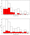 |
Fig. 1. Top: Spectral types of Bsgs with OGLE data (red) and the total number of Bsgs from our sample (solid line). Bottom: Recovery fraction for Gaia multi-epoch photometry. Known LBVs are not shown. |
2.2. OGLE multi-epoch photometry
The Optical Gravitational Lensing Experiment (OGLE) survey provides high-cadence photometry in the Cousins I band, with observations spanning approximately June 2001 to 2020, depending on the data release. The cadence varies from a few days to weekly sampling, depending on field and observing season, and the data were obtained using the 1.3 m Warsaw telescope at Las Campanas Observatory in Chile. The median FWHM of the OGLE imaging is approximately 1″, providing sufficient spatial resolution to resolve individual massive stars in the LMC. We refer to Udalski et al. (2015) and references therein for further details on the survey and data reduction.
We cross-matched these known BSgs with multi-epoch photometry from the OGLE-IV survey using a radius of 1″. In cases where OGLE-IV data were unavailable, we supplemented the sample with OGLE-III data, which provide shorter temporal coverage (Udalski 2003). A total of 83 unique matches were found in the OGLE-IV dataset and 6 in the OGLE-III dataset. The OGLE dataset for each source contain typically around a thousand epochs per star, with coverage extending over nearly two decades. This enables the detection of variability phenomena on short and long timescales. The photometric precision in the I band is on the order of 0.01 mag for unsaturated sources and systematics are minimized through the use of difference image analysis (Wozniak 2000).
2.3. Gaia DR3 multi-epoch photometry
Gaia DR3 includes multi-epoch photometry for selected bright sources (Eyer et al. 2023). This covers observations across the custom GaiaG, BP, and RP filters spanning July 2014 to May 2017, covering between 30–80 epochs per target (except for Sk −66°185, which has 175 epochs). Multi-epoch photometry was retrieved using the PYTHON astroquery package, with only photometric points satisfying the variability_flag_g_reject (and in the respective filters for color analysis) retained. We also ensured there were at least 25 epochs for source for the analysis. In total, there were 49 BSgs with Gaia DR3 multi-epoch photometry, with 11 of these also having OGLE IV light curves and 1 having an OGLE III light curve. We also retrieved the light curves of all confirmed LBVs (seven sources) from Richardson & Mehner (2018), which were not included in our input catalog from Bonanos et al. (2009). The analysis of these light curves are in Appendix A.
2.4. Recovery and completeness
Figure 1 also shows the recovery fraction of BSgs in OGLE, and Gaia DR3 as a function of spectral subtype. We find that approximately 36% of the BSgs identified by Bonanos et al. (2009) have light curves in the OGLE datasets. For OGLE, this is mostly because of saturation, given the saturation limit around 12 mag in V. This limit excludes all known LBVs in the LMC, which have apparent magnitudes brighter than ∼12 mag in the optical (Richardson & Mehner 2018). We note that for B supergiants, on average, the magnitude stays relatively the same, or slightly increases with decreasing spectral class (for early Bs, from B0-B3 between 11–14 mag; and for latter types between 10–13 mag). A few objects fall into CCD gaps and, thus, they were not recovered. For the Gaia dataset, the recovery fraction is dependent on a variety of factors and is expected to increase significantly in future releases (Eyer et al. 2023).
The total fraction of stars with light curves is ∼49% and this sample is biased towards earlier spectral types due to the OGLE dataset; however, a few latter spectral types are recovered from the Gaia photometry. For this sample size, simple binomial properties can be estimated at the 99% confidence level with a 8% margin of error given the total sample size. We note that while our selection criteria are biased due to the saturation (and faintness) limit of the photometry, considering the B spectral class as a whole, the data reflect a sufficiently representative sample for such an analysis. The list of 126 unique BSgs analyzed and their properties are electronically available via CDS, along with the complete list of 254 BSgs that are shown in Fig. 1. An representative of this is shown in Table 1.
B supergiants in the LMC.
3. Analysis of time series data
3.1. δm − δt histograms
To examine aperiodic variability, we computed the δm − δt plot for each light curve as described in Kalari et al. (2018), which represents the incidence of variability at a particular timescale in a light curve. It is defined as the sum of all observations at magnitude, m, and time, t, of a light curve, by computing the differences,
 (1)
(1)
where i > j such that each pair is only considered once. By presenting the differences between magnitude and time as a density histogram, we can directly observe how much variability is observed on what timescales. BSgs with δm greater than 0.1 mag were examined visually. The resulting δm − δt plots for all sources are provided on request to the principal author. A representative example using OGLE and Gaia data are given in Fig. 2.
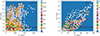 |
Fig. 2. Representative example of the time series photometric analysis, where the color gradient marks the density of the points. Left: LBV candidate [ST92] 4-13 δm − δt histogram computed using OGLE-IV data, with the δm levels of 0.08 (10σ) and 0.1 mag marked. Right: Same as the left, but for the known LBV HD 269216, computed from Gaia multi-epoch photometry. |
From the δm − δt plots, we only identified three stars with OGLE data that show aperiodic variability above the significance threshold. The first is [ST92] 4-13 (alias W61 4-1 in SIMBAD1, and Gaia DR3 4657649594536852352), a B1 I star, with the magnitude changing by nearly 1 mag over the past two decades. The other two are VFTS 698, the known binary masquerading as a B[e] star (Dunstall et al. 2012), and VFTS 652– a known spectroscopic double lined binary (Howarth et al. 2015). We discarded these two from our sample given that the magnitudes vary by less than 0.5 mag over the timescale. We only considered [ST92]4-13, as binarity is likely to be the origin of the magnitude variations in the latter two.
In the Gaia dataset, there is only one star with the δm − δt histogram resembling a S Dor variable. HD 269216 (HIP 24347, Gaia DR3 4658204053297963392) is a known LBV, previously identified in Prinja & Schild (1991) and Walborn et al. (2017). Eight other stars do show aperiodic variability above 0.1 mag, but not at significant levels as those seen in [ST92]4-13 or HD 269216 (i.e. < 0.5 mag). This variability depends on a few (< 5) epochs when examining the light curves and given the scan-dependent possibility of spurious signals (Holl et al. 2023), we refrain from examining these further without future epoch photometry confirming the variability.
3.2. von Neumann η index
In addition to the δm − δt histograms, a method for identifying irregular variability in irregularly spaced data is via the von Neumann index (Shin et al. 2009). This index is computed as the mean squared successive difference over the variance of the distribution and acts as an indicator of independence for a series of observations (von Neumann 1941). In photometric monitoring observations, it allows us to identify whether the underlying distribution is smooth. We adopted the 1/η value, as defined in Sokolovsky et al. (2017), as a variability indicator, where larger values indicate irregular variability.
Our analysis results are shown in Fig. 3. Here, the histogram of 1/η values for our sample is shown in logarithmic scale, computed for both the Gaia and OGLE light curves. Three stars in the OGLE sample display values that are 3σ away from the mean of the Gaussian fitted to the distribution (peaking at μ = −0.15 in log scale). These are [ST92] 4-13 with a log(1/η) value of 1.81, LH 104 4-67 (1.13), and LH 101 5-18 (1.18). On examining the light curve of the latter two, we find that a jump between epochs in the mean magnitude, rather than any aperiodic behavior causes these high values. In the Gaia dataset, HD 269216 shows a value discrepant from the median of 1.11. Overall, a comparison with the von Neumann index suggests that the same stars would have been identified for aperiodicity. The functions used to compute both the δm − δt histograms and the von Neumann η index are publicly available2.
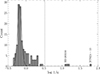 |
Fig. 3. Histogram of 1/η values computed using OGLE and Gaia light curves, in logarithmic scale. The positions of the identified LBVs, HD 269216, and [ST92] 4-13 are marked. The best-fit Gaussian to the population except the outliers (log (1/η) > 1) is shown by the dashed line. The dotted line shows the 3σ cut-off. |
4. The S Dor variables: [ST92] 4-13 and HD 269216
4.1. [ST92] 4-13
4.1.1. Photometric variability
In Fig. 4, we show the light curve of the candidate S Dor variable–[ST92] 4-13, spanning nearly two decades. The light curve displays oscillations on the timescales of few months and the brightness decreased by 0.7 mag from 13 June 2009 to May 2012 and then increased with a larger oscillation range. In the Lomb-Scargle periodogram, we found at least four significant peaks: three of around a few days and a longer one at seven years. Large amplitude variations have ceased since 2022. Figure 4 visualizes the aperiodic change seen, showing a magnitude increase of nearly 0.8 mag seen over timescales of a year. The nearly yearly period seen along with the large amplitude variations are consistent with the changes seen for S Dor variables van Genderen (2001). For instance, van Genderen (2001) reported a period of 371.4 days for AG Car with beat cycles. Gaia indicators of multiplicity (RUWE and ipd_fmp) that have recovered binaries in early emission line B-type stars (Kalari et al. 2025) do not indicate that there is an unseen companion that may cause the observed light curve. Based on this information, we classified [ST92] 4-13 as a S Dor variable. We note that further unreleased OGLE observations taken between 2020-2024, which were not part of the original analysis were examined for [ST92] 4-13 and are shown in Fig. 4.
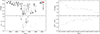 |
Fig. 4. Left: I-band light curve of [ST92] 4-13, with the (V − I) color shown at the bottom. Data are from the OGLE-IV photometry. The red asterisk marks the epoch when the spectral data were taken. Right: GaiaG and (BP − RP) magnitude and color light curves of HD 269216, shown at the top and bottom panel respectively. |
4.1.2. Spectral analysis
Investigating whether there might be spectral changes accompanying the aperiodic light curve seen here, we searched the literature for for spectra. Schild & Testor (1992) noted it as having (B − V) of −0.09 and (U − B) of −0.82, with data taken between 1988 and 1990, and a spectral type of B1 Ia based on low resolution spectroscopic observations using the He Iλ4471/Mg IIλ4481 and He Iλ4144/He Iλ4121 line ratios within the same time frame. The object is marked as an emission line star based on the catalog of Howarth (2013); however, no line widths have been provided. Gaia DR3 (Gaia Collaboration 2023) XP mean spectra (reference epoch 2016.0) of the object shows a corrected Hα line width of −15 Å.
To observe whether any changes in spectral type are seen, we obtained spectra using the Gemini high-resolution optical spectrograph (GHOST) at Gemini South (Kalari et al. 2024), on November 10, 2024 (epoch marked in Fig. 4; MJD of 60624.210). Data were taken in photometric conditions with seeing around 0.8″. Immediately after the science target, we observed the spectrophotometric standard for CPD-69 177 for absolute flux calibration. The final spectra are characterized by R∼ 47 000, reaching signal-to-noise ratios (S/Ns) around 50 near the V band. The spectra display prominent Balmer emission lines, which consist of a broad and narrow emission component. The effective temperature is more representative of late-B type supergiant from the spectra, with changes observed in the Hα line width compared to the Gaia spectrum (−20Å). The Balmer profiles do not exhibit the P Cygni morphology in the lower H lines seen in LBV candidates during quiescence (as shown in Massey et al. 2007). This is in line with the prediction that the object is heading towards visual minimum in the light curve. However, the Balmer profiles do show a P Cygni profile in He I.
To estimate the stellar parameters of [ST92] 4-13 and get an idea of its evolutionary status, we used the genetic algorithm KIWI-GA (Brands et al. 2022) in combination with the stellar atmosphere code FASTWIND (v10.6; Santolaya-Rey et al. 1997; Puls et al. 2005; Rivero González et al. 2012; Carneiro et al. 2016; Sundqvist & Puls 2018). We describe the spectral reduction process and modeling approach in Appendix B. For a more in-depth explanation of the models, we refer to the cited literature. In brief, KIWI-GA is a Python wrapper for FASTWIND that uses the concept of evolution to automatically fit FASTWIND models to an observed spectrum. Over a predefined number of generations and number of individuals per generation, the desired parameter space is explored by means of reproduction and mutation to find, for a given input spectrum, the best fitting stellar and wind parameters and statistical uncertainties. Here, we used 81 generations with 85 models per generation to estimate the stellar parameters of our target star.
The best-fitting parameters are given in Table 2, with the corresponding best-fitting spectrum and parameter posteriors shown in Fig. 5. The top four rows of the figure show the observed, continuum-normalized spectrum, and error bars in black, the best fitting FASTWIND model as the solid green line, and the 1σ uncertainty region as the shaded green region. The bottom three rows show the posteriors for each free parameter. On each of these axes, the points represent the models of the KIWI-GA run, whose colors are mapped to the generation number of the model. The red vertical line gives the best fitting value, while the dark and light yellow shaded regions give the 1- and 2σ uncertainty regions, respectively.
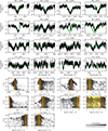 |
Fig. 5. KIWI-GA fit of [ST92] 4-13. See Sect. 4.1.2 for details. |
Best-fitting parameters and 1σ uncertainties for [ST92] 4-13 determined by KIWI-GA.
For [ST92] 4-13, we estimate an effective temperature Teff ≃ 17 kK and surface gravity log(g/cm s−2)≃1.9. To compute the extinction and luminosity, we drew from the VI photometry from August 19, 2022 (the closest multi-band photometry to the epoch of spectroscopic observations) of V = 14.305 and I = 13.931. We can also justify this assumption based on the fact that the I magnitude is very similar to the epoch of spectroscopic observations (I = 13.927 on November 10, 2024). Computing a bolometric correction in I of −1.76 and a model (V − I)model of −0.15, we arrived at an AI of 0.77, leading to log (L/L⊙) of 4.73 dex.
As an alternative means of computing the luminosity, we rescaled the spectral energy distribution of the best-fitting FASTWIND model to the aforementioned I magnitude, adopting a distance modulus to the LMC of 18.48 (Pietrzyński et al. 2019) and accounting for the I band extinction given above. This rescaling results in log (L/L⊙) of 4.57 dex. We therefore quoted an average value of the luminosity of [ST92] 4-13 as 104.6 ± 0.15 L⊙, where the uncertainties capture the discrepancies between the two methods. The object is shown on a Hertzsprung-Russell diagram, along with known LBVs from the literature in Fig. 6.
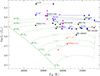 |
Fig. 6. Location in the HRD of [ST92] 4-13 based on Schild & Testor (1992, left), with the current observations (right) are shown in red. The positions of confirmed LBVs from the literature in the galaxy (black circles), LMC (blue circles), and the SMC (orange circle; including AzV 261, discussed in Sect. 5.1) are also shown. Magenta circles marks the position of known LBVs in M31 and M33 (from Humphreys et al. 2017a). The dashed green lines are the stellar tracks from Brott et al. (2011) with the corresponding initial stellar mass indicated, and the solid line is the zero-age main sequence isochrone for LMC metallicity. |
4.1.3. Classification and evolutionary status of [ST92] 4-13
The spectroscopic analysis points to change in spectral type compared to the literature, from B1a (Schild & Testor 1992) to approximately B2.5 (a change in Teff of around 5kK based on the scale of Trundle et al. 2007). However, the derived luminosity is nearly an order of magnitude lower than that of the population of known LBVs Smith et al. (2004). The star does exhibit an infrared (IR) Ca II triplet, as typically seen in LBVs, but not the forbidden [Ca II] emission or any forbidden lines seen in B[e] stars, as discussed by Humphreys et al. (2017b); it does not exhibit not the classic P Cygni profiles of LBVs in this stage either. The object is also not detected at longer wavelengths, ruling out a hot post-asymptotic giant branch (pAGB) classification (e.g. see the discussion of the potential hot pAGB/LBV star WRA 571 in Garcia-Lario et al. 1998) or even a B[e] classification (which have hot dust discs in the LMC; e.g. Kraus 2019; Kalari et al. 2014). Furthermore, there is no object currently known that would exhibit these S Dor variations other than LBVs. However, based on its low luminosity and lack of P Cygni profiles in its spectra, we consider the status of [ST92] 4-13 as a LBV to be ambiguous.
4.2. HD 269216: Photometric and spectroscopic variability
HD 269216 was first proposed as a LBV candidate on the basis of ultraviolet and optical spectra by Prinja & Schild (1991). Later, Walborn et al. (2017) compiled archival photometric and spectroscopic information detailing the outburst between 2014 and 2016, where the spectrum changed from a late-B supergiant towards an A-F type supergiant. We concur with this analysis based on the Gaia light curve, which has shown that the object has brightened considerably during the 2014–2016 outburst and is continuing that trend. Further monitoring of this object can track whether it has brightened since late 2020.
4.3. Circumstellar dust
Overall, LBVs show evidence of excess free-free emission (Humphreys et al. 2017b,a), similar to classical Be stars, and not containing a warm dust component as found in other LBV-like objects such as B[e] stars. In Fig. 7, we show the near-IR (J − H) versus (H − Ks) color-color diagram displaying the position of known massive stars, as well as [ST92] 4-13 and HD 269216. In addition, we also show the data in the mid-IR from WISE. In these diagrams, [ST92] 4-13 exhibits modest free-free emission at levels similar to other known S Dor LBVs. HD 269216; however, resembles most main sequence massive stars and we note that both resemble the colors of known LBVs (Humphreys et al. 2017b).
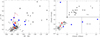 |
Fig. 7. Left: Near-IR (J − H) vs. (H − Ks) color-color diagram of known sgB[e] (open squares), warm hypergiants (open triangles), cBe stars (open circles), known S Dor variables (blue dots), BSgs (small dots), and [ST92] 4-13, HD 269216 (red asterisks). Data taken from Humphreys et al. (2017b). The dashed red line is the main-sequence locus. Right: Mid-IR [3.6 μm]–[4.5 μm] vs. [5.8 μm]–[8.0 μm] color-color diagram. |
5. Discussion
5.1. S Dor variability and LBV classification
In the literature, it is common practice to refer to massive stars with major (of which are only η Car, P Cyg) or minor outbursts (for e.g. S Dor) as LBVs. The latter are often characterized as S Dor variables (after their namesake), but they are often clumped together as bona fide LBVs. LBV candidates (LBVc), on the other hand are those having spectroscopic features (e.g. deep P Cygni profiles, spectroscopic transitions between late and early supergiants, etc.), but not the accompanying photometric variations at the S Dor level.
In this paper, as well as in Kalari et al. (2018), we searched for evidence of S Dor variability among the BSg population in the LMC (and in the SMC in the earlier work). We found evidence of one candidate in the SMC which showed S Dor type variability without any spectral changes. Here, we show another candidate [ST92],4-13 in the LMC which demonstrates similar S Dor type variability over 20 years, but is likely not an LBV.
This brings us to the key questions of our study. For instance, we considered whether S Dor-like photometric variations unique to LBVs and where we might classify S Dor like photometric variability without the accompanying spectral variations, as in the case of the objects discussed here. Weis & Bomans (2020), Conti (1997) laid out the defining characteristic of LBVs, which is the S Dor variability or (in extremely rare cases) an η-Car like outburst. Here, we show evidence for two S Dor type variables, but with luminosity and spectral characteristics that do not resemble known LBVs.
Potential hints can be drawn from the detection of known double-lined binaries, VFTS,698 and VFTS,652 as irregular variables in our analysis, albeit with amplitudes lower than the classical S Dor variables. The former demonstrated long-term variability, but also a B[e] spectrum (and IR colors) and it was classified as W-Serpentis variable, consisting of a massive binary around a cool primary. The latter was classified as a Algol-type variable, with a low-mass primary. Compared to these two, both AzV 261 and [ST92] 4-13 are single-lined (latter a binary based on multi-epoch radial velocity variations in the He I line). It is possible that mass transfer across binary components could lead in specific cases to S Dor like light curves, such as that seen in AzV 261 (Bodensteiner et al. 2025) or [ST92] 4-13. Further high-resolution multi-epoch spectra of both these sources are necessary to understand the origin of these variations and whether they can be attributed to binary mass transfer or if they are accompanied by spectral type changes. It might also be the case that most LBVs are born from mergers of hierarchical triple systems (Hirai et al. 2021) and the two stars discussed here could be the lower mass counterparts of such interactions. With the advent of multi-epoch photometry from surveys such as LSST, care must be taken in defining the variability of LBVs based on photometric variability. In this case, LBV should only be classified as such when observed with accompanying spectral characteristics. Drawing from the duck analogy laid out in Conti (1997) and Massey et al. (2007), we suggest that if an LBV shows photometric and spectroscopic variability, it should be classified as an LBV; and if only shows one or the other, it should be classified as a LBVc.
An alternative explanation for [ST92] 4-13 and AzV 261 could be that these objects are the observational indication of low-luminosity LBVs (Smith et al. 2004). It has been proposed using rotating evolutionary models (Levesque et al. 2025; Meynet & Maeder 2005) that stellar rotation lowers the mass (and thereby luminosity) threshold of the LBV phase. At solar metallicities, this is predicted to be around 22 M⊙, although the mass limit is thought to increase at lower metallicities and to be dependent on the rotational velocity.
At LMC metallicity, for an initial velocity of 300 km s−1, Meynet & Maeder (2005) found a lower initial mass limit of 25 M⊙. The initial mass of [ST92] 4-13 is lower than this limit; hence, we considered this possibility to be unlikely. Instead, we considered that the examples of the S Dor type phenomena at even lower luminosities (and by inference lower masses) reported here and in Kalari et al. (2018) might not actually be linked to a single evolutionary phase; rather, they could be caused by Eddington-limit related physics at a range of masses, which could involve certain processes such as binary evolution.
5.2. S Dor variables among the Bsg population
The primary motivation of our study was to follow up on our previous results presented Kalari et al. (2018), but with a longer baseline and to cover a large sample size by studying BSgs in the LMC. In that study, based in the SMC, over a three-year baseline observation of 64 BSgs, we detected only one potential S Dor variable (AzV 261), which did not show any spectral type variation. Here, covering a sample size of 87 (37) across a 20 (3) year timescale, we found two objects exhibiting S Dor-type variations. One was the known LBV, HD 269216 and the other was the newly identified S Dor variable [ST92] 4-13. The latter exhibits a potential change in spectral type from B1 (literature) to B2.5, but its luminosity is too low to be classified as an LBV. In addition, its spectra do not show the P Cygni profiles caused due to strong mass loss of LBVs.
Under the assumption that all known LBVs have been discovered from the Bsgs population of the LMC galaxy (8, and 4 candidate S Dor variables from 250 known Bsgs according to census compiled by Bonanos et al. 2009), we estimate the duty cycle of the S Dor phase to be at most ∼few 103 yr (assuming a He-burning lifetime of 105 years). This is similar to the value found for the SMC (Kalari et al. 2018).
The prior work carried out on the SMC was based on multi-epoch photometry covering a three-year baseline. In the present study, we expanded the baseline and sample size. The similarity of the duty cycle estimated by the two studies at different metallicity values suggest that, based on the current observational limitations in magnitude range and baselines, the S Dor duty cycle is at least an order of magnitude shorter than commonly assumed. Moreover, BSgs and LBVs are truly different evolutionary stages in the life-cycle of massive stars. In other words, we find that BSgs are not dormant LBVs.
6. Conclusions
Here, we have improved on previous searches for LBV variability among BSgs by increasing the baseline and sample size from the previous work of Kalari et al. (2018). We examined the 20-year nearly nightly cadence light curves of 87 BSgs from OGLE, along with the 3-year Gaia multi-epoch photometry of 37 BSgs in the LMC. As a result, we found evidence for S Dor-type variability found in LBVs for one known LBV (HD 269216) and one BSg ([ST92] 4-13). Our conclusions are listed below.
-
Despite an increased sample size and baseline, the duty cycle we found for LBVs was roughly similar at around 103 years. This suggests that LBVs are truly unique or transitory objects and it is unlikely for the LBV phenomenon to be widespread among the general BSg population.
-
We also argue that both photometric and spectral type variations, along with spectral characteristics and high-luminosities are necessary to classify LBVs, based on the properties of the candidates presented here.
-
Our findings suggest that LBV-like variability is a physical phenomena and not and not solely linked to any one particular evolutionary phase.
Our study in the LMC agrees with previous findings in the SMC that the duty cycle of LBVs is around 103 years, and that LBVs appear to be unique, transitory objects rather than dormant BSgs. The discovery of LBV-like photometric variability in stars that do not show other LBV characteristics suggests that the variability is a physical phenomenon rather than an evolutionary one.
Data availability
The full Table 1 is available at the CDS via https://cdsarc.cds.unistra.fr/viz-bin/cat/J/A+A/708/A343
Acknowledgments
V. M.K. is supported by the international Gemini Observatory, a program of NSF NOIRLab, which is managed by the Association of Universities for Research in Astronomy (AURA) under a cooperative agreement with the U.S. National Science Foundation, on behalf of the Gemini partnership of Argentina, Brazil, Canada, Chile, the Republic of Korea, and the United States of America. The OGLE project has received funding from the Polish National Science Centre grant OPUS-28 2024/55/B/ST9/00447 to AU. This work presents results from the European Space Agency (ESA) space mission Gaia. Gaia data are being processed by the Gaia Data Processing and Analysis Consortium (DPAC). Funding for the DPAC is provided by national institutions, in particular the institutions participating in the Gaia MultiLateral Agreement (MLA). The Gaia mission website is https://www.cosmos.esa.int/gaia. The Gaia archive website is https://archives.esac.esa.int/gaia. This research has made use of the SIMBAD database, CDS, Strasbourg Astronomical Observatory, France.
References
- Bodensteiner, J., Shenar, T., Sana, H., et al. 2025, A&A, 698, A38 [NASA ADS] [CrossRef] [EDP Sciences] [Google Scholar]
- Bonanos, A. Z., Massa, D. L., Sewilo, M., et al. 2009, AJ, 138, 1003 [Google Scholar]
- Brands, S. A., de Koter, A., Bestenlehner, J. M., et al. 2022, A&A, 663, A36 [Google Scholar]
- Brott, I., de Mink, S. E., Cantiello, M., et al. 2011, A&A, 530, A115 [NASA ADS] [CrossRef] [EDP Sciences] [Google Scholar]
- Carneiro, L. P., Puls, J., Sundqvist, J., & Hoffmann, T. 2016, A&A, 590, A88 [NASA ADS] [CrossRef] [EDP Sciences] [Google Scholar]
- Conti, P. S. 1997, in Luminous Blue Variables: Massive Stars in Transition, eds. A. Nota, & H. Lamers, ASP Conf. Ser., 120, 387 [NASA ADS] [Google Scholar]
- Dunstall, P. R., Fraser, M., Clark, J. S., et al. 2012, A&A, 542, A50 [NASA ADS] [CrossRef] [EDP Sciences] [Google Scholar]
- Eyer, L., Audard, M., Holl, B., et al. 2023, A&A, 674, A13 [NASA ADS] [CrossRef] [EDP Sciences] [Google Scholar]
- Gaia Collaboration (Vallenari, A., et al.) 2023, A&A, 674, A1 [NASA ADS] [CrossRef] [EDP Sciences] [Google Scholar]
- Garcia-Lario, P., Riera, A., & Manchado, A. 1998, A&A, 334, 1007 [NASA ADS] [Google Scholar]
- Grassitelli, L., Langer, N., Mackey, J., et al. 2021, A&A, 647, A99 [NASA ADS] [CrossRef] [EDP Sciences] [Google Scholar]
- Hirai, R., Podsiadlowski, P., Owocki, S. P., Schneider, F. R. N., & Smith, N. 2021, MNRAS, 503, 4276 [NASA ADS] [CrossRef] [Google Scholar]
- Holl, B., Fabricius, C., Portell, J., et al. 2023, A&A, 674, A25 [NASA ADS] [CrossRef] [EDP Sciences] [Google Scholar]
- Howarth, I. D. 2013, A&A, 555, A141 [NASA ADS] [CrossRef] [EDP Sciences] [Google Scholar]
- Howarth, I. D., Dufton, P. L., Dunstall, P. R., et al. 2015, A&A, 582, A73 [NASA ADS] [CrossRef] [EDP Sciences] [Google Scholar]
- Humphreys, R. M., Davidson, K., Hahn, D., Martin, J. C., & Weis, K. 2017a, ApJ, 844, 40 [Google Scholar]
- Humphreys, R. M., Gordon, M. S., Martin, J. C., Weis, K., & Hahn, D. 2017b, ApJ, 836, 64 [NASA ADS] [CrossRef] [Google Scholar]
- Justham, S., Podsiadlowski, P., & Vink, J. S. 2014, ApJ, 796, 121 [NASA ADS] [CrossRef] [Google Scholar]
- Kalari, V. M., Vink, J. S., Dufton, P. L., et al. 2014, A&A, 564, L7 [NASA ADS] [CrossRef] [EDP Sciences] [Google Scholar]
- Kalari, V. M., Vink, J. S., Dufton, P. L., & Fraser, M. 2018, A&A, 618, A17 [NASA ADS] [CrossRef] [EDP Sciences] [Google Scholar]
- Kalari, V. M., Diaz, R. J., Robertson, G., et al. 2024, AJ, 168, 208 [Google Scholar]
- Kalari, V. M., Salinas, R., Saez-Carvajal, C., et al. 2025, ApJ, 993, 192 [Google Scholar]
- Kotak, R., & Vink, J. S. 2006, A&A, 460, L5 [NASA ADS] [CrossRef] [EDP Sciences] [Google Scholar]
- Kraus, M. 2019, Galaxies, 7, 83 [NASA ADS] [CrossRef] [Google Scholar]
- Levesque, E. M., Lamers, H. J. G. L. M., & de Koter, A. 2025, ApJ, 981, 176 [Google Scholar]
- Massey, P., McNeill, R. T., Olsen, K. A. G., et al. 2007, AJ, 134, 2474 [NASA ADS] [CrossRef] [Google Scholar]
- McErlean, N. D., Lennon, D. J., & Dufton, P. L. 1999, A&A, 349, 553 [NASA ADS] [Google Scholar]
- Meynet, G., & Maeder, A. 2005, A&A, 429, 581 [CrossRef] [EDP Sciences] [Google Scholar]
- Pietrzyński, G., Graczyk, D., Gallenne, A., et al. 2019, Nature, 567, 200 [Google Scholar]
- Prinja, R. K., & Schild, H. 1991, A&A, 249, 428 [NASA ADS] [Google Scholar]
- Puls, J., Urbaneja, M., Venero, R., et al. 2005, A&A, 435, 669 [NASA ADS] [CrossRef] [EDP Sciences] [Google Scholar]
- Richardson, N. D., & Mehner, A. 2018, Res. Notes Am. Astron. Soc., 2, 121 [Google Scholar]
- Rivero González, J., Puls, J., Najarro, F., & Brott, I. 2012, A&A, 537, A79 [NASA ADS] [CrossRef] [EDP Sciences] [Google Scholar]
- Santolaya-Rey, A. E., Puls, J., & Herrero, A. 1997, A&A, 323, 488 [NASA ADS] [Google Scholar]
- Schild, H., & Testor, G. 1992, A&AS, 92, 729 [NASA ADS] [Google Scholar]
- Shin, M.-S., Sekora, M., & Byun, Y.-I. 2009, MNRAS, 400, 1897 [NASA ADS] [CrossRef] [Google Scholar]
- Skiff, B. A. 2009, CDS/ADC Collection of Electronic Catalogues, 1, 2023 (2009) [Google Scholar]
- Smith, N. 2007, in Supernova 1987A: 20 Years After: Supernovae and Gamma-Ray Bursters, eds. S. Immler, K. Weiler, & R. McCray, AIP Conf. Ser., 937, 163 [Google Scholar]
- Smith, N., Vink, J. S., & de Koter, A. 2004, ApJ, 615, 475 [NASA ADS] [CrossRef] [Google Scholar]
- Sokolovsky, K. V., Gavras, P., Karampelas, A., et al. 2017, MNRAS, 464, 274 [CrossRef] [Google Scholar]
- Sundqvist, J., & Puls, J. 2018, A&A, 619, A59 [NASA ADS] [CrossRef] [EDP Sciences] [Google Scholar]
- Testor, G., & Niemela, V. 1998, A&AS, 130, 527 [NASA ADS] [CrossRef] [EDP Sciences] [Google Scholar]
- Tombleson, R., & Smith, N. 2015, Am. Astron. Soc. Meeting Abstr., 225, 343.17 [Google Scholar]
- Trundle, C., Dufton, P. L., Hunter, I., et al. 2007, A&A, 471, 625 [NASA ADS] [CrossRef] [EDP Sciences] [Google Scholar]
- Trundle, C., Kotak, R., Vink, J. S., & Meikle, W. P. S. 2008, A&A, 483, L47 [NASA ADS] [CrossRef] [EDP Sciences] [Google Scholar]
- Udalski, A. 2003, Acta Astron., 53, 291 [NASA ADS] [Google Scholar]
- Udalski, A., Szymański, M. K., & Szymański, G. 2015, Acta Astron., 65, 1 [NASA ADS] [Google Scholar]
- van Genderen, A. M. 2001, A&A, 366, 508 [NASA ADS] [CrossRef] [EDP Sciences] [Google Scholar]
- van Genderen, A. M., & Sterken, C. 1999, A&A, 349, 537 [NASA ADS] [Google Scholar]
- von Neumann, J. 1941, Ann. Math. Stat., 12, 367 [Google Scholar]
- Walborn, N. R., Gamen, R. C., Morrell, N. I., et al. 2017, AJ, 154, 15 [NASA ADS] [CrossRef] [Google Scholar]
- Weis, K., & Bomans, D. J. 2020, Galaxies, 8, 20 [NASA ADS] [CrossRef] [Google Scholar]
- Wozniak, P. R. 2000, Acta Astron., 50, 421 [NASA ADS] [Google Scholar]
Bonanos et al. (2009) and SIMBAD list W61 4-1 as B1 Ia based on Testor & Niemela (1998). However, this is likely to be an incorrect reference, as that paper does not include any stars from this cluster. The spectral type based on those coordinates appears to be based on the result of Schild & Testor (1992), where it is classified as star 4-13 in the cluster LH104; hence, we adopted [ST92] 4-13 as the reference name. See also Skiff (2009).
Appendix A: δm − δt histograms and η index of confirmed LMC LBVs
We retrieved Gaia DR3 multi-epoch photometry of confirmed LBVs listed in Richardson & Mehner (2018, see Sect. 2.3). There are seven sources, all of which had multi-epoch photometry spanning the DR3 period (3 years). We show in Fig. A.1 the histograms computed as described in Sect. 3.1, utilizing the G-band photometry. Only data points with variability_flag_g_reject=False were used in any analysis. The histograms all have aperiodic variability above the significance level. The distribution of the histograms are similar to the LBV HD 269216 and [ST92] 4-13, but the histogram of [ST92] 4-13 also shows a periodic trend along with aperiodic variability (both vertical and inclined lines).
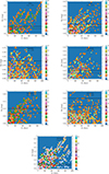 |
Fig. A.1. δm − δt histograms of confirmed LMC LBVs, with the 1/η value given in the top right. |
In the top-right of each histogram, the 1/η index is given, and computed as described in Sect. 3.2. All stars have significant indexes except for HD 269700, representative of aperiodic variability. The lack of variability is not surprising for HD 269700, since it is considered an ex/dormant LBV (van Genderen & Sterken 1999). All these stars would be selected as an LBV with our analysis methodology, indicating our method is suitable to recover LBVs. Future multi-epoch photometry from Gaia3 covering a much larger baseline can be used to search for further possible LBVs in the Magellanic Clouds.
Appendix B: Modeling approach for [ST92] 4-13
In this section, we describe how we prepared the optical spectrum of [ST92] 4-13 to be analyzed. First, we decided on a list of diagnostic spectral lines. With the main goal of this exercise being to gauge the evolutionary status of our target, we are primarily interested in the determination of the effective temperature (Teff) and surface gravity (g) from its spectrum, along with the luminosity (L) from these. For Teff, we used the Si II to Si III ratio; the primary temperature diagnostic in B stars (e.g. McErlean et al. 1999). We used the photospheric He I lines to constrain g. As these lines show wind features, we also use them to get an idea of the mass loss rate (Ṁ) and terminal wind speed (v∞). Regarding the wind structure, we assumed a fixed clumping factor of 10 and that all clumps in the wind are optically thin. We also estimate the projected rotational velocity, v sin i. We do not account for macroturbulent broadening here, so our quoted value of  km s−1 in Table 2 is an upper limit of the true projected rotational velocity. Finally, we left the helium abundance (YHe := NHe/NH), and C, N, O, and Si abundances as free parameters in our fit.
While the spectrum of our target exhibits strong Balmer emission, indicative of a dense stellar wind, we do not fit these lines here. Our current assumptions regarding the wind structure are not enough to adequately describe the nature of the stellar wind; simultaneous modelling of the UV spectrum, where resonance lines of metals lie, would be needed to gain a complete picture of the wind of this star. From a test run where the Balmer lines were included, we found they strongly biased Teff and g to very high values to compensate for our assumptions regarding the wind structure, resulting in an overall very poor fit. In any case, we are not interested in studying Ṁ here, so we left them out for these reasons.
FASTWIND and KIWI-GA requires a radial velocity-corrected, continuum-normalised spectrum as input. To correct for the radial velocity, we performed a cross-correlation using a template of Gaussian absorption profiles at the wavelengths of the photospheric He I profiles, as well as at the three components of the Si IIIλ4452 profile. From this we find a radial velocity of 269 ± 38 km s−1.
Once corrected for radial velocity, we locally normalised the target spectral lines. For a given line, this involved masking spectral features blue and red of the line, fitting a line through the local continuum level, and dividing through by this line. This is a reasonable approach given the relatively few spectral lines in the optical spectrum. In some instances, it was necessary to fit degree 2 polynomials to the continuum. This was the case for C IIIλ4070, He Iλ4143, and the O II doublet at 4416 Å.
All Tables
Best-fitting parameters and 1σ uncertainties for [ST92] 4-13 determined by KIWI-GA.
All Figures
|
Fig. 1. Top: Spectral types of Bsgs with OGLE data (red) and the total number of Bsgs from our sample (solid line). Bottom: Recovery fraction for Gaia multi-epoch photometry. Known LBVs are not shown. |
| In the text | |
|
Fig. 2. Representative example of the time series photometric analysis, where the color gradient marks the density of the points. Left: LBV candidate [ST92] 4-13 δm − δt histogram computed using OGLE-IV data, with the δm levels of 0.08 (10σ) and 0.1 mag marked. Right: Same as the left, but for the known LBV HD 269216, computed from Gaia multi-epoch photometry. |
| In the text | |
|
Fig. 3. Histogram of 1/η values computed using OGLE and Gaia light curves, in logarithmic scale. The positions of the identified LBVs, HD 269216, and [ST92] 4-13 are marked. The best-fit Gaussian to the population except the outliers (log (1/η) > 1) is shown by the dashed line. The dotted line shows the 3σ cut-off. |
| In the text | |
|
Fig. 4. Left: I-band light curve of [ST92] 4-13, with the (V − I) color shown at the bottom. Data are from the OGLE-IV photometry. The red asterisk marks the epoch when the spectral data were taken. Right: GaiaG and (BP − RP) magnitude and color light curves of HD 269216, shown at the top and bottom panel respectively. |
| In the text | |
|
Fig. 5. KIWI-GA fit of [ST92] 4-13. See Sect. 4.1.2 for details. |
| In the text | |
|
Fig. 6. Location in the HRD of [ST92] 4-13 based on Schild & Testor (1992, left), with the current observations (right) are shown in red. The positions of confirmed LBVs from the literature in the galaxy (black circles), LMC (blue circles), and the SMC (orange circle; including AzV 261, discussed in Sect. 5.1) are also shown. Magenta circles marks the position of known LBVs in M31 and M33 (from Humphreys et al. 2017a). The dashed green lines are the stellar tracks from Brott et al. (2011) with the corresponding initial stellar mass indicated, and the solid line is the zero-age main sequence isochrone for LMC metallicity. |
| In the text | |
|
Fig. 7. Left: Near-IR (J − H) vs. (H − Ks) color-color diagram of known sgB[e] (open squares), warm hypergiants (open triangles), cBe stars (open circles), known S Dor variables (blue dots), BSgs (small dots), and [ST92] 4-13, HD 269216 (red asterisks). Data taken from Humphreys et al. (2017b). The dashed red line is the main-sequence locus. Right: Mid-IR [3.6 μm]–[4.5 μm] vs. [5.8 μm]–[8.0 μm] color-color diagram. |
| In the text | |
|
Fig. A.1. δm − δt histograms of confirmed LMC LBVs, with the 1/η value given in the top right. |
| In the text | |
Current usage metrics show cumulative count of Article Views (full-text article views including HTML views, PDF and ePub downloads, according to the available data) and Abstracts Views on Vision4Press platform.
Data correspond to usage on the plateform after 2015. The current usage metrics is available 48-96 hours after online publication and is updated daily on week days.
Initial download of the metrics may take a while.