| Issue |
A&A
Volume 708, April 2026
|
|
|---|---|---|
| Article Number | A291 | |
| Number of page(s) | 25 | |
| Section | Cosmology (including clusters of galaxies) | |
| DOI | https://doi.org/10.1051/0004-6361/202557235 | |
| Published online | 17 April 2026 | |
Cosmology with supernova Encore in the strong lensing cluster MACS J0138–2155
Lens model comparison and H0 measurement
1
Technical University of Munich, TUM School of Natural Sciences, Physics Department, James-Franck-Straße 1, 85748 Garching, Germany
2
Max-Planck-Institut für Astrophysik, Karl-Schwarzschild Straße 1, 85748 Garching, Germany
3
Instituto de Física de Cantabria (CSIC-UC), Avda. Los Castros s/n, 39005 Santander, Spain
4
INAF – IASF Milano, Via A. Corti 12, I-20133 Milano, Italy
5
Dipartimento di Fisica, Università degli Studi di Milano, Via Celoria 16, I-20133 Milano, Italy
6
INAF – OAS, Osservatorio di Astrofisica e Scienza dello Spazio di Bologna, Via Gobetti 93/3, I-40129 Bologna, Italy
7
Department of Astronomy, Yonsei University, 50 Yonsei-ro, Seoul 03722, Korea
8
School of Earth and Space Exploration, Arizona State University, Tempe, AZ 85716, USA
9
Department of Astronomy/Steward Observatory, University of Arizona, 933 N. Cherry Avenue, Tucson, AZ 85721, USA
10
Center for Frontier Science, Chiba University, 1-33 Yayoi-cho, Inage-ku, Chiba 263-8522, Japan
11
Dipartimento di Fisica e Scienze della Terra, Universitá degli Studi di Ferrara, Via Saragat 1, 44122 Ferrara, Italy
12
Institute of Cosmology and Gravitation, University of Portsmouth, Burnaby Rd, Portsmouth PO1 3FX, UK
13
Pyörrekuja 5 A, 04300 Tuusula, Finland
14
Department of Physics and Astronomy, University of California, Davis, One Shields Avenue, Davis, CA 95616, USA
15
School of Earth and Space Exploration, Arizona State University, PO Box 876004 Tempe, AZ 85287-6004, USA
16
Space Telescope Science Institute, 3700 San Martin Drive, Baltimore, MD 21218, USA
17
Department of Physics, Ben-Gurion University of the Negev, P.O. Box 653 Be’er-Sheva, 84105, Israel
18
Department of Physics, Indian Institute of Science, Bengaluru 560012, India
19
Observatories, Carnegie Science, Pasadena, CA 91101, USA
20
Department of Physics, Graduate School of Science, Chiba University, 1-33 Yayoi-Cho, Inage-Ku, Chiba 263-8522, Japan
21
Aix-Marseille Université, CNRS, CNES, LAM, Marseille, France
22
Institute of Astronomy and Kavli Institute for Cosmology, University of Cambridge, Madingley Road, Cambridge CB3 0HA, UK
23
Institute for Particle Physics and Astrophysics, ETH Zurich, Wolfgang-Pauli-Strasse 27, CH-8093 Zurich, Switzerland
24
University Observatory, Ludwig-Maximilians-Universität München, Scheinerstraße 1, 81679 München, Germany
★ Corresponding author: This email address is being protected from spambots. You need JavaScript enabled to view it.
Received:
13
September
2025
Accepted:
21
January
2026
Abstract
Robust mass modeling of strong-lensing galaxy clusters is crucial for studying cosmology and galaxy evolution. We present and compare seven mass models of the galaxy cluster MACS J0138−2155, constructed using six independent modeling software programs, including parametric and free-form approaches. By conducting a blind analysis where all the mass-modeling teams constructed their models independently without exchanging results, we quantified uncertainties arising from modeling software and assumptions. MACS J0138−2155 is unique as the only cluster found to strongly lens two supernovae (SNe), Requiem and Encore, from the same host galaxy at a redshift of z = 1.949, providing an excellent probe of cosmology through time delays between their multiple images. Through the Hubble Space Telescope, James Webb Space Telescope, and Multi Unit Spectroscopic Explorer observations, we assembled high-quality data products, including eight sets of “gold” lensed-image systems consisting of 23 multiple images with secure spectroscopic redshifts. We further identified one “silver” lensed-image system with a likely but nonsecure redshift measurement. By restricting ourselves to high-quality gold images, we obtain overall good consistency in the model predictions of the positions, magnifications, and time delays of the multiple images of SN Encore and SN Requiem – especially from the teams whose models fit the observed image positions with χim2 ≤ 25. We predict the next images of SNe Encore and Requiem to reappear with time delays ≳3000 days and ∼3700 to 4000 days, respectively, based on a fiducial cosmological model with H0 = 70 km s−1 Mpc−1 and Ωm = 1 − ΩΛ = 0.3. By considering a range of hypothetical time-delay values with the same Ωm = 1 − ΩΛ = 0.3, we obtain relations between H0 and the time delays of SN Encore and SN Requiem. In particular, for H0 = 73 km s−1 Mpc−1, the four lowest χim2 models forecast the next image of SN Requiem to appear approximately April–December 2026; for H0 = 67 km s−1 Mpc−1, they predict it to appear approximately March–November 2027 (1σ uncertainties). Using the newly measured time delay between the two detected multiple images of SN Encore by Pierel et al. (2026, ApJ, 998, 219) and our mass modeling, we infer  km s−1 Mpc−1, where the uncertainty is dominated by that of the short time delay between the existing pair of images. The long time delays of the next-appearing SN Requiem and SN Encore images provide excellent opportunities to measure H0 with 2−3% uncertainty. Our mass models form the basis for cosmological inference from this unique lens cluster with two strongly lensed SNe.
Key words: gravitational lensing: strong / galaxies: clusters: general / galaxies: elliptical and lenticular / cD / cosmological parameters
NASA Einstein Fellow.
© The Authors 2026
 Open Access article, published by EDP Sciences, under the terms of the Creative Commons Attribution License (https://creativecommons.org/licenses/by/4.0), which permits unrestricted use, distribution, and reproduction in any medium, provided the original work is properly cited.
This article is published in open access under the Subscribe-to-Open model.
Open access funding provided by Max Planck Society.
1. Introduction
Strong gravitational lensing by massive galaxy clusters provides a powerful approach to address key astrophysical and cosmological questions. As nature’s cosmic telescopes, strong lensing clusters magnify and distort the light of distant background galaxies, enabling studies of high-redshift sources that are otherwise too faint to be detected at the same observational depth (e.g., Lotz et al. 2017; Coe et al. 2019; Salmon et al. 2020; Treu et al. 2022a; Bezanson et al. 2024). Accurate mass modeling of these systems is critical, not only for reconstructing the statistical and individual properties of magnified background sources (e.g., Diego et al. 2022; Bouwens et al. 2022; Welch et al. 2022; Atek et al. 2023; Bergamini et al. 2023; Vanzella et al. 2023, 2024; Claeyssens et al. 2025), but also for leveraging lensing clusters as probes of their total mass distribution, both to study the nature of dark matter (DM; e.g., Bradač et al. 2008; Bartalucci et al. 2024) and to test theoretical models of structure formation (e.g., Grillo et al. 2015; Meneghetti et al. 2020). Strong lensing clusters with multiple, strongly lensed background galaxies at different redshifts allow us to infer the ratio of angular-diameter distances to the lensed background sources and thus probe the geometry and the constituents of the Universe (e.g., Jullo et al. 2010; Acebron et al. 2017; Caminha et al. 2022; Grillo et al. 2024).
Accurate mass models are especially crucial in strong lensing clusters used for time-delay cosmography, a method that exploits time delays between multiple images of variable background sources, such as quasars and supernovae (SNe), to measure the Hubble constant (H0; e.g., Refsdal 1964; Treu et al. 2022b; Kelly et al. 2023; Liu et al. 2023; Martinez et al. 2023; Napier et al. 2023; Acebron et al. 2024; Grillo et al. 2024; Suyu et al. 2024; Pascale et al. 2025). This method is independent of various approaches to infer H0, including local distance ladders using Type Ia SNe (e.g., Riess et al. 2022, 2024; Freedman et al. 2020, 2025), the cosmic microwave background (CMB; Planck Collaboration VI 2020), expanding photospheres of Type IIP SNe (e.g., Vogl et al. 2025), megamasers (e.g., Pesce et al. 2020), and standard sirens from gravitational waves (e.g., Abbott et al. 2017). Time-delay cosmography therefore provides crucial insight into the Hubble tension reported between some of the late-Universe and early-Universe measurements (see, e.g., recent reviews by Di Valentino et al. 2021; Verde et al. 2024). For a robust determination of H0 through time-delay cosmography with strong lensing clusters, a rigorous quantification of systematic uncertainties in mass modeling is paramount.
In this paper, we present comprehensive mass modeling of the galaxy cluster MACS J0138−2155 discovered as part of the MAssive Cluster Survey (MACS; Ebeling et al. 2001; Repp & Ebeling 2018). The cluster strongly lenses and highly magnifies a background galaxy at z = 1.949 into giant arcs. This lensing cluster is unique in having two SNe occurring in this host galaxy: SN Requiem was serendipitously discovered in Hubble Space Telescope (HST) observations (Rodney et al. 2021), and SN Encore in James Webb Space Telescope (JWST) observations (Pierel et al. 2024). These two strongly lensed SNe therefore provide an excellent opportunity to measure the value of H0 through time-delay cosmography, especially since future (time-delayed) images of both SN Encore and SN Requiem will appear and their detections will provide time-delay measurements with percent-level precision. Supernova Encore now has a first time-delay measurement from existing data (Pierel et al. 2026) and is the third strongly lensed SN that enables an H0 measurement, after SN Refsdal (Kelly et al. 2015, 2023; Grillo et al. 2024; Liu & Oguri 2025) and SN H0pe (Frye et al. 2024; Pascale et al. 2025). The new JWST observations of MACS J0138−2155 also provide a detailed and magnified view of the host galaxy of the SNe, enabling the study of its central supermassive black hole (Newman et al. 2025).
To quantify potential systematic uncertainties stemming from mass modeling assumptions and choices, we constructed seven independent mass models using six different lens modeling software. We designed a controlled experiment and blind analysis to prevent potential experimenter bias in modeling results and uncertainties. Starting with the same photometric and spectroscopic input data vetted and presented in Ertl et al. (2025) and Granata et al. (2025), respectively, the seven modeling teams constructed their mass models completely independently without any exchanges on their results. Only after all teams finalized their mass models did the teams proceed to unblind their results from one another. In particular, we imposed a strict submission process requiring each team to submit their modeling results, especially the model-predicted positions, magnifications, and time delays of SN Encore and SN Requiem. The teams further provided additional auxiliary data such as Markov chain Monte Carlo (MCMC) samples of their mass models. The submissions of all teams’ results were sent to coauthor A.B.N., who was not involved in any modeling teams and verified that the submissions conformed to the predefined format (e.g., coordinate system) before unblinding.
We present here the results of the experiment and blind analysis, and we report the model predictions from each team. At the time of writing, the time delay(s) between the multiple images of SN Encore were being measured for the first time (Pierel et al. 2026) and kept secret from the modeling teams. After the time delay was measured, we used the mass models without modifications to measure the value of H0. The seven independent lens mass-model predictions were unblinded only within the modeling teams on December 10, 2024 (and not shared with coauthors involved in the time-delay measurements). The subsequent cosmographic unblinding of both the time delays and the lens mass-model results took place on July 28, 2025. Sects. 2–6 were written before cosmographic unblinding, and Sects. 7 and 8 were written after unblinding. Our careful blind analysis enables us to provide a value of H0 without experimenter bias, which is crucial for assessing the Hubble tension. Furthermore, our predictions of the future reappearance of SN Encore and SN Requiem instill in us with prescient knowledge to strategize future observations and catch their reappearance.
The outline of the paper is as follows. In Sect. 2, we summarize the observational data. In Sect. 3, we describe the data products used by the modeling teams to construct their mass models. In Sect. 4, we present each of the seven independent mass models. In Sect. 5, we compare the model predictions of the properties of SN Encore and SN Requiem. Based on these mass models, we obtain relations between H0 and hypothetical values of the time delays of SN Encore and SN Requiem in Sect. 6. In Sect. 7, we present our measurement of H0 using the new time-delay measurement by Pierel et al. (2026). In Sect. 8, we present our forecast for the reappearance of SN Encore and SN Requiem. Sect. 9 provides a summary of our work. Throughout this paper, right ascension and declination (RA, Dec) coordinate values are in the ICRS system. The values of H0 for SN Encore are reported as the median with 1σ uncertainties given by the 16th and 84th percentiles of the probability distribution.
2. Summary of observations
MACS J0138−2155 has been observed with multiple facilities (e.g., Newman et al. 2018a,b; Pierel et al. 2024). In this section, we summarize the imaging and spectroscopic observations used to construct our lens mass models.
2.1. HST and JWST imaging
MACS J0138−2155 has been observed with the HST in 2016 (Proposal ID 14496, PI: Newman), 2019 (Proposal ID 15663, PI: Akhshik), December 2023, and January 2024 (Proposal ID 16264, PI: Pierel). Supernova Requiem was discovered by Rodney et al. (2021) in 2016 HST imaging after they noticed the absence of the SN multiple images in the 2019 imaging. When SN Encore was discovered in November 2023, we triggered the HST observations in 2023 and 2024 (Pierel et al. 2024), to obtain the light curves of the three multiple images of SN Encore.
The first JWST observations were taken in November 2023 (Proposal ID 2345, PI: Newman) from which SN Encore was discovered (Pierel et al. 2024). Subsequently, we acquired JWST follow-up observations through Director’s Discretionary Time (Proposal ID 6549, PI: Pierel), obtaining three additional epochs of JWST images in six filters.
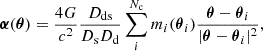
For our lens mass modeling, we used the full-depth combined mosaics of all the data in the five HST and six JWST filters listed in Table 3 of Ertl et al. (2025). These mosaics were produced according to the techniques first described by Koekemoer et al. (2011), updated for the JWST pipeline, with further details about these data presented in Pierel et al. (2024) and Acebron et al. (2025). In Fig. 1, we show a color image of MACS J0138−2155, with the multiple image positions of SN Encore and SN Requiem marked by systems 1 and 2, respectively, along with additional multiple-image systems.
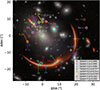 |
Fig. 1. MACS J0138−2155 as observed through HST and JWST with the following combinations of filters for the color image: F105W+F115W+F125W (blue), F150W+F160W+F200W (green), and F277W+F356W+F444W (red). The positions of the “gold” multiple-image systems are shown with circles. SN Encore is System 1, and SN Requiem is System 2. The foreground (fg) and background (bg) galaxies are marked by cyan diamonds. The dashed squares identify some of the freely optimized cluster members in the lens model, i.e., not constrained by the scaling relations for the cluster members (gray for the ZITRIN-ANALYTIC lens model, maroon for the LENSTOOL I, and that labeled with IDphot = 116 for the GLEE and ZITRIN-ANALYTIC models). The three jellyfish galaxies are labeled with light-green crosses as JF-1, JF-2, and JF-3. |
2.2. JWST and MUSE spectroscopy
Supernova Encore and its host galaxy were observed with JWST NIRSpec integral field unit (IFU) for one of the multiple images, namely, 1a and 3a, marked in Fig. 1 (Proposal ID 2345, PI: Newman). With the spectra taken at two epochs, Dhawan et al. (2024) showed that SN Encore, at zs = 1.949, is a Type Ia SN similar to local Type Ia SNe in terms of its spectral features, despite its high redshift.
MACS J0138−2155 was also observed at the Very Large Telescope of the European Southern Observatory using the integral-field spectrograph Multi Unit Spectroscopic Explorer (MUSE; Bacon et al. 2010) through two programs. Program ID 0103.A-0777 (September 2019, PI: Edge) targeted the central ∼1′×1′ field of view (FoV) of the galaxy cluster for nearly 1 hour. Upon the discovery of SN Encore, our team acquired additionally 2.9 hours of observations with the MUSE IFU in December 2023 (Program ID 110.23PS, PI: Suyu). The data from both programs were reduced and analyzed by Granata et al. (2025), who measured 107 reliable spectroscopic redshifts of galaxies in the cluster FoV, including lensed background galaxies.
3. Data products
Building a mass model requires the identification of (1) galaxies that are members of the cluster, (2) line-of-sight (LOS) galaxies that are not part of the cluster but are sufficiently massive to produce significant lensing effects, and (3) background sources that are strongly lensed into multiple images by the foreground cluster and LOS galaxies. Spectroscopic redshifts are also needed for accurate mass models. We summarize the work of Granata et al. (2025) and Ertl et al. (2025) to obtain the ingredients (1) and (2) in Sects. 3.1 and 3.2. We describe our process of defining the sample of multiple images in Sect. 3.3, which provides crucial constraints on the lens mass models.
3.1. Galaxy cluster members
Through the spectroscopic analysis in Granata et al. (2025) and the photometric analysis in Ertl et al. (2025) of galaxies in the cluster FoV, we identified 84 galaxy cluster members, including 50 that are spectroscopically confirmed (providing a cluster redshift value of zd = 0.336). Three of the cluster members are jellyfish galaxies (e.g., Ebeling et al. 2014; Poggianti et al. 2025; Gibson et al. 2025), which are highlighted in light green in Fig. 1 and labeled as JF-1, JF-2, and JF-3. Granata et al. (2025) measured the stellar velocity dispersions for 14 early-type cluster members, which have sufficiently high spectral signal-to-noise ratio, including the brightest cluster galaxy (BCG). These velocity dispersion measurements can then be used to calibrate the Faber-Jackson relation for the cluster members, relating their observed magnitudes to velocity dispersions (and thus total masses). The photometric and velocity-dispersion catalogs of the cluster members are released by Ertl et al. (2025) and Granata et al. (2025), respectively.
3.2. Significant line-of-sight galaxies
Two LOS galaxies, both with spectroscopic redshift measurements from Granata et al. (2025), were explicitly included in the lens mass models. One is a foreground galaxy, labeled as ‘fg’ hereafter, located angularly close to the southern giant arc with (RA, Dec) =  and a redshift of zfg = 0.309. The other is a massive background galaxy, labeled as ‘bg’ hereafter, about 8″ northwest of the BCG at (RA, Dec) =
  and zbg = 0.371. These two objects are marked in Fig. 1.
3.3. Strongly lensed multiple images
Accurate identifications of multiple images are crucial, since wrong identifications introduce biases in the lens mass models. All modeling teams collectively identified the multiple-image systems to ensure both robustness and completeness, given the existing data. We had a two-step procedure: (1) we proposed and reached consensus on the positions of the secure multiple-image systems, and (2) we determined the associated uncertainties for these secure multiple-image systems.
For step (1), we first distributed the HST and JWST images as well as the photometric and spectroscopic catalogs to all the modeling teams. By building preliminary mass models using these data, each team proposed candidates for strongly lensed systems by marking the candidate positions of multiple images that belong to the same system (of the same background source position). In total, the teams collectively proposed approximately 36 candidate systems with a few more candidate systems whose multiple images overlap partly with some of those in the 36 systems. To determine whether a candidate system is robust, we proceeded by voting. Each team voted on every candidate system to indicate whether it thinks the candidate is a secure strongly lensed system. If a team considered a candidate system secure, it then voted on the proposed positions of that system’s multiple images (various teams sometimes proposed slightly different positions for the same candidate-lensed image, and in the voting round, each team voted for one among the proposals). At the time of voting, there were eight independent modeling teams (two of the teams later merged into a single team). Therefore, the maximum number of positive votes a candidate lensed-image position could have was eight, since each team cast one vote.
We defined the following criteria for “gold” and “silver” multiple images, where we consider “gold” as secure and “silver” as likely. For a multiple image and its proposed position to be classified as “gold”, it required seven or eight votes in total and had to belong to a multiple-image system with at least one spectroscopically confirmed multiple image. For a multiple image to be classified as “silver”, it needed to have six to eight votes, without requiring spectroscopic redshift.
Based on the votes, we identified eight gold systems with a total of 23 multiple images, as shown in Fig. 1. We refer to Ertl et al. (2025) for more details about these gold systems. We further identified one silver system corresponding to the spectroscopic ID 1755 (Granata et al. 2025), with a “likely” rather than “secure” redshift measurement from two blended background sources. The silver system has three multiple images, and we refer to Appendix A for more details.
After establishing the multiple image positions of the gold and silver systems, we proceeded to step (2) to estimate their positional uncertainties. The teams agreed to adopt elliptical uncertainties based on the shape of the observed lensed images. The uncertainties typically extend ∼1−3 pixels, in either the JWST or MUSE data, depending on which dataset the lensed system is detected in. The positions of the spatially extended and highly magnified multiple images (e.g., multiple images 3a and 3b) are harder to pinpoint and thus have larger uncertainties (in terms of the number of pixels) compared to those of point-like multiple images such as SN Encore (images 1a and 1b).
In summary, the 23 gold multiple-image positions from the eight systems are listed in Table 4 of Ertl et al. (2025) and shown in Fig. 1. The three multiple images of the single silver system are presented in Table A.1 and Fig. A.1. The lensed background sources span a redshift range between 0.767 to 3.420.
4. Lens mass models
In this section, we summarize the seven modeling approaches using six different software with the same data as input. The modeling approaches are divided into two generic categories, parametric and free-form total mass distributions. The five parametric models from four different software are presented in Sect. 4.1 to Sect. 4.5, and the two hybrid free-form models used in this work are described in Sects. 4.6 and 4.7. We summarize in Table 1 the requirements and capabilities of each software. All can model single-plane lenses with circular positional uncertainties for the multiple images. This setup consequently forms a baseline model for direct comparison of the software and approaches. All models adopted a flat ΛCDM cosmology1 with H0 = 70 km s−1 Mpc−1 and Ωm = 1 − ΩΛ = 0.3 for predicting the multiple image positions, magnifications, and time delays, unless otherwise stated.
Summary of modeling software.
The seven modeling teams were each invited to build two models: (1) a baseline model to facilitate direct comparison between different models, and, optionally, (2) their ultimate model, representing the team’s most suitable mass model for cosmographic inference with SN Encore. For the baseline model, all the mass components (cluster-scale halos, sub-halos, and LOS galaxies) were placed at the cluster redshift of zd = 0.336, and the positional uncertainties were assumed to be circular. The size of the circular uncertainty (σcirc) is the geometric mean of the semimajor (σmajor) and semiminor (σminor) axes of the elliptical uncertainty tabulated in Table 4 of Ertl et al. (2025) and in Table A.1, i.e.,  . In the end, six of the seven teams used their baseline model as their ultimate model. Only the GLEE team built an ultimate model in addition to their baseline model.
4.1. Parametric models.
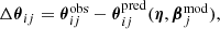
In parametric models, the cluster total mass distribution is often separated into multiple mass components (such as cluster-scale DM halos and galaxies) with each parameterized by a functional form with several parameters. Depending on the parametric model presented in this work, the cluster-scale mass component of MACS J0138−2155 (mainly in the form of DM) is parameterized with one or two mass distributions where the mass density profile was chosen by each team. The mass density profile of individual cluster members is a dual pseudo-isothermal elliptical (dPIE) mass distribution – a truncated isothermal profile (e.g., Elíasdóttir et al. 2007; Suyu & Halkola 2010) with velocity dispersion, σv, i, and truncation radius, rcut, i, as free parameters for the ith cluster member (centroids, axis ratios, and position angles were either varied or fixed to those of the galaxy light distribution, as specified in each mass model’s subsection). Some teams adopted circular (instead of elliptical) convergence profiles for the galaxies in their models, and we use the same nomenclature of dPIE to refer to the mass profiles of the galaxies, irrespective of their ellipticity. Scaling relations between the cluster members’ total masses, Mtot, i ∝ σv, i2rcut, i, and their associated luminosity, Li, enable significant reduction in the number of free parameters. Specifically, the following two scaling relations are generally adopted:
 (1)
(1)
where Lref refers to the reference luminosity of a galaxy at the cluster redshift. The quantities  and
and  were optimized in the lens modeling, and α and β represent the slopes of these scaling relations, respectively. The slope of the total mass-to-light ratio was then obtained as β + 2α − 1. The values chosen for the two slopes then determine whether the cluster members have total mass-to-light ratios that are constant or that increase with their luminosity.
4.2. Free-form and hybrid models.
In contrast to parametric methods, where the mass distribution of the lens is constructed as a sum of analytic halos, whose positions and properties are usually guided by the visible components, the free-form method models the lens by dividing the lens plane into Nc small cells without such informed priors. The deflection field α(θ) is evaluated at the position θ by summing the contributions from all Nc cells as follows:
 (2)
(2)
where mi(θi) is the mass of the ith cell at θi.
The quantity mi(θi) is obtained by minimizing the distance between the model-predicted and observed positions of multiple images. Since the number of free parameters, Nc, exceeds the number of observables, the lens model cannot uniquely be determined. To overcome this degeneracy, regularization schemes, such as entropy, can be applied.
Hybrid models introduce an extra layer of flexibility by incorporating analytic halos, similar to those used in the parametric methods. This hybrid approach is particularly useful when the lensing data are too sparse or when a sharp variation in the deflection field is required, which cannot be adequately represented by free-form mass cells alone.
4.3. Model optimization and statistical estimators.
The values of all the model parameters, η, were varied to fit the observables, which are the 23 multiple image positions of the eight background source positions for the gold sample. Specifically, the posterior probability distribution of the model parameters, P(η|data), was either optimized or sampled, where, through the Bayes theorem,
 (3)
(3)
The likelihood, P(data|η), of the multiple image positions, given a set of model parameters η, is
 (4)
(4)
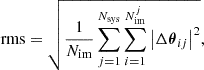
where A is a normalization constant. The χim2 function is given by
 (5)
(5)
where Nsys = 8 is the number of gold systems,  is the number of multiple images of the jth system, and
 (6)
(6)
with  as the observed position of the ith lensed image of system j,
  as the corresponding model-predicted image position,
  as the modeled source position of system j, and σij as the positional uncertainty of the ith image of system j. The above expression is for the case when circular positional uncertainties are considered, and we refer to Ertl et al. (2025) for the expression of elliptical uncertainties. The prior P(η) is based on information from other datasets, such as kinematic measurements of member galaxies in the cluster.
The rms separation between the observed and model-predicted positions of the multiple images is a quantity widely used to assess the goodness of a given lens model. It is expressed as
 (7)
(7)
with Nim = 23 in this paper.
Depending on the complexity of the parametric models, they can have several to dozens of variable parameters. The number of degrees of freedom, Nd.o.f., is computed as
 (8)
(8)
where Nparam = 2 × Nsys + Nmass param. The first term is for the source position parameters, and the second term is for the lens mass-distribution parameters. Besides using the values of χim2 or of the rms to quantify the goodness of a given model, we also compared the values of the Bayesian information criterion (BIC; Schwarz 1978). Even though all the lens models included the same number of multiple images and observables, the BIC is particularly relevant when comparing different total mass parameterizations, with a different number of free parameters. It can be defined as
 (9)
(9)
where  are the maximum-likelihood parameter values. Therefore, up to an (irrelevant) additive constant, the BIC is
 (10)
(10)
where χim, min2 is the minimum χim2 value. For the MrMARTIAN model (see Sect. 4.6), the BIC was computed using the effective number of free parameters for Nparam to account for the effect of regularization, as detailed in Sect. 4.6.
When Nd.o.f. > 0, a good-fitting model has Nd.o.f. ∼ χim, min2. However, mass models might not capture the full complexity of the cluster mass distribution and reproduce the observed image positions within the observational uncertainties, in which case χim, min2 could be substantially larger than Nd.o.f.. In these cases, the model-parameter uncertainties estimated by, for example, MCMC, would be underestimated given the artificially large changes in the likelihood due to the misfit to the observed data. One practical way to mitigate this and obtain realistic model parameter uncertainties is to boost the positional uncertainties of the multiple images such that Nd.o.f. ∼ χim, boost2, where χim, boost2 is the χ2 obtained with the boosted positional uncertainty. For each mass model, we specified the boost factor (1 when no boosting was required to fit to the observed image positions). This boosting applied only to mass-model parameter estimates and predictions. For comparing and weighting the different models, the original χim, min2 was used.
4.4. Overview.
We provide an overview of the setups of the seven lens modeling approaches in Table B.1. For the details of each model, we describe them in the following subsections.
4.1. GLAFIC (M.O., N.F., B.F., S.N., Y.F.)
GLAFIC (Oguri 2010, 2021) is a software for parametric strong lens mass modeling. We modeled MACS J0138−2155 assuming a single lens plane and using only the positions of the multiple images as observables. Since GLAFIC cannot handle elliptical errors for the multiple images positions, circularized errors were adopted for the multiple-image positions.
In the baseline model, we assumed a halo component modeled by an elliptical Navarro-Frenk-White (NFW) mass density profile (Navarro et al. 1997), and a BCG component modeled by an elliptical Hernquist mass density profile (Hernquist 1990). Their lensing properties were calculated by adopting the fast approximation proposed by Oguri (2021). For the NFW component, the mass, centroid position, ellipticity, position angle, and concentration were included as free parameters. The centroid position of the Hernquist component was fixed to the observed position of the BCG, and the mass, ellipticity, position angle, and scale radius were included as parameters. We adopted Gaussian priors for the ellipticity (0.4254 ± 0.05), the position angle (43.59 ± 5.0 deg), and the scale radius ( ), based on the observed light profile of the BCG from Ertl et al. (2025). The lensing effect of most of the other cluster member galaxies was included assuming the dPIE profile using the scaling relation of the velocity dispersion and truncation radius with α = 0.25 and β = 0.5 in Eq. (1), where Li is the luminosity of each galaxy derived from the F115W-band magnitude, and the normalizations of these two scaling relations are free parameters. The galaxies fg and JF-1 were modeled separately, assuming circular dPIE mass density profiles, and their velocity dispersions and truncation radii were free parameters. We also included an external shear in our mass modeling. The number of model parameters is 15, excluding those with informative priors. The best-fitting model has χim2 = 10.8 with 15 degrees of freedom, and the rms of the difference of image positions between the observation and the model prediction is
  .
.
In addition to the baseline model, the mass model using the gold plus silver multiple image sample was constructed. We adopted a Gaussian prior of 2.0 ± 0.5 for the source redshift of the silver multiple-image system. In addition, the member galaxy at (RA, Dec) =  , which affects the multiple images of the silver sample significantly (see Fig. A.1), was modeled separately with a dPIE mass density profile with its ellipticity and position angle fixed to observed values from the light distribution and the velocity dispersion and the truncation radius as free parameters. Thus, the number of model parameters increased to 17, excluding those with informative priors. The best-fitting model has χim2 = 13.9, and a positional rms of
  . The posterior of the source redshift of the silver multiple-image system was dominated by the prior.
The errors of the model parameters were estimated with the MCMC method with a total number of steps of 28871 and 15194 for the baseline and gold plus silver models, respectively. A subsample of 3000 random realizations was used to estimate the distribution of the model-predicted time delays and magnifications for SN Encore and SN Requiem. No rescaling factor was introduced for the positional uncertainty of the multiple images. In our models, 100% of these samples predict five (or more) multiple images both for Encore and Requiem. We note that the baseline model based on only the gold multiple image sample is used for comparison with all the other models in the subsequent analysis, and the results of the gold plus silver images are presented instead in Appendix C.
4.2. GLEE (S.E., S.H.S., S.S., G.B.C., G.G., C.G.)
We built seven different lens mass models with GLEE (Suyu & Halkola 2010; Suyu et al. 2012) with gold images as constraints, exploring a range of DM halo profiles, the presence of a mass sheet, the differences between multiplane versus single-plane modeling, and the impact of having elliptical versus circular BCG. Two of the seven GLEE models are single-lens plane at zd = 0.336, with one adopting elliptical positional uncertainties, and the other one adopting circular positional uncertainties; the latter is the baseline model. The other five GLEE models employed multi-lens planes for the foreground, cluster, and background deflectors, with elliptical positional uncertainties on the multiple images. We refer to Ertl et al. (2025) for details on the GLEE models and summarize here the key aspects and results for the model comparison.
Our GLEE mass models included two DM halos, a primary one centered close to the BCG and a perturbative one that is diffuse with a large core, located ∼30″ southwest of the BCG. In addition, we included the 84 cluster galaxy members and the two LOS galaxies as truncated isothermal profiles into the mass model. We used the Faber-Jackson relation from Granata et al. (2025) to relate the Einstein radii and truncation radii of the cluster members to each other, except for the BCG and the galaxy (IDphot = 116 at (RA, Dec) =  ; Ertl et al. 2025) that is ∼2″ north of the multiple image 4.3a (see Fig. 1), whose Einstein and truncation radii were allowed to vary independently of the scaling relation, given their significant effect on the prediction of the multiple image positions. The three jellyfish galaxies were also not modeled within the scaling relation since the relation applies to early-type galaxies and not jellyfish galaxies. Our reference cluster galaxy for the scaling relations is that with IDphot = 115 in Ertl et al. (2025) with mF160W, ID115 = 17.99. By calibrating the Faber-Jackson relation using the 13 cluster members with velocity dispersion measurements (excluding the BCG), we used the measured value α = 0.25 and a prior on
  of 206 ± 25 km s−1 for the reference galaxy LID115 (Granata et al. 2025) with β = 0.7. We refer to Ertl et al. (2025) for the kinematic priors on the parameters of galaxies not included in the scaling relations.
For each of the seven GLEE models, we ran MCMC chains of 2 × 10⁶ steps. After exploring four different cluster DM halo profiles for the primary lens – including one model allowing a mass sheet at the cluster redshift – we find that cored isothermal DM profiles fit the gold sample of observed multiple image positions well, with a reduced χim2 ∼ 1. This includes our baseline model. Therefore, we do not need to boost the positional uncertainties to quantify our mass-model parameter uncertainties.
We combined four of our five multi-lens plane mass models, which fit well to the observed image positions and have remarkably consistent results, to form our ultimate lens model. We also obtained the baseline model from single lens-plane modeling, for direct model comparison. We find that the baseline model provides a good approximation for our ultimate model. For the predictions of the multiple image positions, magnifications and time delays of SN Encore and Requiem, we thinned the MCMC chains by a factor of 1000. Therefore, the GLEE ultimate model has 8000 samples, and the GLEE baseline model has 2000 samples.
The number of free mass parameters (without informative priors)2 in the GLEE baseline model is 22. From our optimization, we obtain the most-probable χim2 of 7.3, which we approximate3 as χim, min2, with an rms value of 0.24″. We refer to Table 5 of Ertl et al. (2025) for a detailed breakdown of the χim, min2 and rms for the individual gold image systems. While the first four images of SN Encore (images 1a–1d) and SN Requiem (images 2a–2d) were predicted 100% of the time by the mass models in the MCMC chains, images 1e and 2e were only predicted a fraction of the time4, as listed in Tables E.1 and E.2. Images 1d, 1e, 2d, and 2e are predicted to appear in the future.
4.3. LENSTOOL I (P.K.)
The LENSTOOL I model made use of the well-tested LENSTOOL software (Kneib et al. 1993, 1996; Jullo et al. 2007; Jullo & Kneib 2009), adhering to the general methodology followed in Kamieneski et al. (2024a,b) (see also Pascale et al. 2025). Only a baseline model was contributed in this analysis. The MACS J0138−2155 cluster was modeled under the assumption of a single lens plane at zd = 0.336, consisting of an underlying DM halo parameterized as a non-truncated dPIE. An ensemble of 80 cluster member galaxies (out of a total of 84) were included as small-scale, truncated dPIE mass components held at z = 0.336, with small core radii values fixed to 0.15 kpc, and each with their ellipticities and position angles fixed to the morphological fitting by Ertl et al. (2025). Together, they were scaled in velocity dispersion based on their measured luminosities in the F200W band, with α = 0.25 while their truncation radii were scaled with β = 0.5 (which yields a constant total mass-to-light ratio). The normalizations of these relations were optimized as free parameters. Also, the background LOS galaxy, bg, was included in the scaling relations, as it is not in very close proximity to any arcs of the gold image families.
The four cluster members excluded from these scaling relations were instead independently optimized as singular isothermal sphere (SIS) or singular isothermal ellipsoid (SIE) profiles (Kormann et al. 1994), due to a need for greater flexibility in the model (typically as a result of close proximity to one of the gold images). The first of these is at (RA, Dec) =  , optimized as an SIS with fixed centroid (chosen given its proximity to the radial arc of System 3; see the maroon square in Fig. 1). The three other members are apparent jellyfish galaxies requiring some extra care. Specifically, the jellyfish galaxies JF-1 and JF-3 were optimized as an SIS profile (again with fixed centroid). The jellyfish galaxy JF-2 was instead parameterized as an SIE profile (with free parameters of velocity dispersion, ellipticity, and position angle).
The fg near the multiple image 3b was independently modeled as an SIS with its centroid and velocity dispersion as free parameters. Finally, an external shear component was included in the model, primarily to account for deficiencies in this parameterization. In total, the model included 20 free parameters. Uniform priors were used for all the parameters, except for (i) the centroid of the primary cluster halo component, (ii) the centroid of the LOS fg, and (iii) the truncation radius of the cluster halo. These parameters were optimized with Gaussian priors instead, with σ = 2.0″, 0.5″, and 100 kpc (centered at 1000 kpc), respectively.
The baseline model was constrained using only the observed positions of the gold set of multiple images and optimized on the image plane. The multiple image positions in the highest-likelihood model were recovered with an image-plane rms offset of  . The positional uncertainties were then uniformly rescaled by a factor of 2.2 to ensure a reduced χim2 < 2, and a χim2 of 19.2 is achieved for 10 degrees of freedom.
The posteriors were estimated from 300 realizations randomly drawn from the final MCMC chain, which contained 10 000 iterations after burn-in. In our baseline model, 100% of these samples predict a fourth image of SN Encore (1d), but only ∼4% of the realizations predict a fifth image (1e). For SN Requiem, ∼16% of iterations predict the fourth image (2d). None of the realizations predict a fifth image (2e).
After the lens modeling unblinding, an alternative model was tested to examine the cause of the large uncertainties for the time delays between different pairs of images (see Sect. 5.2). We found significant covariance between the free parameters for JF-2 (namely, ellipticity and velocity dispersion) and the time delays, perhaps due to its proximity to the BCG. For the alternative model, JF-2 was instead parameterized as an SIS potential, thus with only one free parameter instead of three. This resulted in minimal change to the χim2 value, but relative time-delay uncertainties that were much more consistent with those from the other lens models (see Appendix D).
4.4. LENSTOOL II (A.A., P.B., P.R.)
A second team also used the parametric LENSTOOL software (Jullo et al. 2007) to model the total mass distribution of MACS J0138−2155 following the methodology outlined by, for example, Caminha et al. (2019), Bergamini et al. (2023), Acebron et al. (2022). The strong-lensing analysis is detailed in Acebron et al. (2025), where several total mass models were explored to assess the impact of systematic uncertainties on the model-predicted positions, magnifications, and time delays of the SN Requiem and SN Encore multiple-image systems. We summarize here the characteristics of our best-fitting lens model, labeled as reference in Acebron et al. (2025), and presented to this comparison challenge as our baseline model. The six lens models explored by Acebron et al. (2025) enable one to assess the impact of modeling choices on the model-predicted time delays of both SNe systems. We found that the different mass parameterizations yield model-predicted values of their magnifications and time delays that are consistent within the 1σ uncertainties, provided that fg is taken into account.
The total mass distribution of the lens was modeled with a single cluster-scale halo, parameterized with a non-truncated elliptical dPIE mass density profile and an external shear component. The sub-halo component, as well as the three jellyfish members and the two LOS galaxies, were described instead with circular, truncated dPIE mass density profiles, with vanishing cores. The values of the normalization and slope of the kinematic scaling relation were anchored on the calibrated Faber-Jackson relation including the BCG (see Acebron et al. 2025, using the measurements from Granata et al. 2025). Specifically, we adopted a Gaussian distribution centered on the measured value of 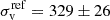 km s−1 (associated with the BCG with mF160W = 15.30), as a prior for the normalization of the kinematic scaling relation. Its slope was instead fixed to the best-fit value of α = 0.21, while the value of β is inferred to be equal to 0.71. Thus, the 81 cluster member galaxies were scaled with total mass-to-light ratios that increase with their F160W luminosities, as M/L ∝ L0.2, consistent with the observed tilt of the Fundamental Plane. The three jellyfish member galaxies and the two LOS galaxies were modeled outside of the scaling relations, with their mass parameters free to vary. The values of all the model parameters except that of the scaling relation normalization,
  , were optimized within large flat priors (see Table 2 in Acebron et al. 2025).
Our baseline model of the MACS J0138−2155 total mass distribution includes 20 free mass parameters and reproduces the observed positions of the multiple images with a rms offset of  . The final model was obtained after rescaling the multiple images positional uncertainty by a factor of 1.5. The median values and the associated 1σ uncertainties of the model-predicted quantities were obtained from 1000 different models randomly extracted from the MCMC chain, with a total number of 5 × 10⁵ samples, excluding the burn-in phase. Our baseline model predicts the reappearance of both SN Encore and SN Requiem in the future, with two and one additional multiple image(s), respectively, in the radial arc of MACS J0138−2155. We note that our model predicts the fifth and central multiple image of SN Encore, 1e, in only ∼15% of the chains.
4.5. ZITRIN-ANALYTIC (A.K.M., A.Z.)
This lens model was constructed using a revised version of the parametric approach described in Zitrin et al. (2015), which is sometimes also referred to as “Zitrin-analytic”. The underlying modeling approach is similar to that from other parametric lens modeling techniques and has been successfully applied to many other galaxy clusters (e.g., Furtak et al. 2023, 2024; Meena et al. 2023; Pascale et al. 2022, 2025). The model primarily contains two parametric mass components as isothermal halos to describe the DM, and dPIE for galaxy-scale components. The method calculates the various lensing quantities directly at the positions of multiple images.
For the MACS J0138−2155 baseline model, we used two DM halos placed around the BCG and bg positions, and the DM positions were optimized in the minimization. Each dark-matter halo thus had six free parameters: the velocity dispersion, core radius, ellipticity, position angle, and the two-dimensional position. We also left free to vary the core radius, ellipticity, and position angle of the BCG and of bg. The rest of the cluster galaxies were assumed to be circular and modeled using the scaling relation given by Eq. (1), but with a core. For the scaling relations, we used (α, β, γ) = (0.25, 0.50, 0.50) where γ represents a similar scaling for the core radius. We used a core size value of  kpc for the reference (roughly ∼L*) galaxy, whereas σref and
  were optimized in the minimization. In our model, which does not include an external shear, we also left free to vary the velocity dispersions of four of the circular cluster galaxies with (RA, Dec) =
  ,
,  ,
,  , and
, and  . As illustrated with the dashed gray squares in Fig. 1, these four galaxies are located west of the BCG, and their model parameters were free to vary to improve the reproduction of nearby images. We obtained a total of 24 free parameters.
The lens model was optimized on the source plane using an MCMC sampling (where the χ2 is defined on the source plane based on the separation of the mapped source positions corresponding to the observed image positions, instead of χim2 in Eq. 5)5, with a couple of hundred thousand steps after the burn-in phase. For more details about the modeling scheme and minimization procedure, we refer to Furtak et al. (2023). With the above setup, we got (χim2, Nd.o.f., image rms) = (143.2, 8,  ), where we boosted the nominal positional uncertainties as described in Sect. 3.3 by a factor of 3 (such that the output χim2 was 15.91 in the minimization). To generate the errors, we drew 1000 random points from the final MCMC chain. In our sample, 90% and 94% of solutions led to the formation of a fifth image (1e and 2e) close to the center of the lens cluster for Encore and Requiem, respectively.
4.6. MrMARTIAN (S.C., M.J.J.)
MrMARTIAN stands for Multi-resolution MAximum-entropy Reconstruction Technique Integrating Analytic Node and augments the free-form capability of MARS (Cha & Jee 2022, 2023; Cha et al. 2024) by incorporating analytic nodes. This hybrid approach allows us to model lens features smaller than the grid size using analytic halo mass-density profiles where required by the data, while efficiently representing larger scales with a flexible grid regularized by entropy (Cha & Jee 2026). The grid component of MrMARTIAN differs from that of MARS in that the grid size is nonuniform across the field, enabling multi-resolution capability by assigning higher-resolution grids to the regions where the mass density changes more rapidly. To predict the lens properties at any arbitrary location, we summed the contributions from both the analytic nodes and the multi-resolution grid.
In our lens modeling of MACS J0138−2155, we used only one truncated pseudo-elliptical NFW node consisting of seven free parameters: x, y coordinates, concentration, scale radius, ellipticity, position angle, and truncation radius. We did not incorporate any observed photometric information as informed priors; only the BCG position was used to set the initial location of the node center. Together with the multi-resolution grid, which consists of three resolution levels ( /pix,
/pix,  /pix, and
  /pix), the total number of free parameters amounts to 2225. While this is higher than for the parametric methods, the effective number of free parameters would be lower than 2225, as the regularization term prevents each parameter from varying independently. To quantify the impact of the regularization, we calculated the effective number of free parameters using two different methods. The resulting values are 64.2 and 11.9, based on Moody (1991) and Spiegelhalter et al. (2002), respectively. The rms of the predicted multiple image positions is
  , and the offset between the BCG and the halo position from our lens model is
  . To estimate the posterior distributions, we generated 200 realizations from randomly selected initial conditions6. All of our realizations predicted the fourth and fifth images of both SN Encore and SN Requiem. Following the submission of the blinded model by the MrMARTIAN team, a minor issue was discovered involving the fixed prior intervals for the position angles in the analytic halos. While the best-fit results remained unaffected, the parameter uncertainties were overestimated. The postblind model offers more reliable uncertainty estimates.
We also constructed a lens model using the gold plus silver systems. To represent a compact halo located south of the silver images (see Fig. A.1), we included an additional analytic node, which is also modeled with seven free parameters. The redshift of the silver multiple-image system was treated as a free parameter in the lens modeling, with a flat prior range of [0.436, 15]. The total number of free parameters amounts to 2233, and the rms of the predicted multiple image positions is  . The model-predicted redshift of the silver system is
 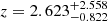 . Similar to the model using gold samples, all of our realizations predict the fourth and fifth images of both SN Encore and SN Requiem. We refer to Appendices A and C for more details.
4.7. WSLAP+ (J.M.D.)
This code was first described in Diego et al. (2005) and later expanded in Diego et al. (2007) to include weak lensing measurements as additional constraints. A further development was presented in Sendra et al. (2014) where the code migrated from its native free-form nature to a hybrid type of modeling, with prominent member galaxies added to the lens model using a mass distribution that matches the observed light distribution.
WSLAP+ placed Gaussians in a predetermined grid of positions in the lens plane. The mass of each Gaussian was optimized by the algorithm. A contribution from member galaxies was also precomputed by adopting a fiducial mass for them, which was later optimized. A joint solution for the masses of the Gaussians, renormalization of the mass of the member galaxies, and unknown position of the lensed galaxies in the source plane was obtained by solving a system of linear equations:
 (11)
(11)
where Φ is an array containing the observed positions of the multiple images, Γ is a known matrix, and X is the vector with all the unknowns: total masses in the Gaussian decomposition (M), multiplicative factors for the fiducial mass of the member galaxies (C), and source positions (βx and βy). The solution was obtained using a quadratic programming optimization algorithm with the constraint Xi > 0, where i denotes the ith component of vector X7.
For the particular case of MACS J0138−2155, we used 252 Gaussians with varying widths, where smaller Gaussians were placed near the BCG, thus increasing the resolution. We also superimposed additional layers of mass components associated with the luminous galaxies, where each layer has one single mass-to-light scaling parameter that is free to scale the observed light to mass. The luminous galaxies expected to have different mass-to-light scaling were thus placed in different layers. For MACS J0138−2155, we adopted four layers (i.e., four additional free parameters) for the total mass associated with the member galaxies, which was assumed to trace the observed light in the F356W filter. Layer 1 contained the BCG, layer 2, all the remaining non-jellyfish member galaxies, layer 3, the jellyfish galaxies, and layer 4, fg and bg. All galaxies were assumed to be at the same redshift. Since WSLAP+ needed to optimize also for the unknown source coordinates (βx and βy) of the eight gold systems, the total number of free parameters amounted to Nparam = 252 + 4 + 2 × 8 = 272. The derived lens model has an rms varying between  arcsec for some of the positions of the SN Requiem and up to
  arcsec for system 4. Considering the full sample of multiple images, the rms is
  . The χim2 value from Eq. (5) is very high, 2136.5, as reported in Table 2. This high value is mostly due to the relatively large offset between some of the observed and predicted positions of the SNe and host galaxy. More precisely, 99.898% of the χim2 (that is, 2134.32 out of 2136.5) comes from the constraints on the host galaxy. This is not unusual in WSLAP+ models that sometimes predict larger offsets (along the arcs) in images close to forming Einstein rings, as it is the case for the host galaxy. Nine separate modeling runs were used to estimate the uncertainties of the predicted image positions, magnifications and time delays of the SNe by taking the mean and standard deviation of the results from the nine runs. All models predict five multiple images for SN Encore and SN Requiem. After unblinding, it was discovered that the computation of the time delay (from the deflection field and potential) was affected by incorrectly rescaling the lensing potential from the fiducial redshift (zs = 3) to the redshift of the two SNe. Hence, we labeled these corrected predictions for the time delay as “postblind”, although both the fiducial deflection field and potential were computed before unblinding.
Summary of the characteristics of the seven lens models of MACS J0138−2155.
5. Comparison of the lens mass models
The key characteristics of the best-fitting lens models from each team are summarized in Table 2. For each of them, we report the number of free model parameters, degrees of freedom, as well as the values of the statistical estimators introduced in Sect. 4. We compare in Table 2 the baseline models that are constructed by all the seven teams using the same circular positional uncertainties (which enable direct model comparison). Only the GLEE team constructed a separate ultimate model with multiplane lensing and elliptical positional uncertainties; we report the GLEE predictions of SN properties but cannot compare the values of the statistical metrics to the other models given the difference in the data (elliptical versus circular positional uncertainties). For a direct comparison of χim, min2 from the various models, we use the multiple image positional uncertainties for the baseline models without boosting, even though some teams boosted the positional uncertainties to obtain their model parameter constraints and model predictions (see Sect. 4). The goodness of fit to the observables varies across the seven lens models, where four teams obtain a χim, min2 of < 25, with two teams reaching χim, min2 < 11. The corresponding values of the rms vary between  to
to  . We note that the relationship between the χim, min2 and rms is nonlinear, since image positions identified from JWST have uncertainties that are approximately ten times smaller than those from MUSE (see Ertl et al. 2025). The GLEE and the GLAFIC total mass models achieve the lowest values of χim, min2 and the BIC, respectively.
5.1. Surface mass density of the cluster mass distribution
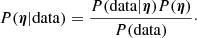
In Fig. 2, we show the best-fit total surface-mass-density profiles of the seven lens models presented in Sect. 4. We find that the profiles are in fairly good agreement, despite the different modeling approaches and assumptions. The agreement is especially noteworthy at projected distances from the BCG between 20 and 70 kpc, where most of our observables are located (marked with vertical lines in the figure). The largest discrepancies arise both at small (≲10 kpc) and large (≳100 kpc) projected distances from the BCG, where only a few multiple images are identified and model extrapolation become relevant. In particular, in the innermost region of MACS J0138−2155, where our models predict the reappearance of multiple images (d and e) of SNe Requiem and Encore, the inferred slope varies considerably between lens models, from relatively cuspy (LENSTOOL I and II) to flat (ZITRIN-ANALYTIC) total surface-mass-density profiles.
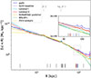 |
Fig. 2. Total average surface-mass-density profiles of MACS J0138−2155 as a function of projected distance from the BCG center for the different best-fit strong-lensing models. The vertical lines (at the bottom of the panel) show the observed positions of the 23 multiple images in the gold sample, where the positions of the multiple images of SN Encore and SN Requiem are highlighted in red and blue, respectively. The vertical gray lines (at the top of the panel) mark the positions of the JF-1, JF-2, and bg galaxies, which contribute significantly to the surface mass density at their locations in some models. The inset shows a zoom-in of the region delimited by the dashed rectangle, where the observed multiple images of the two SNe are located. |
5.2. SN Encore image positions, magnifications and time delays
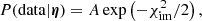
In Fig. 3 and Table E.1, we show the model predictions from the different teams for each of the multiple images of SN Encore, based on the assumed flat ΛCDM cosmology with H0 = 70 km s−1 Mpc−1. We start noticing that the majority of the blindly model-predicted quantities from the different teams are consistent, given the estimated statistical uncertainties. In particular, three parametric models (GLAFIC, GLEE, and LENSTOOL II) can reproduce very well the observed positions of images 1a and 1b (labeled in Fig. 1), and one of the free-form models (WSLAP+) cannot reproduce the same images within their errors. Images 1a and 1b are, respectively, predicted to be magnified with factors ranging from approximately −30 to −20 (the sign is negative since image 1a is a negative-parity lensed image) and from 30 to 40. Image 1b is predicted by most of the models to have a time delay of about −40 days (with a relative error of ≈10%) with respect to image 1a (i.e., Δt1b, 1a ≡ t1b − t1a ∼ −40 days).
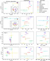 |
Fig. 3. Model predictions for SN Encore’s image positions (left), magnifications (middle), and time delays (right) for a fixed cosmological model (flat ΛCDM with H0 = 70 km s−1 Mpc−1 and Ωm = 0.3 = 1 − ΩΛ). Each row corresponds to one lensed image, as labeled in the top-left corner of each panel in the left column. The coordinate positions are relative to the BCG in arc seconds. The black circle marks the observed image positions of 1a and 1b (left panel in first and second rows, respectively) with the circular radius corresponding to the 1σ positional uncertainty. The insets for the image positions 1a and 1b (left panels) show a zoom-in of the region near the observed image position. The time delays (in days) are relative to image 1a of SN Encore, discovered in November 2023, i.e., Δti, 1a ≡ ti − t1a. |
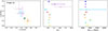 |
Fig. 3. continued. |
All models predict three additional multiple images of SN Encore, although two of them (1c and 1e) are not present in all the iterations of the final chains of the teams. In cases where an image is not predicted in all the iterations of a team’s model, the properties of the predicted image are computed based only on the iterations that have the image predicted. Interestingly, images 1d and 1e are expected to appear in the future, more than 3000 days after image 1a, while image 1c should have appeared about a year before image 1a. Given the long time-delay values of images 1d and 1e, their relative errors can be predicted with statistical uncertainties as low as 2% by some of the models and 1% by the MrMARTIAN model. The predicted image positions of 1d and 1e show scatter among the models due to the presence of nearby jellyfish galaxies JF-1 and JF-2 (see Fig. F.1); the predicted positions of 1d and 1e are thus sensitive to the modeled mass distributions of JF-1 and JF-2, which are currently not well constrained by the existing multiple-image systems. The magnification factors of images 1c, 1d, and 1e are significantly smaller than those of images 1a and 1b, going from slightly more than 10 for image 1c, to approximately −4 for image 1d, to order of unity for image 1e.
5.3. SN Requiem image positions, magnifications and time delays
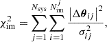
Similarly to Sect. 5.2, we compare here the model predictions from the different teams for each of the multiple images of SN Requiem, as shown in Fig. 4 and Table E.2. The general remarks about the overall consistency of the model-predicted quantities for SN Encore are valid also for SN Requiem. It is confirmed that the same three parametric models (i.e., GLAFIC, GLEE, and LENSTOOL II) and the free-form MrMARTIAN model can reproduce more accurately than the other models the observed positions of images 2a, 2b, and 2c. These three images of SN Requiem are always predicted by all the models, with magnification factors mostly between −40 and −30, 20 and 30, and 10 and 20, respectively. The magnitudes of the magnification values are several times higher than those predicted by the models of Newman et al. (2018a) and Rodney et al. (2021), likely due to the new JWST and MUSE datasets that enable more accurate mass models (see also the discussion in Acebron et al. 2025). The predicted positions of images 2d and 2e show larger scatter, due to the presence of nearby jellyfish galaxies JF-1 and JF-2 (see Appendix F and Fig. F.1).
 |
Fig. 4. Model predictions for SN Requiem’s image positions (left), magnifications (middle), and time delays (right) for a fixed cosmological model (flat ΛCDM with H0 = 70 km s−1 Mpc−1 and Ωm = 0.3 = 1 − ΩΛ), in the same format as Fig. 3. The black circle marks the observed image positions of 2a, 2b, and 2c with the circular radius corresponding to the 1σ positional uncertainty. The time delays (in days) are relative to image 2a of SN Requiem. The measurements of Δt2b, 2a and Δt2c, 2a from Rodney et al. (2021) based on the color curves of the SN Ia template are shown by the vertical line, with the shaded interval marking the 1σ uncertainty. |
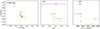 |
Fig. 4. continued. |
The time delays of images 2b and 2c with respect to image 2a were estimated in Rodney et al. (2021) by using color curves of SN Ia templates (see Extended Data Fig. 5 of Rodney et al. 2021 that is based only on SN colors and not on lens mass models). Both values are close to −120 days, with 1σ relative errors of about 25%. These measurements were not used by the teams in their model optimizations. While most of the model-predicted time delays of Δt2c, 2a (with H0 fixed to 70 km s−1 Mpc−1) are consistent with the measured value within 1σ, the model-predicted time delays of Δt2b, 2a are approximately a factor of 2 shorter than the measured ones. This is not particularly concerning, given that the measured delay of SN Requiem is based on only a single epoch of photometry and the assumption that it is of Type Ia, both of which introduce significant uncertainties that may not be fully captured in the Requiem delay measurement. In contrast, SN Encore is spectroscopically classified to be Type Ia and is observed in multiple epochs, leading to reliable time-delay measurement uncertainties for cosmography (Pierel et al. 2024, 2026).
Two additional multiple images of SN Requiem are predicted: image 2d by all teams, image 2e only by some teams. Images 2d and 2e are expected to be less magnified than the other three images, with magnification factors of approximately −3 and 1.5, respectively. Both images have model-predicted time delays of about 4000 days relative to image 1a, so they should be visible in the future.
6. Relation between H0 and time delays
For a given mass model, we can predict the time delays, Δtfc, for fixed cosmological parameters, where Δtfc is a vector with a length equal to the number of multiple images that will have time-delay measurements. From Sect. 4, we obtain from each team the following predicted time delay for a given set of mass-model parameter values η and fixed cosmological parameters:
 (12)
(12)
where the subscript ‘fc’ stands for fixed cosmology, and i denotes the ith sample in the distribution.
The scaled deflection angles depend on the ratios of angular diameter distances for different lens and source redshifts; therefore, they are independent of H0 since H0 cancels in the ratio of distances. However, the ray tracing does depend on non-H0 cosmological parameters such as Ωm for systems with multiple-lens or source redshifts. Therefore, by fixing all cosmological parameters except for H0, the ray tracing and thus the predicted image positions remain invariant. This is true for both single-lens plane and multi-lens plane modeling. In this case, we can simply predict the time delays for a given H0 value using
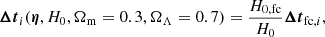 (13)
(13)
where H0, fc = 70 km s−1 Mpc−1.
Armed with Eq. (13), we can derive the constraints on H0 for hypothetical time-delay measurements in a flat ΛCDM cosmology with Ωm = 0.3. Suppose we have hypothetical time-delay measurements of Δtdata with the covariance matrix between the delay measurements denoted by CΔt. The time-delay likelihood of the measurements (Δtdata) given model-predicted delays (Δtmodel) is
![Mathematical equation: $$ \begin{aligned} \begin{aligned} \mathcal{L} _{\Delta t} =&\frac{1}{Z} \exp \bigg [-\frac{1}{2} \left({\boldsymbol{\Delta t}}_{\rm data}-{\boldsymbol{\Delta t}}_{\rm model}\right)^\mathrm{t} C_{\rm \Delta t}^{-1} \\& \left({\boldsymbol{\Delta t}}_{\rm data}-{\boldsymbol{\Delta t}}_{\rm model}\right)\bigg ], \end{aligned} \end{aligned} $$](/articles/aa/full_html/2026/04/aa57235-25/aa57235-25-eq56.gif) (14)
(14)
where t denotes transpose and Z is the normalization constant. We can importance sample the original distribution of time delays Δtfc, i to obtain the resulting H0 constraint as follows. For each sample i in the distribution, we (i) draw a random H0 value, (ii) compute the predicted time-delay Δti via Eq. (13), (iii) compute the likelihood ℒΔt, i of the hypothetical time-delay measurement Δtdata and predicted delay Δti (i.e., Δtmodel = Δti in Eq. (14)), and use this as weight wi for the sample i. The weighted distribution of H0 is then the probability distribution of H0.
For background cosmological models where non-H0 parameters are not the flat ΛCDM model with Ωm = 0.3 = 1 − ΩΛ, then the ray tracing changes in the modeling and the corresponding image position χim2 changes as well. To get cosmological constraints in these cases, we would need to sample the joint image-position and time-delay likelihoods with our mass model and cosmological parameters (see, e.g., Grillo et al. 2024). Since we completed the lens mass modeling before the time-delay measurements of SN Encore as the core experimental design of our blind analysis, we therefore defer such H0 inference in more general cosmological models to future work.
For SN Encore, where images 1a and 1b are clearly visible in our JWST data and image 1c is barely visible, it may be possible to derive two time delays with the existing data. The 1b–1a delay, Δt1b, 1a, will likely be substantially more precise than Δt1c, 1a, given that image 1c is faint. In this case, the cosmological inference will be mostly determined by Δt1b, 1a. We therefore consider here only Δt1b, 1a in order to derive the relation between H0 and the hypothetical time-delay values. This will avoid exploring implausible combinations of Δt1b, 1a and Δt1c, 1a, which we cannot currently foresee since we do not know the time delays, in order to keep our analysis blind.
We considered 10% relative uncertainties on Δt1b, 1a of SN Encore and obtained Fig. 5, which ranges from −60 to −20 days, covering the 1σ range of predictions from five of the seven teams and lying partly within 2σ of the predictions from the remaining two teams. The corresponding H0 values range approximately from 40 to 170 km s−1 Mpc−1 for six of the seven models (except for the LENSTOOL I model that spans to ∼330 km s−1 Mpc−1), with minimum relative errors of about 12% for the 10% relative uncertainties on Δt1b, 1a.
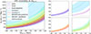 |
Fig. 5. Resulting H0 from different mass models for a range of possible Δt1b, 1a measurements with 10% uncertainty from SN Encore in a flat ΛCDM cosmology with Ωm = 1 − ΩΛ = 0.3. The median values of H0 are shown as solid lines, while the shaded regions indicate the 1σ uncertainty. Left panel: All model predictions overlaid, as indicated in the legend. Right four panels: Subset of the model predictions plotted in the same style as in the left panel, for better visibility. |
In Figs. 6 and 7, we show potential estimates of the value of H0 from hypothetical time-delay measurements of the future multiple images 1d and 2d of, respectively, SNe Encore and Requiem. Given the long (between ≈3000 and ≈4000 days) model-predicted time delays, it might be possible to measure them with a relative uncertainty as low as 1%. A measurement of one of these time delays would result in a H0 measurement with a competitive statistical relative error of ≈2−3%. Interestingly, according to our models, it is likely that the next reappearance of SN Requiem (image 2d) could be detected already at the end of 2025, while that of SN Encore (image 1d) not earlier than mid-2031. Only HST/JWST imaging might be able to reveal these faint and unique transient events.
 |
Fig. 6. Resulting H0 from different mass models for a range of possible Δt1d, 1a measurements from SN Encore in a flat ΛCDM cosmology with Ωm = 1 − ΩΛ = 0.3. The median values of H0 are shown as solid lines, and the shaded regions indicate the 1σ uncertainty. The assumed 1% uncertainty on Δt1d, 1a is achievable given the long time delay of ∼3000 days. |
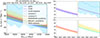 |
Fig. 7. Resulting H0 from different mass models for a range of possible Δt2d, 2a measurements from SN Requiem in a flat ΛCDM cosmology with Ωm = 1 − ΩΛ = 0.3. The median values of H0 are shown as solid lines, and the region delineated by shades indicate the 1σ uncertainty. The relation from the LENSTOOL I model exhibits larger statistical fluctuations since image 2d is predicted in only 16% of the samples for that model (see Table E.2). The assumed 1% uncertainty on Δt2d, 2a is achievable given the long time delay of > 3000 days. |
7. H0 inference from the first SN Encore time-delay measurement
7.1. Time-delay measurement Δt1b, 1a
Pierel et al. (2026) obtained the photometry of SN Encore images 1a and 1b with two different methods, while the photometry of image 1c cannot be robustly determined with existing data. Pierel et al. (2026) measured a time delay of  days using their photometric measurements, SN Ia template light curves from BayesSN (Mandel et al. 2022; Ward et al. 2023; Grayling et al. 2024) and two different fitting methods, GLIMPSE (Hayes et al. 2024, 2026) and SNTD (Pierel & Rodney 2019). The measurement uncertainties account for the effect of microlensing using a suite of microlensing simulations based on four different models of SN Ia progenitors, following the microlensing simulations of Huber et al. (2021). The time-delay uncertainties of ∼9−10% are currently dominated by the photometric precision.
7.2. Combination of lens mass models for cosmography
The independent mass models built by the seven teams using a variety of software allow us to quantify systematic uncertainties arising from lens modeling software and choices. By combining these models to infer H0, our measurement incorporates both statistical and systematic uncertainties associated with cluster mass modeling.
One key aspect in the combination of models is the weighting of the models, since the models have different numbers of parameters and goodness of fit to the observables, especially the multiple image positions. With the wide range of software used, including both parametric and free-form approaches, and the different priors adopted by the teams on some of the model parameters, the number of degrees of freedom is highly nontrivial to compute. The BIC values in Table 2 do not fully account for the subtleties associated with the adopted priors on the parameters. Furthermore, in the case of free-form mass models, the methods for computing the effective number of free parameters for MrMARTIAN can alter the BIC values significantly (as shown in Table 2). Therefore, for inferring H0, we weighted the models based on their maximum likelihood of the observables, which is the product of the likelihood of the observed image positions and the likelihood of the time delay. Given the single time-delay measurement, Δt1b, 1a, the value of the parameter H0 can adjust to each model and yield the same maximum time-delay likelihood. Thus, the weights of each model was determined solely by the maximum likelihood of the observed image positions.
We tabulate in Table 2 the value of the multiple image positions likelihood ℒ in the last column and use these as the weights of the models. We emphasize that the weights of the models were determined before the time delay of SN Encore was measured and before the unblinding of the H0 inference that we present next.
7.3. H0 inference
Using the formalism developed in Sect. 6, we can compute the H0 distribution for each mass model given the measured time-delay distribution of Δt1b, 1a by Pierel et al. (2026). We adopted a prior range on H0 that is uniform between [0, 150] km s−1 Mpc−1, and fix Ωm = 1 − ΩΛ = 0.3. In the top panel of Fig. 8, we show the H0 probability distribution from each of the mass models. In the bottom panel, we show instead the H0 distribution from the combination of the mass models weighted by the likelihood. The inferred value is  km s−1 Mpc−1 (68% CI). Most of the uncertainty on H0 stems from the time-delay uncertainties of ∼9 − 10% and the nonlinear relation between H0 and Δt1b, 1a shown in Fig. 5.
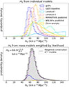 |
Fig. 8. H0 inference from SN Encore using the time-delay measurement Δt1b, 1a by Pierel et al. (2026). Top: Inferred H0 distribution from the mass models of the seven modeling teams via blind analysis, where the mass models and the time delay were kept blind to each other throughout and combined after unblinding without modifications. Bottom: H0 from the combined mass model, weighted by each model’s likelihood. The weights were determined before unblinding (see Table 2). Our |

Our H0 measurement is statistically consistent with previous H0 measurements from SN Refsdal (Kelly et al. 2023; Grillo et al. 2024; Liu & Oguri 2025) and SN H0pe (Pascale et al. 2025), the only other two lensed SNe from which H0 has been inferred, as shown in Fig. 9. Supernova Refsdal is a core-collapse SN (Kelly et al. 2015), whereas SN H0pe is of type Ia (Frye et al. 2024). The measurement of H0 by Kelly et al. (2023) for SN Refsdal and by Pascale et al. (2025) for SN H0pe also combined multiple mass models weighted by observables including the image positions, time delays and magnifications of the lensed SN images. In our case with SN Encore, we currently have only a single time-delay measurement Δt1b, 1a; our weighting by the likelihood of the image positions is thus equivalent to weighting by the likelihood of both the image positions and time delay, as explained in Sect. 7.2. Since magnifications can be affected by microlensing and millilensing, especially in the case of SN Encore with the fg near SN image 1b, we did not incorporate the magnification of the SN Encore images into the weighting of the mass models.
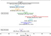 |
Fig. 9. Comparison of H0 measurements from lensed SNe, local distance ladders, and the CMB (Planck Collaboration VI 2020). The H0 values inferred from the lensed SNe shown in the figure assume a flat ΛCDM cosmological model with Ωm = 0.3 = 1 − ΩΛ, except for the measurement by Grillo et al. (2024) from SN Refsdal, which assumes a more general cosmological model with variable matter density, Ωm, spatial curvature, and dark energy equation of state, w. With the current uncertainties, the H0 from SN Encore is statistically consistent with measurements from SN Refsdal (Kelly et al. 2023; Grillo et al. 2024; Liu & Oguri 2025), SN H0pe (Pascale et al. 2025), and the two distance-ladder approaches of the SH0ES (Riess et al. 2022) and CCHP (Freedman et al. 2025) programs, and the CMB. |
Furthermore, our H0 value is also statistically consistent with that of the SH0ES (Riess et al. 2022), CCHP (Freedman et al. 2025) and Planck Collaboration VI (2020) measurements, as shown in Fig. 9. Future observations of SN Encore and Requiem will help significantly reduce our H0 uncertainties for assessing the Hubble tension, which we show next.
8. Predicted reappearance of SN Requiem and SN Encore
Using the model weighting described in Sect. 7.2, we combined the seven models to predict the reappearance of SN Requiem and SN Encore. Specifically, we weighted the predictions in Tables E.1 and E.2 (see also Figs. 6 and 7) by the likelihoods ℒ in Table 2, to obtain the results shown in Fig. 10, assuming a time-delay uncertainty of 1% for each SN. Overlaid on the plots are the measurements of H0 from Riess et al. (2022) and Planck Collaboration VI (2020). As noted in Sect. 6, a detection of the reappearance of either SN will provide a time-delay measurement with ∼1% uncertainty and allow us to distinguish between the SH0ES and Planck H0 values. In particular, if H0 = 73 km s−1 Mpc−1 matching SH0ES, then the four best-fitting mass models (with the lowest χim, min2 values) predict that the next image (2d) of SN Requiem will appear approximately April–December 2026; if H0 = 67 km s−1 Mpc−1, then it is predicted to appear approximately March–November 2027 (based on 1σ uncertainties).
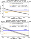 |
Fig. 10. Forecast of the reappearance dates for SN Encore image 1d (top panel) and SN Requiem image 2d (bottom panel). The prediction from the weighted combination of the seven models is shown in black, with shaded 1σ uncertainties, assuming a 1% time-delay uncertainty. The H0 measurements from Planck Collaboration VI (2020) and SH0ES (Riess et al. 2022) with their 1σ uncertainties are overlaid. Given the long time delays of images 1d and 2d, detecting the reappearance of each SN enables time-delay measurements with ∼1% uncertainty and H0 with 2−3% uncertainty. |
Recently, O’Donnell et al. (2025) have predicted the appearance of SN Requiem image 2d to be between January 2027 and November 2028, using their mass model and adopting the H0 value of Planck Collaboration VI (2020). Our prediction for the appearance of image 2d is in the earlier range of the prediction of O’Donnell et al. (2025). We caution against a direct comparison because the datasets used to constrain the cluster mass model are different between ours and that of O’Donnell et al. (2025). In particular, we used 23 multiple images from four distinct background sources, whereas O’Donnell et al. (2025) focused on additional multiple-image systems in the host galaxy of the two SNe and did not include source galaxies at other redshifts. O’Donnell et al. (2025)’s resulting lens model and thus inferred H0 value could be more affected by the mass-sheet degeneracy, as shown in Fig. A.1 of Grillo et al. (2020).
Using the same model weighting approach, we obtained the magnification of the weighted combination of models for SN Encore image 1a as  and image 1b as
  . Since SN Encore is of type Ia, Pierel et al. (2026) determined the absolute magnifications of images 1a and 1b by comparing their observed distance modulii to the distribution of normal non-lensed SNe Ia at the same redshift (z = 1.95). Our model-predicted magnifications agree within 1σ with the measured values from Pierel et al. (2026) of
  and
and  . We note that these observed magnifications were not used as constraints in the mass model. This agreement suggests that the effects of microlensing and millilensing for images 1a and 1b are subdominant compared to the effect of photometric uncertainties in measuring the magnification.
9. Summary
We constructed and compared state-of-the-art mass models of the galaxy cluster MACS J0138−2155 through a blind analysis. This system is unique in featuring two strongly lensed SNe and enabling blind tests of predictions for the reappearance of their future multiple images, with delays of nearly a decade. Throughout our modeling, model comparison, and paper write-up stages (of Sects. 2–6), the time-delay measurement of Δt1b, 1a by Pierel et al. (2026) was kept blind from the modeling teams. Our key findings are as follows:
-
Using HST, JWST, and MUSE data processed by Pierel et al. (2024), Ertl et al. (2025), and Granata et al. (2025), we identified eight gold systems consisting of 23 multiple images, and one silver system with three multiple images.
-
Seven teams modeled the high-quality gold image systems using six independent modeling software, with four parametric software and two free-form software.
-
By comparing the model-predicted image positions to the observed multiple image positions, four teams obtained a χim, min2 of < 25, with two teams obtaining χim, min2 < 11.
-
Predictions of the positions, magnifications, and time delays of SN Encore and SN Requiem from the different teams using the gold sample of images are in good agreement, mostly within ∼2σ from the teams who obtained χim2 < 25.
-
Two teams, GLAFIC and MrMARTIAN, constructed mass models for the gold plus silver samples, finding broad consistency between the results of the gold-only sample and the gold plus silver sample.
-
Based on the model predictions and Ωm = 1 − ΩΛ = 0.3, we predict the H0 values for a range of hypothetical time delays Δt1b, 1a of SN Encore with a 10% time-delay uncertainty as illustration. For 10% uncertainty on Δt1b, 1a, we expect an H0 uncertainty as low as 12% from an individual mass model.
-
All seven mass models predict that SN Encore and SN Requiem will have multiple images appearing in the future, with time delays of ∼3000 days and ∼4000 days, respectively. These images, if detected, would provide delays with ∼1% uncertainty, potentially yielding H0 with ∼2−3% uncertainty from this single lens cluster.
-
By using the new time-delay measurement of Δt1b, 1a by Pierel et al. (2026) and weighting our mass models by the likelihood of the observed image positions, we obtain
 km s−1 Mpc−1. The ∼14% (statistical plus systematic) uncertainty is currently dominated by that of the time delay.
 -
The next image of SN Requiem is expected to appear in the very near future. If H0 = 73 km s−1 Mpc−1, the four best-fitting mass models (with the lowest χim, min2 values) predict it will appear approximately April–December 2026; if H0 = 67 km s−1 Mpc−1, they predict it will appear approximately March–November 2027 (based on 1σ uncertainties).
Our work establishes a robust framework for future cosmological analyses utilizing strongly lensed SNe, particularly SN Requiem and SN Encore. An approved JWST program (Proposal ID 8799, PIs: Suyu, Pierel) will acquire additional NIRCam imaging of this cluster, providing a template image of the giant arcs after images 1a, 1b, and 1c fade. These images are expected to improve the photometric measurements of SN Encore multiple images through difference imaging. Furthermore, an approved HST program (Proposal ID 18069, PIs: Pierel, Suyu) will monitor this cluster to catch the SN Requiem reappearance, yielding a time delay Δt2d, 2a with ∼1% precision (given the long delay). These future observations will reduce time-delay uncertainties and increase the precision of future H0 measurements from this unique system with two lensed SNe.
Acknowledgments
We would like to thank the knowledgeable and meticulous referee whose insightful and constructive comments improved the presentation of our work. SHS, SE, EM and HW thank the Max Planck Society for support through the Max Planck Fellowship for SHS. This project has received funding from the European Research Council (ERC) under the European Union’s Horizon 2020 research and innovation programme (LENSNOVA: grant agreement No 771776). This work is supported in part by the Deutsche Forschungsgemeinschaft (DFG, German Research Foundation) under Germany’s Excellence Strategy – EXC-2094 – 390783311. AA acknowledges financial support through the Beatriz Galindo programme and the project PID2022-138896NB-C51 (MCIU/AEI/MINECO/FEDER, UE), Ministerio de Ciencia, Investigación y Universidades. CG, PB, GG, and PR acknowledge support from the Italian Ministry of University and Research through grant PRIN-MIUR 2020SKSTHZ. This work was supported by JSPS KAKENHI Grant Numbers JP25H00662, JP25H00672, JP22K21349. SC and MJJ acknowledge support for the current research from the National Research Foundation (NRF) of Korea under the programs 2022R1A2C1003130, RS-2023-00219959, and RS-2024-00413036. SS has received funding from the European Union’s Horizon 2022 research and innovation programme under the Marie Skłodowska-Curie grant agreement No 101105167 – FASTIDIoUS. EEH is supported by a Gates Cambridge Scholarship (#OPP1144). CL acknowledges support under DOE award DE-SC0010008 to Rutgers University and support from HST-GO-17474. MM acknowledges support by the SNSF (Swiss National Science Foundation) through return CH grant P5R5PT_225598. This work is based on observations made with the NASA/ESA/CSA James Webb Space Telescope. These observations are associated with programs GO-2345 and DD-6549. Support for programs GO-2345 and DD-6549 was provided by NASA through a grant from the Space Telescope Science Institute, which is operated by the Association of Universities for Research in Astronomy, Inc., under NASA contract NAS 5-03127. This research is based on observations made with the NASA/ESA Hubble Space Telescope obtained from the Space Telescope Science Institute, which is operated by the Association of Universities for Research in Astronomy, Inc., under NASA contract NAS 5–26555. These observations are associated with programs 14496, 15663 and 16264. The data described here may be obtained from the MAST archive at https://doi.org/10.17909/snj9-an10
References
- Abbott, B. P., Abbott, R., Abbott, T. D., et al. 2017, Nature, 551, 85 [Google Scholar]
- Acebron, A., Jullo, E., Limousin, M., et al. 2017, MNRAS, 470, 1809 [Google Scholar]
- Acebron, A., Grillo, C., Bergamini, P., et al. 2022, ApJ, 926, 86 [NASA ADS] [CrossRef] [Google Scholar]
- Acebron, A., Grillo, C., Suyu, S. H., et al. 2024, ApJ, 976, 110 [Google Scholar]
- Acebron, A., Bergamini, P., Rosati, P., et al. 2025, A&A, 699, A101 [NASA ADS] [CrossRef] [EDP Sciences] [Google Scholar]
- Atek, H., Shuntov, M., Furtak, L. J., et al. 2023, MNRAS, 519, 1201 [Google Scholar]
- Bacon, R., Accardo, M., Adjali, L., et al. 2010, SPIE Conf. Ser., 7735, 773508 [Google Scholar]
- Bartalucci, I., Rossetti, M., Boschin, W., et al. 2024, A&A, 689, A324 [NASA ADS] [CrossRef] [EDP Sciences] [Google Scholar]
- Bergamini, P., Acebron, A., Grillo, C., et al. 2023, ApJ, 952, 84 [NASA ADS] [CrossRef] [Google Scholar]
- Bezanson, R., Labbe, I., Whitaker, K. E., et al. 2024, ApJ, 974, 92 [NASA ADS] [CrossRef] [Google Scholar]
- Bouwens, R. J., Illingworth, G., Ellis, R. S., Oesch, P., & Stefanon, M. 2022, ApJ, 940, 55 [NASA ADS] [CrossRef] [Google Scholar]
- Bradač, M., Allen, S. W., Treu, T., et al. 2008, ApJ, 687, 959 [CrossRef] [Google Scholar]
- Caminha, G. B., Rosati, P., Grillo, C., et al. 2019, A&A, 632, A36 [NASA ADS] [CrossRef] [EDP Sciences] [Google Scholar]
- Caminha, G. B., Suyu, S. H., Grillo, C., & Rosati, P. 2022, A&A, 657, A83 [NASA ADS] [CrossRef] [EDP Sciences] [Google Scholar]
- Cha, S., & Jee, M. J. 2022, ApJ, 931, 127 [CrossRef] [Google Scholar]
- Cha, S., & Jee, M. J. 2023, ApJ, 951, 140 [CrossRef] [Google Scholar]
- Cha, S., & Jee, M. J. 2026, ApJ, 997, 18 [Google Scholar]
- Cha, S., HyeongHan, K., Scofield, Z. P., Joo, H., & Jee, M. J. 2024, ApJ, 961, 186 [NASA ADS] [CrossRef] [Google Scholar]
- Claeyssens, A., Adamo, A., Messa, M., et al. 2025, MNRAS, 537, 2535 [Google Scholar]
- Coe, D., Salmon, B., Bradač, M., et al. 2019, ApJ, 884, 85 [Google Scholar]
- Dhawan, S., Pierel, J. D. R., Gu, M., et al. 2024, MNRAS, 535, 2939 [Google Scholar]
- Di Valentino, E., Mena, O., Pan, S., et al. 2021, Class. Quant. Grav., 38, 153001 [NASA ADS] [CrossRef] [Google Scholar]
- Diego, J. M., Protopapas, P., Sandvik, H. B., & Tegmark, M. 2005, MNRAS, 360, 477 [Google Scholar]
- Diego, J. M., Tegmark, M., Protopapas, P., & Sandvik, H. B. 2007, MNRAS, 375, 958 [NASA ADS] [CrossRef] [Google Scholar]
- Diego, J. M., Pascale, M., Kavanagh, B. J., et al. 2022, A&A, 665, A134 [NASA ADS] [CrossRef] [EDP Sciences] [Google Scholar]
- Ebeling, H., Edge, A. C., & Henry, J. P. 2001, ApJ, 553, 668 [Google Scholar]
- Ebeling, H., Stephenson, L. N., & Edge, A. C. 2014, ApJ, 781, L40 [Google Scholar]
- Elíasdóttir, Á., Limousin, M., Richard, J., et al. 2007, arXiv e-prints [arXiv:0710.5636] [Google Scholar]
- Ertl, S., Suyu, S. H., Schuldt, S., et al. 2025, A&A, 702, A157 [NASA ADS] [CrossRef] [EDP Sciences] [Google Scholar]
- Freedman, W. L., Madore, B. F., Hoyt, T., et al. 2020, ApJ, 891, 57 [Google Scholar]
- Freedman, W. L., Madore, B. F., Hoyt, T. J., et al. 2025, ApJ, 985, 203 [Google Scholar]
- Frye, B. L., Pascale, M., Pierel, J., et al. 2024, ApJ, 961, 171 [NASA ADS] [CrossRef] [Google Scholar]
- Furtak, L. J., Zitrin, A., Weaver, J. R., et al. 2023, MNRAS, 523, 4568 [NASA ADS] [CrossRef] [Google Scholar]
- Furtak, L. J., Zitrin, A., Richard, J., et al. 2024, MNRAS, 533, 2242 [CrossRef] [Google Scholar]
- Gibson, C. C., O’Donnell, J. H., & Jeltema, T. E. 2025, Open J. Astrophys., submitted [arXiv:2508.20173] [Google Scholar]
- Granata, G., Caminha, G. B., Ertl, S., et al. 2025, A&A, 697, A94 [NASA ADS] [CrossRef] [EDP Sciences] [Google Scholar]
- Grayling, M., Thorp, S., Mandel, K. S., et al. 2024, MNRAS, 531, 953 [NASA ADS] [CrossRef] [Google Scholar]
- Grillo, C., Suyu, S. H., Rosati, P., et al. 2015, ApJ, 800, 38 [Google Scholar]
- Grillo, C., Rosati, P., Suyu, S. H., et al. 2020, ApJ, 898, 87 [Google Scholar]
- Grillo, C., Pagano, L., Rosati, P., & Suyu, S. H. 2024, A&A, 684, L23 [NASA ADS] [CrossRef] [EDP Sciences] [Google Scholar]
- Hayes, E. E., Thorp, S., Mandel, K. S., et al. 2024, MNRAS, 530, 3942 [Google Scholar]
- Hayes, E. E., Dhawan, S., Thorp, S., Pierel, J. D. R., & Arendse, N. 2026, MNRAS, 546, stag113 [Google Scholar]
- Hernquist, L. 1990, ApJ, 356, 359 [Google Scholar]
- Huber, S., Suyu, S. H., Noebauer, U. M., et al. 2021, A&A, 646, A110 [NASA ADS] [CrossRef] [EDP Sciences] [Google Scholar]
- Jullo, E., & Kneib, J.-P. 2009, MNRAS, 395, 1319 [Google Scholar]
- Jullo, E., Kneib, J. P., Limousin, M., et al. 2007, New J. Phys., 9, 447 [Google Scholar]
- Jullo, E., Natarajan, P., Kneib, J. P., et al. 2010, Science, 329, 924 [Google Scholar]
- Kamieneski, P. S., Frye, B. L., Windhorst, R. A., et al. 2024a, ApJ, 973, 25 [Google Scholar]
- Kamieneski, P. S., Yun, M. S., Harrington, K. C., et al. 2024b, ApJ, 961, 2 [NASA ADS] [CrossRef] [Google Scholar]
- Kelly, P. L., Rodney, S. A., Treu, T., et al. 2015, Science, 347, 1123 [Google Scholar]
- Kelly, P. L., Rodney, S., Treu, T., et al. 2023, Science, 380, abh1322 [NASA ADS] [CrossRef] [Google Scholar]
- Kneib, J. P., Mellier, Y., Fort, B., & Mathez, G. 1993, A&A, 273, 367 [NASA ADS] [Google Scholar]
- Kneib, J.-P., Ellis, R. S., Smail, I., Couch, W. J., & Sharples, R. M. 1996, ApJ, 471, 643 [Google Scholar]
- Koekemoer, A. M., Faber, S. M., Ferguson, H. C., et al. 2011, ApJS, 197, 36 [NASA ADS] [CrossRef] [Google Scholar]
- Kormann, R., Schneider, P., & Bartelmann, M. 1994, A&A, 284, 285 [NASA ADS] [Google Scholar]
- Liu, Y., & Oguri, M. 2025, Phys. Rev. D, 111, 123506 [Google Scholar]
- Liu, Y., Oguri, M., & Cao, S. 2023, Phys. Rev. D, 108, 083532 [Google Scholar]
- Lotz, J. M., Koekemoer, A., Coe, D., et al. 2017, ApJ, 837, 97 [Google Scholar]
- Mandel, K. S., Thorp, S., Narayan, G., Friedman, A. S., & Avelino, A. 2022, MNRAS, 510, 3939 [NASA ADS] [CrossRef] [Google Scholar]
- Martinez, M. N., Napier, K. A., Cloonan, A. P., et al. 2023, ApJ, 946, 63 [NASA ADS] [CrossRef] [Google Scholar]
- Meena, A. K., Zitrin, A., Jiménez-Teja, Y., et al. 2023, ApJ, 944, L6 [NASA ADS] [CrossRef] [Google Scholar]
- Meneghetti, M., Natarajan, P., Coe, D., et al. 2017, MNRAS, 472, 3177 [Google Scholar]
- Meneghetti, M., Davoli, G., Bergamini, P., et al. 2020, Science, 369, 1347 [Google Scholar]
- Moody, J. 1991, in Advances in Neural Information Processing Systems, eds. J. Moody, S. Hanson, & R. Lippmann (Morgan-Kaufmann), 4 [Google Scholar]
- Napier, K., Gladders, M. D., Sharon, K., et al. 2023, ApJ, 954, L38 [NASA ADS] [CrossRef] [Google Scholar]
- Navarro, J. F., Frenk, C. S., & White, S. D. M. 1997, ApJ, 490, 493 [Google Scholar]
- Newman, A. B., Belli, S., Ellis, R. S., & Patel, S. G. 2018a, ApJ, 862, 125 [NASA ADS] [CrossRef] [Google Scholar]
- Newman, A. B., Belli, S., Ellis, R. S., & Patel, S. G. 2018b, ApJ, 862, 126 [NASA ADS] [CrossRef] [Google Scholar]
- Newman, A. B., Gu, M., Belli, S., et al. 2025, arXiv e-prints [arXiv:2503.17478] [Google Scholar]
- O’Donnell, J. H., Jeltema, T. E., Roberts, M. G., et al. 2025, Phys. Rev. D, 113, 063531 [Google Scholar]
- Oguri, M. 2010, PASJ, 62, 1017 [NASA ADS] [Google Scholar]
- Oguri, M. 2021, PASP, 133, 074504 [NASA ADS] [CrossRef] [Google Scholar]
- Pascale, M., Frye, B. L., Diego, J., et al. 2022, ApJ, 938, L6 [NASA ADS] [CrossRef] [Google Scholar]
- Pascale, M., Frye, B. L., Pierel, J. D. R., et al. 2025, ApJ, 979, 13 [Google Scholar]
- Pesce, D. W., Braatz, J. A., Reid, M. J., et al. 2020, ApJ, 891, L1 [Google Scholar]
- Pierel, J. D. R., & Rodney, S. 2019, ApJ, 876, 107 [NASA ADS] [CrossRef] [Google Scholar]
- Pierel, J. D. R., Newman, A. B., Dhawan, S., et al. 2024, ApJ, 967, L37 [NASA ADS] [CrossRef] [Google Scholar]
- Pierel, J. D. R., Hayes, E. E., Millon, M., et al. 2026, ApJ, 998, 219 [Google Scholar]
- Planck Collaboration VI. 2020, A&A, 641, A6 [NASA ADS] [CrossRef] [EDP Sciences] [Google Scholar]
- Poggianti, B. M., Vulcani, B., Tomicic, N., et al. 2025, A&A, 699, A357 [NASA ADS] [CrossRef] [EDP Sciences] [Google Scholar]
- Refsdal, S. 1964, MNRAS, 128, 307 [NASA ADS] [CrossRef] [Google Scholar]
- Repp, A., & Ebeling, H. 2018, MNRAS, 479, 844 [NASA ADS] [Google Scholar]
- Riess, A. G., Yuan, W., Macri, L. M., et al. 2022, ApJ, 934, L7 [NASA ADS] [CrossRef] [Google Scholar]
- Riess, A. G., Scolnic, D., Anand, G. S., et al. 2024, ApJ, 977, 120 [NASA ADS] [CrossRef] [Google Scholar]
- Rodney, S. A., Brammer, G. B., Pierel, J. D. R., et al. 2021, Nat. Astron., 5, 1118 [NASA ADS] [CrossRef] [Google Scholar]
- Salmon, B., Coe, D., Bradley, L., et al. 2020, ApJ, 889, 189 [Google Scholar]
- Schwarz, G. 1978, Ann. Stat., 6, 461 [Google Scholar]
- Sendra, I., Diego, J. M., Broadhurst, T., & Lazkoz, R. 2014, MNRAS, 437, 2642 [NASA ADS] [CrossRef] [Google Scholar]
- Spiegelhalter, D. J., Best, N. G., Carlin, B. P., & Linde, A. V. D. 2002, J. Roy. Stat. Soc. Ser. B, 64, 583 [Google Scholar]
- Suyu, S. H., & Halkola, A. 2010, A&A, 524, A94 [NASA ADS] [CrossRef] [EDP Sciences] [Google Scholar]
- Suyu, S. H., Hensel, S. W., McKean, J. P., et al. 2012, ApJ, 750, 10 [Google Scholar]
- Suyu, S. H., Goobar, A., Collett, T., More, A., & Vernardos, G. 2024, Space Sci. Rev., 220, 13 [NASA ADS] [CrossRef] [Google Scholar]
- Treu, T., Roberts-Borsani, G., Bradac, M., et al. 2022a, ApJ, 935, 110 [NASA ADS] [CrossRef] [Google Scholar]
- Treu, T., Suyu, S. H., & Marshall, P. J. 2022b, A&ARv, 30, 8 [NASA ADS] [CrossRef] [Google Scholar]
- Vanzella, E., Claeyssens, A., Welch, B., et al. 2023, ApJ, 945, 53 [NASA ADS] [CrossRef] [Google Scholar]
- Vanzella, E., Loiacono, F., Messa, M., et al. 2024, A&A, 691, A251 [NASA ADS] [CrossRef] [EDP Sciences] [Google Scholar]
- Verde, L., Schöneberg, N., & Gil-Marín, H. 2024, ARA&A, 62, 287 [Google Scholar]
- Vogl, C., Taubenberger, S., Csörnyei, G., et al. 2025, A&A, 702, A41 [NASA ADS] [CrossRef] [EDP Sciences] [Google Scholar]
- Ward, S. M., Thorp, S., Mandel, K. S., et al. 2023, ApJ, 956, 111 [NASA ADS] [CrossRef] [Google Scholar]
- Welch, B., Coe, D., Diego, J. M., et al. 2022, Nature, 603, 815 [NASA ADS] [CrossRef] [Google Scholar]
- Zitrin, A., Fabris, A., Merten, J., et al. 2015, ApJ, 801, 44 [Google Scholar]
The current standard cosmological model that is spatially flat and consists of dark energy described by the cosmological constant Λ and cold dark matter (CDM).
There are three informative priors on the Einstein radii of three galaxies based on their velocity dispersion measurements, as detailed in Ertl et al. (2025). The number of free parameters is thus 25 (total number of parameters) − 3 = 22.
The most probable χim2 is obtained by maximizing the posterior, whereas χim, min2 corresponds to the maximal likelihood. Of the four mass parameters with Gaussian priors, only one parameter is not prior-dominated and our most-probable χim2 of 7.3 should be comparable or only slightly higher than χim, min2.
The image configuration and the critical curves near the radial arc is complex, given the presence of JF-1, JF-2, and the BCG. When they are sufficiently massive, the singular nature of their mass profiles prevents the creation of a central image near the BCG. However, there can be additional multiple images produced by the jellyfish galaxies near the radial arc. Future detections of such images will provide opportunities to study the mass distributions of JF-1 and JF-2 in detail.
The ZITRIN-ANALYTIC team tested and found that their source-plane optimization recovers the input cluster mass models parameters in their cluster simulation. The MrMARTIAN team in the Section 4.6 also showed in Cha & Jee (2026) that MrMARTIAN’s source plane optimization recovers the convergence within ∼10% without significant bias, as well as the magnifications and time delays within ∼30% on the Ares and Hera clusters simulated by Meneghetti et al. (2017).
Given the high number (2225) of model parameters and the complex regularization, it is nontrivial to robustly estimate the posterior distributions of these parameters and their impact on positional uncertainties. While the predicted image-positional uncertainties may be underestimated in this approach, the predicted uncertainties in magnification and time delay are of the same order of magnitude as those derived from other approaches (as shown later in Sect. 5).
The origin of the image coordinates used by WSLAP+ is set at the southeast corner of the cluster image FoV, so by construction the multiple image positions and their corresponding source positions, βx and βy, should have positive coordinate values, being located near the center of the FoV. This choice of source coordinates is purely for computational convenience, ensuring the condition Xi > 0 imposed on the masses also applies to the source positions.
Appendix A: Silver multiple-image system
The silver image system, shown in Fig. A.1, has all its multiple images around a single cluster member and therefore mostly depends on the total mass distribution of the specific cluster member rather than the global cluster mass distribution. By extracting the MUSE spectrum in a mask covering the arc and cross-correlating it with spectral templates, we found the spectrosopic redshift to likely be zs, silver = 1.945.
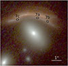 |
Fig. A.1. Silver multiple-image system, showing an arc composed of two blended background sources lensed into multiple images around a cluster member. We identified three multiple-image positions associated with one of the background sources. The system is classified as silver due to its “likely” rather than “secure” spectroscopic redshift and the ambiguous association of the redshift with either of the two blended sources. |
We identified three multiple images of one of the background sources in the silver system, and list their positions and uncertainties in Table A.1.
Observed multiple image positions and positional uncertainties of the silver system.
Appendix B: Overview of mass models
We summarize in Table B.1 the setup of the seven independent modeling approaches, which are described in Sect. 4.
Overview of the lens mass models from the seven independent modeling approaches using the gold image positions as constraints.
Appendix C: Comparison of the models using the gold plus silver samples of lensed images
In addition to the gold samples, both GLAFIC and MrMARTIAN included System 7, classified as a silver sample, in their lens modeling. See Sect. 4.1 and Sect. 4.6 for more details on the lens modeling using the combined gold plus silver samples in GLAFIC and MrMARTIAN, respectively. For both models, the results based on the gold plus silver samples are broadly consistent with those derived from the gold-only samples. In the case of GLAFIC the differences in magnification and time delays between the two models are minimal, typically much smaller than the 1σ statistical uncertainties. While the MrMARTIAN results also remain consistent within the 1σ uncertainties, they exhibit larger differences – on the order of 10–30% – in magnification and time delays. We suspect that, because MrMARTIAN relies solely on the positions of multiple images, the limited constraints near the added analytic halo allow its parameters to vary more significantly within the prior range. We therefore conclude that the inclusion of the silver sample does not significantly affect the time-delay predictions or the estimation of the value of H0 in either modeling approach.
Appendix D: H0 forecast with alternative LENSTOOL I model
As discussed in Section 4.3, the original blinded LENSTOOL I model has very large uncertainties in the model-predicted time delays (in particular, for the pair with the shortest delay, Δt1b, 1a). After the lens model unblinding, these large relative uncertainties were found to be the result of strong degeneracies between time delays and the ellipticity of the mass density profile describing JF-2 – the jellyfish galaxy found to be the most massive in this model – with minimal covariance for other quantities such as the magnifications or image positions. An alternative postblind model (LENSTOOL I-alt) was tested to examine the effect of parameterizing JF-2 as a circular SIS, thereby reducing the relative uncertainty on the model-predicted Δt1b, 1a value (and similarly for Δt2b, 2a). In contrast to the postblind results of MrMARTIAN and WSLAP+ that were due to simple data post-processing issues, the alternate LENSTOOL I model changed its model setup; therefore, it is considered as a new model constructed after unblinding, and is not independent for the comparison with the other models in Sects. 5 and 6. The postblind LENSTOOL I-alt model is shown in Fig. D.1, primarily to demonstrate the consistency between models and rule out errors in processing the LENSTOOL I model results. The alternative model yields only minimal change in the Δt1d, 1a and Δt2d, 2a predictions (not shown); the latter remains an outlier as in Fig. 7 primarily because only a small minority of posterior samples predict an image 2d for both the LENSTOOL I and LENSTOOL I-alt models.
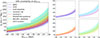 |
Fig. D.1. Same format as Fig. 5, but including the post-blind alternative LENSTOOL I model results, which illustrates improved agreement with the other models. |
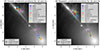 |
Fig. D.2. Predicted positions of SN Encore images 1d and 1e (left panel) and SN Requiem images 2d and 2e (right panel), overlaid on the JWST F200W image. The 1d-1e and 2d-2e pairs of images are merging pairs along the radial arc. The jellyfish galaxies JF-1 and JF-2 (open magenta circles in the left panel) and the BCG alter the positions of the predicted images – even changing image multiplicity, as not all models predict images 1e and 2e (see Tables E.1 and E.2). |
Appendix E: Model predictions of SN Encore and SN Requiem
In Tables E.1 and E.2, we list the model-predicted positions, magnifications and time delays of the multiple images of SN Encore and SN Requiem from the independent lens mass models.
Model-predicted values of position, magnification, and time delay of the multiple images of SN Encore.
Model-predicted values of position, magnification, and time delay of the multiple images of SN Requiem.
Appendix F: Predicted positions of future images of SN Encore and SN Requiem
To understand the origin of the scatter in the predicted positions of images 1d, 1e, 2d and 2e in Figs. 3 and 4, we show in Fig. F.1 the same predicted positions of images 1d and 1e of SN Encore overlaid on the JWST F200W image in the left-hand panel and similarly for images 2d and 2e of SN Requiem in the right-hand panel. The image pair 1d and 1e and the pair 2d and 2e are along the radial arc, where there are nearby foreground cluster galaxies, notably the jellyfish galaxies JF-1 and JF-2. These two jellyfish galaxies and the BCG, depending on their mass distribution, can alter the critical curves and change the predicted image configuration (as noted in Sect. 4.4). Given the limited number of image position constraints (only system 3) near these jellyfish galaxies, the jellyfish galaxies’ mass distributions are currently not well constrained, leading to the different number of image multiplicity and the scatter in the predicted images near the radial arc of SNe Encore and Requiem from the different modeling teams.
All Tables
Observed multiple image positions and positional uncertainties of the silver system.
Overview of the lens mass models from the seven independent modeling approaches using the gold image positions as constraints.
Model-predicted values of position, magnification, and time delay of the multiple images of SN Encore.
Model-predicted values of position, magnification, and time delay of the multiple images of SN Requiem.
All Figures
|
Fig. 1. MACS J0138−2155 as observed through HST and JWST with the following combinations of filters for the color image: F105W+F115W+F125W (blue), F150W+F160W+F200W (green), and F277W+F356W+F444W (red). The positions of the “gold” multiple-image systems are shown with circles. SN Encore is System 1, and SN Requiem is System 2. The foreground (fg) and background (bg) galaxies are marked by cyan diamonds. The dashed squares identify some of the freely optimized cluster members in the lens model, i.e., not constrained by the scaling relations for the cluster members (gray for the ZITRIN-ANALYTIC lens model, maroon for the LENSTOOL I, and that labeled with IDphot = 116 for the GLEE and ZITRIN-ANALYTIC models). The three jellyfish galaxies are labeled with light-green crosses as JF-1, JF-2, and JF-3. |
| In the text | |
|
Fig. 2. Total average surface-mass-density profiles of MACS J0138−2155 as a function of projected distance from the BCG center for the different best-fit strong-lensing models. The vertical lines (at the bottom of the panel) show the observed positions of the 23 multiple images in the gold sample, where the positions of the multiple images of SN Encore and SN Requiem are highlighted in red and blue, respectively. The vertical gray lines (at the top of the panel) mark the positions of the JF-1, JF-2, and bg galaxies, which contribute significantly to the surface mass density at their locations in some models. The inset shows a zoom-in of the region delimited by the dashed rectangle, where the observed multiple images of the two SNe are located. |
| In the text | |
|
Fig. 3. Model predictions for SN Encore’s image positions (left), magnifications (middle), and time delays (right) for a fixed cosmological model (flat ΛCDM with H0 = 70 km s−1 Mpc−1 and Ωm = 0.3 = 1 − ΩΛ). Each row corresponds to one lensed image, as labeled in the top-left corner of each panel in the left column. The coordinate positions are relative to the BCG in arc seconds. The black circle marks the observed image positions of 1a and 1b (left panel in first and second rows, respectively) with the circular radius corresponding to the 1σ positional uncertainty. The insets for the image positions 1a and 1b (left panels) show a zoom-in of the region near the observed image position. The time delays (in days) are relative to image 1a of SN Encore, discovered in November 2023, i.e., Δti, 1a ≡ ti − t1a. |
| In the text | |
|
Fig. 3. continued. |
| In the text | |
|
Fig. 4. Model predictions for SN Requiem’s image positions (left), magnifications (middle), and time delays (right) for a fixed cosmological model (flat ΛCDM with H0 = 70 km s−1 Mpc−1 and Ωm = 0.3 = 1 − ΩΛ), in the same format as Fig. 3. The black circle marks the observed image positions of 2a, 2b, and 2c with the circular radius corresponding to the 1σ positional uncertainty. The time delays (in days) are relative to image 2a of SN Requiem. The measurements of Δt2b, 2a and Δt2c, 2a from Rodney et al. (2021) based on the color curves of the SN Ia template are shown by the vertical line, with the shaded interval marking the 1σ uncertainty. |
| In the text | |
|
Fig. 4. continued. |
| In the text | |
|
Fig. 5. Resulting H0 from different mass models for a range of possible Δt1b, 1a measurements with 10% uncertainty from SN Encore in a flat ΛCDM cosmology with Ωm = 1 − ΩΛ = 0.3. The median values of H0 are shown as solid lines, while the shaded regions indicate the 1σ uncertainty. Left panel: All model predictions overlaid, as indicated in the legend. Right four panels: Subset of the model predictions plotted in the same style as in the left panel, for better visibility. |
| In the text | |
|
Fig. 6. Resulting H0 from different mass models for a range of possible Δt1d, 1a measurements from SN Encore in a flat ΛCDM cosmology with Ωm = 1 − ΩΛ = 0.3. The median values of H0 are shown as solid lines, and the shaded regions indicate the 1σ uncertainty. The assumed 1% uncertainty on Δt1d, 1a is achievable given the long time delay of ∼3000 days. |
| In the text | |
|
Fig. 7. Resulting H0 from different mass models for a range of possible Δt2d, 2a measurements from SN Requiem in a flat ΛCDM cosmology with Ωm = 1 − ΩΛ = 0.3. The median values of H0 are shown as solid lines, and the region delineated by shades indicate the 1σ uncertainty. The relation from the LENSTOOL I model exhibits larger statistical fluctuations since image 2d is predicted in only 16% of the samples for that model (see Table E.2). The assumed 1% uncertainty on Δt2d, 2a is achievable given the long time delay of > 3000 days. |
| In the text | |
|
Fig. 8. H0 inference from SN Encore using the time-delay measurement Δt1b, 1a by Pierel et al. (2026). Top: Inferred H0 distribution from the mass models of the seven modeling teams via blind analysis, where the mass models and the time delay were kept blind to each other throughout and combined after unblinding without modifications. Bottom: H0 from the combined mass model, weighted by each model’s likelihood. The weights were determined before unblinding (see Table 2). Our |
| In the text | |
|
Fig. 9. Comparison of H0 measurements from lensed SNe, local distance ladders, and the CMB (Planck Collaboration VI 2020). The H0 values inferred from the lensed SNe shown in the figure assume a flat ΛCDM cosmological model with Ωm = 0.3 = 1 − ΩΛ, except for the measurement by Grillo et al. (2024) from SN Refsdal, which assumes a more general cosmological model with variable matter density, Ωm, spatial curvature, and dark energy equation of state, w. With the current uncertainties, the H0 from SN Encore is statistically consistent with measurements from SN Refsdal (Kelly et al. 2023; Grillo et al. 2024; Liu & Oguri 2025), SN H0pe (Pascale et al. 2025), and the two distance-ladder approaches of the SH0ES (Riess et al. 2022) and CCHP (Freedman et al. 2025) programs, and the CMB. |
| In the text | |
|
Fig. 10. Forecast of the reappearance dates for SN Encore image 1d (top panel) and SN Requiem image 2d (bottom panel). The prediction from the weighted combination of the seven models is shown in black, with shaded 1σ uncertainties, assuming a 1% time-delay uncertainty. The H0 measurements from Planck Collaboration VI (2020) and SH0ES (Riess et al. 2022) with their 1σ uncertainties are overlaid. Given the long time delays of images 1d and 2d, detecting the reappearance of each SN enables time-delay measurements with ∼1% uncertainty and H0 with 2−3% uncertainty. |
| In the text | |
|
Fig. A.1. Silver multiple-image system, showing an arc composed of two blended background sources lensed into multiple images around a cluster member. We identified three multiple-image positions associated with one of the background sources. The system is classified as silver due to its “likely” rather than “secure” spectroscopic redshift and the ambiguous association of the redshift with either of the two blended sources. |
| In the text | |
|
Fig. D.1. Same format as Fig. 5, but including the post-blind alternative LENSTOOL I model results, which illustrates improved agreement with the other models. |
| In the text | |
|
Fig. D.2. Predicted positions of SN Encore images 1d and 1e (left panel) and SN Requiem images 2d and 2e (right panel), overlaid on the JWST F200W image. The 1d-1e and 2d-2e pairs of images are merging pairs along the radial arc. The jellyfish galaxies JF-1 and JF-2 (open magenta circles in the left panel) and the BCG alter the positions of the predicted images – even changing image multiplicity, as not all models predict images 1e and 2e (see Tables E.1 and E.2). |
| In the text | |
Current usage metrics show cumulative count of Article Views (full-text article views including HTML views, PDF and ePub downloads, according to the available data) and Abstracts Views on Vision4Press platform.
Data correspond to usage on the plateform after 2015. The current usage metrics is available 48-96 hours after online publication and is updated daily on week days.
Initial download of the metrics may take a while.