| Issue |
A&A
Volume 707, March 2026
|
|
|---|---|---|
| Article Number | A132 | |
| Number of page(s) | 8 | |
| Section | Planets, planetary systems, and small bodies | |
| DOI | https://doi.org/10.1051/0004-6361/202556127 | |
| Published online | 16 March 2026 | |
Asteroid characterization using Gaia Data Release 3
II. Taxonomic classification
1
Department of Physics,
PO Box 64,
00014
University of Helsinki,
Finland
2
Astronomical Observatory Institute, Faculty of Physics, A. Mickiewicz University,
Słoneczna 36,
60-286
Poznań,
Poland
3
INAF – Osservatorio Astrofisico di Torino,
10025
Pino Torinese,
Italy
4
Université Côte d’Azur, Observatoire de la Côte d’Azur, CNRS,
Laboratoire Lagrange,
France
5
Yunnan Observatories, Chinese Academy of Sciences,
Kunming,
China
6
Karman+,
11365 Main St,
Broomfield,
CO
80020,
USA
★ Corresponding author: This email address is being protected from spambots. You need JavaScript enabled to view it.
Received:
27
June
2025
Accepted:
27
November
2025
Abstract
Context. We study the taxonomic classification of asteroids observed by Gaia as a continuation of the lightcurve inversion work presented in Paper I.
Aims. We examine the taxonomic classification of asteroids by using both Gaia Data Release 3 (DR3) photometric and spectroscopic data. Particular focus is placed on Ch-class asteroids, as their potentially hydrated nature makes them promising candidates for sample-return missions and the asteroid mining industry.
Methods. We utilized the photometric slopes and geometric albedos (via absolute magnitudes) derived from lightcurve inversion, and the Gaia DR3 spectra (from 418 nm to 770 nm) as classification parameters. We also considered how different parameter sets affect classification accuracies for separate asteroid classes. We classified the asteroids with a combination of linear discriminant analysis and a nearest neighbor classifier.
Results. We achieve a classification accuracy of 92% for known S-class asteroids and an accuracy of 85% for Ch-class asteroids with a known set of 328 asteroids. Given the three classification parameters, tentative class designations for 1668 previously unclassified asteroids are provided in the Mahlke taxonomy. We also show that the photometric slope values vary significantly within asteroid classes, with a standard deviation three to four times the mean slope uncertainties.
Conclusions. We show that the combination of photometry and spectroscopy can be useful in the taxonomic classification of asteroids observed by Gaia. Further studies of the surface roughness at different scales could help clarify the potential of the photometric slope in classification efforts.
Key words: minor planets, asteroids: general
© The Authors 2026
 Open Access article, published by EDP Sciences, under the terms of the Creative Commons Attribution License (https://creativecommons.org/licenses/by/4.0), which permits unrestricted use, distribution, and reproduction in any medium, provided the original work is properly cited.
This article is published in open access under the Subscribe to Open model. This email address is being protected from spambots. You need JavaScript enabled to view it. to support open access publication.
1 Introduction
Photometric and spectroscopic observations of asteroids can reveal information about their surface composition and structure, which in turn can offer insights into the formation of the Solar System (DeMeo & Carry 2014). The taxonomic classification of asteroids has largely relied on the differences in their reflectance spectra, though other parameters have also been explored. The first comprehensive asteroid taxonomy created by Tholen (1984) was based on the geometric albedo and color of asteroids observed in the Eight-Color Asteroid Survey (ECAS). Bus & Binzel (2002) developed a taxonomy using visual spectra from the Small Main-Belt Asteroid Spectroscopic Survey (SMASS) without the geometric albedo, and DeMeo et al. (2009) extended the spectroscopic taxonomy to the near infrared. Mahlke et al. (2022) reintroduced the use of the geometric albedo in combination with spectra to probabilistically assign classes for asteroids.
Asteroid reflectance spectra can be described by their spectral slopes and, oftentimes quite faint, absorption bands. Certain minerals that are known to be abundant in both meteorites and asteroids, such as olivine and orthopyroxene, can have absorption bands that are dominant enough to enable their identification, though different mineral combinations change the position and depth of the bands (Gaffey 1976; Sunshine & Pieters 1998; Reddy et al. 2015). A relatively featureless spectrum throughout the visible and near-infrared wavelengths is characteristic of carbonaceous C-complex asteroids (Bus & Binzel 2002; DeMeo et al. 2009).
Ch asteroids are similar to C asteroids in that they have low geometric albedos and primitive, carbonaceous compositions. However, their spectra differ from the almost featureless C-class spectra as they contain an absorption band at around 700 nm due to oxidized iron (Fe+3) in phyllosilicates, which are minerals formed in the presence of water (Vilas 1994). The potentially hydrated nature of Ch asteroids (Fornasier et al. 2014; Rivkin et al. 2015) makes them a high-value target for asteroid mining and scientific sample return missions.
The albedo- and spectra-based Mahlke taxonomy consists of the S-, M-, and C-complexes, which are comprised of a total of 17 classes. Notably, based on the Tholen classification, many objects that display similar, featureless spectra are subdivided with albedo information into three E, M, and P classes. If an albedo is unavailable, the asteroid is assigned to the X class. We also emphasize that class designation is probabilistic and without constraints on the wavelength range of the spectra. The taxonomic classifications of individual asteroids retrieved from the Solar System Open Database Network, SsODNet (Berthier et al. 2023), contains the most likely class without its probability.
While a spectrum describes how much light is scattered from the surface of an asteroid at a broad wavelength range (and is usually assumed to be independent of time), the lightcurve of an asteroid, i.e., the brightness of the asteroid in a single wavelength band as a function of time, contains information about the shape and spin of the object. The shape and spin characteristics modeled with lightcurve inversion techniques account for the changes in the brightness of the object due to rotational and aspect variations (Muinonen et al. 2020), and therefore constrain the phase function, i.e., the brightness of an asteroid as a function of solar phase angle (the angle between the Sun and the observer seen from the asteroid, α). This in turn enables the determination of its absolute magnitude (Muinonen et al. 2010a). Asteroid phase functions generally exhibit a linear dependence in the magnitude scale at phase angles 10° ≤ α ≤ 50°, which is described by the photometric slope (Muinonen et al. 2022). This photometric slope is mostly inversely correlated with the geometric albedo, but it is also partly influenced by the surface roughness of the asteroid through shadowing effects (Martikainen et al. 2021).
Contrary to the usual ground-based observations of asteroids, which are dense in time, the Gaia Data Release 3 (DR3) contains high-precision sparse-in-time photometric data of more than 150 000 asteroids and low-resolution spectroscopy of more than 60 000 asteroids (Tanga et al. 2023). The wealth of asteroid data allows for the examination of asteroid classification using parameters derived from modeling of asteroid photometry and their respective spectra.
Previous research has demonstrated successful asteroid taxonomic classification with artificial neural networks using simulated Gaia spectra (Penttilä et al. 2021) and Gaia DR3 spectra augmented by the photometric slope derived from the DR3 photometric observations (Uvarova 2024). Uvarova (2024) achieved a mean 80% accuracy in classifying into four asteroid BusDeMeo taxonomic groups (C, S, X, and D). Ge et al. (2024) investigated a larger parameter space for asteroid classification, also utilizing machine learning algorithms. Their best parameter group included Gaia DR3 spectra together with the H, G phase function slope parameter G (Bowell et al. 1989), orbital type, geometric albedo, absolute magnitude, and effective diameter retrieved from the Planetary Data System and the Minor Planet Center, and resulted in a mean accuracy of 92% for six asteroid groups (A, C, D, S, V, and X). Solely including Gaia DR3 spectra, Oszkiewicz et al. (2022) performed binary classification of “V-type” and “other asteroid type” categories by employing machine learning methods, which resulted in a classification accuracy of 92%. Moreover, Cellino et al. (2020) made ground-based spectroscopic observations of a sample of asteroids at similar ranges of wavelength and phase angle as Gaia to support the development of an unsupervised Gaia asteroid taxonomy to be published with the forthcoming Gaia Data Release 4 (DR4).
Drawing on the precise Gaia DR3 photometric data, MacLennan et al. (2025, Paper I) fitted simple triaxial and general convex shapes to the asteroid lightcurves to estimate rotational periods, spin axes, and photometric slopes of the asteroids using the algorithm developed by Muinonen et al. (2020). In this work, we utilized the lightcurve inversion results for the photometric slopes and absolute magnitudes, and combined them with the Gaia DR3 spectra of asteroids for which they are available. We used the absolute magnitudes to calculate geometric albedos by including the effective diameters reported in the SsODNet, and we performed a linear discriminant analysis (LDA) of the combined data. Because we have geometric albedo information computed from the absolute magnitudes determined in the lightcurve inversion, the use of the Mahlke taxonomy (Mahlke et al. 2022) is best suited for the purpose of this research and is used throughout the article. We employed a nearest neighbor classifier optimized for Ch class asteroids to determine how well the parameters classify asteroids in six Mahlke classes (S, Ch, C, P, M, and D). We also provide tentative classifications for asteroids previously unclassified in the Mahlke taxonomy.
The article is structured in the following way. In Sect. 2, we present the Gaia DR3 asteroid data, describe the data selection process, and introduce the methods used in the taxonomic classification. In Sect. 3, we show the results of the combined photometric and spectroscopic analysis and in Sect. 4 we offer insights into potential future developments.
2 Materials and methods
2.1 Gaia DR3
2.1.1 Photometric data
The Gaia DR3 photometry represents brightness in the Gaia G-band filter, which is broader than the commonly used V band. Asteroids were observed down to a magnitude of 21 and mostly in a phase angle range of 10 to 30 degrees. The data processing and selection is explained in full in Paper I, but by selecting asteroids with at least 25 photometric observations (22 815 asteroids) and with quality filtering with a genetic inversion algorithm by Cellino et al. (2024), the number of asteroids with available photometric slopes in the analysis was reduced down to 8659.
2.1.2 Spectroscopic data
We statistically studied the quality and consistency of the Gaia DR3 asteroid spectra against published spectral data in the literature and found that there are a number of difficulties that are due to the way the reflectance spectra of Solar System objects are obtained from Gaia data. First, there are two separate photometers in Gaia: the blue and red photometers (BP and RP) and the joining of the BP and RP observations is not seamless in many cases. Second, there are 16 wavelengths between 374 and 1034 nm given in the spectral data, but the fluxes at both extreme ends of the wavelength range tend to have fairly large uncertainties, depending on the brightness and colors of the objects. The uncertainties remain even after excluding all the spectra with raised quality flags, a fact also confirmed by Gaia Collaboration (2023) and Oszkiewicz et al. (2022).
For the reasons stated above, we decided to use the five wavelengths of 418, 462, 506, 550, and 594 nm in the BP and the four wavelengths of 638, 682, 726, and 770 nm in the RP. Therefore, the wavelength range excludes the diagnostic absorption bands for the minerals orthopyroxene and olivine at around 900 nm and 1000 nm, respectively, but includes the absorption feature wavelength of phyllosilicates at 700 nm that is pertinent to finding Ch asteroids (Fig. 1).
The full DR3 spectroscopic dataset includes 60 518 asteroids. After selecting the asteroids with the highest-quality spectra (with no raised spectral quality flags) and available diameter information from the 8659 asteroids filtered for their photometric data, 1996 objects remain.
 |
Fig. 1 Examples of Gaia asteroid spectra from the most represented classes in our known data set. The spectrum of the example Ch asteroid has a noticeable dip in reflectance around 700 nm corresponding to the absorption feature of phyllosilicates. |
2.2 Photometric slope and absolute magnitude
The process of solving the lightcurve inversion problem is described fully in Paper I, Muinonen et al. (2020), and Muinonen et al. (2022). The main steps to obtaining values for the photometric slope and the absolute magnitude are described in this subsection.
First, triaxial ellipsoids were fitted to the photometric observations and then used as the initial solutions for convex shape fits. In both shape assumptions, a photometric phase function was used that assumes linear dependence on the solar phase angle range 10° ≤ α ≤ 50° in the magnitude scale (Muinonen et al. 2022). The photometric slope β0 quantifies that dependence at α = 20°. The slopes and their uncertainties are computed in Paper I using the MCMC (Markov chain Monte Carlo) method.
We also used the photometric observations to compute the two-parameter H, G12 (Muinonen et al. 2010a) and ![Mathematical equation: $\[H, G_{12}^{*}\]$](/articles/aa/full_html/2026/03/aa56127-25/aa56127-25-eq1.png) (Penttilä et al. 2016) phase functions, which together with the predicted lightcurve maxima from the convex shape solutions are used to derive the absolute magnitudes HGaia for the asteroids (see Paper I). The use of a two-parameter phase function is necessitated by the fact that, due to the properties of the Gaia sky scanning law, Gaia photometric observations of small Solar System bodies are never obtained at very small phase angles. The absolute magnitudes computed from both photometric systems were investigated:
(Penttilä et al. 2016) phase functions, which together with the predicted lightcurve maxima from the convex shape solutions are used to derive the absolute magnitudes HGaia for the asteroids (see Paper I). The use of a two-parameter phase function is necessitated by the fact that, due to the properties of the Gaia sky scanning law, Gaia photometric observations of small Solar System bodies are never obtained at very small phase angles. The absolute magnitudes computed from both photometric systems were investigated: ![Mathematical equation: $\[H, G_{12}^{*}\]$](/articles/aa/full_html/2026/03/aa56127-25/aa56127-25-eq2.png) tends to accommodate the opposition effect of S-class asteroids with shallow phase curves better than H, G12, but possibly overestimates the opposition amplitude for E-class asteroids. Since there are significantly more S-class than E-class objects in the dataset, we decided to use the
tends to accommodate the opposition effect of S-class asteroids with shallow phase curves better than H, G12, but possibly overestimates the opposition amplitude for E-class asteroids. Since there are significantly more S-class than E-class objects in the dataset, we decided to use the ![Mathematical equation: $\[H, G_{12}^{*}\]$](/articles/aa/full_html/2026/03/aa56127-25/aa56127-25-eq3.png) absolute magnitudes in this classification work. We also note that our estimates of the Gaia G-band absolute magnitudes (HGaia) are for a spherical asteroid with a projected area equivalent to the mean projected area of the convex shape.
absolute magnitudes in this classification work. We also note that our estimates of the Gaia G-band absolute magnitudes (HGaia) are for a spherical asteroid with a projected area equivalent to the mean projected area of the convex shape.
2.3 Geometric albedo
We used the absolute magnitudes to calculate geometric albedos, pGaia, for the asteroids with the effective diameters, Deff (the diameter of an equal-volume sphere reported in the SsODNet) and using the relationship (Russell 1916; Pravec & Harris 2007)
![Mathematical equation: $\[p_{\text {Gaia}}=\left(\frac{1246~[\mathrm{km}] ~10^{-0.2 H_{Gaia}}}{D_{\text {eff}}[\mathrm{km}]}\right)^2.\]$](/articles/aa/full_html/2026/03/aa56127-25/aa56127-25-eq4.png) (1)
(1)
The albedo uncertainties were propagated from Eq. (1) using the uncertainties for the absolute magnitudes and diameters.
We note that because the Gaia G-band filter is broader, the scaling factor in the equation is different from the one for the V band (1246 km vs 1329 km). The factor is derived in Appendix A of Paper I.
2.4 Linear discriminant analysis
Linear discriminant analysis is a statistical method used to distinguish between different classes by projecting data onto a lower-dimensional space where the separation between the classes is maximized (Fisher 1936). To achieve this, LDA computes linear combinations of the features, or linear discriminant functions, that best separate the classes. The method is closely related to principal component analysis (PCA), but whereas PCA maximizes variation in the data with the new variables without class information, in LDA the variation between the means of different classes is maximized and the spread within each class is minimized.
First, one needs to compute the covariance matrices within classes c = 1, ..., k:
![Mathematical equation: $\[\boldsymbol{W}=\sum_c\left(n_c-1\right) \boldsymbol{S}_c,\]$](/articles/aa/full_html/2026/03/aa56127-25/aa56127-25-eq5.png) (2)
(2)
where nc is the number of observations in group c and Sc is the covariance matrix of the standardized observations xc for each group. Second, the between-classes covariance matrices are computed:
![Mathematical equation: $\[\boldsymbol{B}=\sum_c n_c(\overline{\boldsymbol{x}_c} \overline{\boldsymbol{x}}_c{}^T),\]$](/articles/aa/full_html/2026/03/aa56127-25/aa56127-25-eq6.png) (3)
(3)
where ![Mathematical equation: $\[\overline{\boldsymbol{x}_{c}}\]$](/articles/aa/full_html/2026/03/aa56127-25/aa56127-25-eq7.png) is the mean vector of xc. Finally, the LDA projection matrix L is given by the eigenvalue decomposition as
is the mean vector of xc. Finally, the LDA projection matrix L is given by the eigenvalue decomposition as
![Mathematical equation: $\[\boldsymbol{L} \boldsymbol{\Lambda} \boldsymbol{L}^{-1}=\boldsymbol{W}^{-1} \boldsymbol{B},\]$](/articles/aa/full_html/2026/03/aa56127-25/aa56127-25-eq8.png) (4)
(4)
where L holds the eigenvectors and the diagonal matrix Λ the eigenvalues of the system. The projection matrix is used to transform the original data into the new variables from which we can choose according to the eigenvalues the most impactful ones to represent the data for classification. In an optimal case, the first few new LDA variables are sufficient to represent the relevant information, thus lowering the dimensionality of the data.
We performed an LDA transform with the scikit-learn Python package for the combination of the photometric slopes, geometric albedos, and eight wavelengths of the Gaia asteroid spectra for all 1996 asteroids. From that set, 328 had a previously identified Mahlke class and were used as the training set in the nearest neighbor classification (see Sects. 2.5 and 3.3). Most of the known asteroids are from the S (n = 116), Ch (54), C (48), P (33), M (23), and D (16) classes, with only a few objects from A (7), L (6), K (5), Z (4), E (3), B (2), and Q (1) classes. There are ten V-class asteroids in this set. Class information for the Mahlke taxonomic classification (Mahlke et al. 2022) was retrieved from the SsODNet with the Python package Rocks.
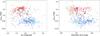 |
Fig. 2 Distribution of the 6205 asteroids for which albedo and slope could be determined. The letter markers represent the corresponding Mahlke class of the asteroid and the gray dots are unclassified asteroids. The number of known asteroids in each class is: S = 135, C = 64, Ch = 61, P = 42, M =30, and D = 23. Most of the unclassifieds are asteroids with diameters less than 10 km. |
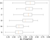 |
Fig. 3 Box plot of photometric slopes for the most represented classes in our dataset. The orange vertical line is the median value in the whole dataset and the box contains the middle half of the data (excluding outliers). |
2.5 Nearest neighbor classification
The k-nearest neighbor (k-NN) classifier inspects the nearest k number of known objects to the object being classified (Cover & Hart 1967). It classifies the object according to the most represented class within its k neighbors. The distance between data points in our approach is the Euclidean distance in the LDA data space. We introduced a k-NN classifier (from the scikit-learn Python package) to our data represented by the three most important LDA variables, and determined how well it classifies the asteroids with a known Mahlke class and with more than ten objects per class. A fifth of the known asteroids were used as the training set and the classification was run 1000 times for k = 3, ..., 10 to examine the accuracy of the classification with different numbers of neighbors and decide on the best value of k for classifying Ch asteroids. The unclassified asteroids with photometric slope, geometric albedo, and Gaia spectral information were classified using the known asteroids as the training set.
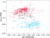 |
Fig. 4 Distribution of the S-, M-, and Ch-class asteroids from Fig. 2 shown with their slope and albedo uncertainties. For the sake of clarity, other classes have been excluded. |
3 Results and discussion
3.1 Geometric albedos and photometric slopes within asteroid classes
The final number of asteroids for which we were able to compute reliable geometric albedos differs from the original 8659 described in Sect. 2.1. The 299 asteroids with convex solutions that were not an improvement on the ellipsoid fit were filtered out (Paper I). Another 2155 asteroids were not considered due to a lack of diameter data in the SsODNet. The geometric albedo results for a final set of 6205 asteroids are shown in Fig. 2, of which 355 have a known Mahlke classification. The S- and M-complex asteroids (including their end members; detailed in Mahlke et al. 2022) have a naturally higher albedo than their carbonaceous counterparts, which is likely due to the higher proportion of multiple scattering from their less-absorbing compositions. For the same reason their photometric slope generally tends to be shallower, resulting in an inverse correlation between the albedo and the slope.
Small-scale surface roughness plays a role at larger phase angles through shadowing by regolith particles (Muinonen et al. 2010b). Consequently, if we assume similar compositions, slopes vary within the same class of asteroids partly due to the surface roughness, and thus slope and albedo alone cannot be used to separate asteroid classes in more detail due to a large overlapping range in slope values. Slope uncertainties do not completely account for the variation as the standard deviation of the values are around three to four times larger than the mean uncertainties. This broad range of slopes in some classes will affect how well the slope can be used in classification. However, most of the S- and M-class asteroids have a slope β0 < 1.9 mag/rad, whereas most of the carbonaceous asteroids have a slope larger than that (Fig. 3).
There is an indication that for the smallest slope values (β0 < 1.5 mag/rad), albedos tend to be lower compared to levels typical for the asteroid class. This is more noticeable in the S-class asteroids, even when taking into account the albedo and slope uncertainties (Fig. 4). For the more primitive asteroid surfaces the albedo is already low and thus the change towards an even lower albedo would not be as steep. The potential trend could be due to large particles creating a smoother surface together with increased packing density, as opposed to a contribution from a regolith consisting of small wavelength-scale particles, resulting in a higher proportion of external reflections and thus a lower albedo. Further research is needed to determine its plausibility. The potential use of the photometric slope as a novel discriminating parameter in the next iteration of a taxonomic classification system is explored in the following sections.
We compared the pGaia values against the values available in the SsODNet for the most represented classes (Fig. 5) and even though the Gaia values are systematically shifted slightly lower due to the wider band filter, the values compare well when accounting for the reported uncertainties. However, there are ten previously classified S-class asteroids with pGaia less than 0.1. Seven of them are low-albedo objects in SsODNet as well. For these asteroids the propagated albedo uncertainties do not explain the low albedos, but erroneous diameters could still account for them. Five of the ten asteroids exhibit S-type spectral behavior (both in the literature and from Gaia), and three resemble P types more. Two outliers are (2918) Salazar and (4036) Whitehouse, which have C-type spectra and high slope values, so they could have been misclassified in SsODNet. We found other low-albedo S candidates with the subsequent k-NN classification, and they are analyzed in more detail in Sect. 3.3.
Additionally, there is one E-class asteroid with an unusually low albedo: (3888) Hoyt. SsODNet gives it an albedo of 0.262, while pGaia = 0.174. The asteroid is thought to be a Phocaea family member, and other previous taxonomic classifications have classified it as S class, so the E-class designation in SsODNet might not be correct. The low albedo results in it mixing with the S-class asteroids in the following LDA (Fig. 6).
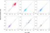 |
Fig. 5 Comparison of Gaia albedos with those reported in the SsODNet (with error bars) for the most represented classes in the known dataset: S, Ch, C, P, M, and D. The dashed line represents equal values. The gray dots are the known asteroids that are not of the class depicted in that particular graph. |
3.2 Linear discriminant analysis
Included in the set of 6205 asteroids with determined photometric slopes and albedos, there were 1996 with Gaia spectra, and from these objects 328 asteroids had an assigned class available in the Mahlke taxonomy. A total of 1668 asteroids did not have class information. The data for the known asteroids plotted in the LDA space of the first three variables is shown in Fig. 6. S-, Ch-, M-, and D-class asteroids group well, which mostly shows in the k-NN classifying results described in the following subsection. L- and K-class asteroids, which are end members of the M-complex (Mahlke et al. 2022), are mixed in with S- and C/Ch-class asteroids, respectively. We find that V-class asteroids, which are part of the Mahlke S-complex, cannot be differentiated from the S-class asteroids. Their geometric albedos are similar to S class and their spectral differences can only be seen outside the wavelength range used in this work. The same occurs for the rare A-class asteroids.
The loadings, i.e., the values of the LDA eigenvectors in the projection matrix L corresponding to the first three variables in LDA space (Fig. 7), show the most emphasis on the albedo and the spectral wavelengths 418 nm, 462 nm, 726 nm, and 770 nm. A modest significance of the photometric slope is present in LDA-1, which also contains its inverse correlation with the albedo. LDA-2 most likely discriminates between the spectral slopes at the end of the wavelength range, whereas LDA-3, to a lesser extent, might act similarly for the shorter wavelengths.
 |
Fig. 6 Asteroids with a previously known Mahlke class (represented by the corresponding letter markers) in the LDA space of the three most significant variables. The LDA shows clear groups of S, M, and C/Ch/P asteroids. D and Ch asteroids are separated with LDA-2, but not LDA-3. While LDA-3 improves the classification success rates (Sect. 3.3), it is not visually noticeable. The number of asteroids in each class is: S = 116, Ch = 54, C = 48, P = 33, M = 23, D = 16, V = 10, A = 7, L = 6, K = 5, Z = 4, E = 3, B = 2, and Q = 1. |
3.3 Nearest neighbor classification
We find that including all three parameters (slope, albedo, spectrum), instead of using other combinations of parameters or only the spectrum, gives the best classification result for S and M classes (by approximately 1–4 and 2–26 percentage points, respectively), whereas the analysis for the Ch class is mostly insensitive to slope and albedo, due to the slope values encompassing a wider range than the values for other classes (Fig. 3) and the albedos overlapping with values within the C, P, and D classes. For D-class asteroids, the benefit is around 8–10 percentage points, but is equaled by the combination of albedo and spectrum. C class is the only one resulting in a better success rate (by 3 percentage points) with only spectra as a classification parameter. Prior artificial neural network classification work by Uvarova (2024) using the combination of Gaia spectra and photometric slope improved the classification of asteroids compared to using only the spectra. We find that the combination of albedo and spectrum always outperforms slope and spectrum (up to 12 percentage points depending on class), but the difference is not discouraging if diameter information is unavailable. We also find that, though visually unconvincing, including LDA-3 in the classification improves the success rates by several percentage points across all the examined classes.
Using the three classification parameters together, the success rates for different values of k in classifying the asteroids with a known class and with group sizes larger than ten are shown in Table 1. The S and Ch classes fare well, but the C-class objects are mixed in with P-class objects in the LDA data and cannot be differentiated. The success rate for M class is surprisingly low given how noticeably it is bordered by S and C classes in the LDA data. At best, the Ch asteroids are classified with an 85% success rate, which is achieved with a k-value of 10. We select this number of nearest neighbors to be used in the algorithm when classifying the asteroids previously without an assigned Mahlke class. We note that while this is an arbitrary number of neighbors, it should not significantly affect the results for our case in which the number of objects in the unclassified dataset is substantially larger than in the known dataset.
After determining the classification accuracies for the previously classified asteroids, we used them as the training set for the classification of the unclassified asteroids. The classification result is shown both in the LDA space and with their photometric slopes and geometric albedos in Fig. 8. The class distributions mostly match the natural albedo cut-off of 0.1 between S-complex and carbonaceous asteroids, thus showing the impact of the geometric albedo in the classification.
There are nine high-albedo (pGaia > 0.4) objects, which we classify as S class. Four of them have S-type Gaia spectra, but the remaining five spectra exhibit flat E-type spectral behavior. All of these five asteroids are in the inner Main Belt, but not in the Hungaria family region.
The classification system assigns an S-class designation for 21 low-albedo (pGaia < 0.1) asteroids. Around half of them have C-type Gaia spectra, so they could be misclassified. The other half have S-type spectra, but due to the uncertainties in their spectra, cannot be confirmed to be low-albedo S-class asteroids.
We examined the situations where asteroids not classified in the Mahlke taxonomy had an assigned class in another taxonomic system (Bus-DeMeo or Tholen). Due to the relatively small number of objects in different Mahlke classes other than S, Ch, C, P, M, and D in our data, the classifier naturally cannot assign a class outside these groups. To roughly assess the plausibility of our classification results, we used the broad distinction of S-, C-, and M-complex asteroids, including their end members. The classification success rates of the previously unclassified asteroids given a class in the Mahlke system with our classifier compared with any previous classification information reported in the SsODNet are 76% (S-complex), 84% (C-complex), and 44% (M-complex). Pure X-class designations are treated by examining the derived Gaia albedos: 0.1 and over are accepted for the M-complex and below 0.1 for the C-complex. The low percentage for the M-complex is due, firstly, to the low classification rate with the LDA data of known M-class asteroids, and secondly, the L and K asteroids being classified as S and C or Ch objects, respectively. Moreover, M-class asteroid compositions may not be as metal-dominated as was previously thought (Rivkin et al. 2000; Masiero et al. 2025).
 |
Fig. 7 Loadings of the LDA transform. The further a value is from zero, the more it contributes to the separation of the classes. The parameters that represent the information used in the analysis are in the following order: photometric slope (β0), geometric albedo (pGaia), and the spectral wavelengths. The spectra were normalized at 550 nm, so the wavelength is excluded. |
 |
Fig. 8 Distribution of asteroids with unknown Mahlke classes classified by the 10-NN classifier with a combination of slope, albedo, and spectrum. The resulting number of asteroids in each class is: S = 747, C = 300, Ch = 201, M = 173, D = 137, P = 108, and V = 2. As there are only two V classifications, they have been given a different symbol to make them more distinguishable in the figure. |
Correct nearest neighbor classification ratios of asteroid classes S, Ch, C, P, M, and D for different k values.
4 Conclusions
We analyzed how well asteroids can be classified with Gaia DR3 spectra, which we restricted to a narrow wavelength range of 418 nm to 770 nm, supplemented by the photometric slope and geometric albedo modeled from the precise Gaia DR3 photometric lightcurve data. The narrow wavelength range of the spectra excludes most absorption bands, which results in an emphasis on the spectral slope. However, the absorption feature of phyllosilicates in the potentially hydrated Ch asteroids is present in the spectral data and assists in their classification.
The LDA of the asteroids with known classes emphasizes the importance of the geometric albedo, which is also demonstrated in the resulting nearest neighbor classification of the asteroids with an unknown classification in the Mahlke taxonomy. The results from including the photometric slope as a classification parameter are more mixed; they are sometimes insignificant but positive in many cases. As the slope is inversely related to the albedo, including it with the albedo and spectrum provides extra emphasis on the albedo but also information on the surface roughness. Further research is needed to work out light-scattering effects on the photometric slope from rough surfaces at different scales.
With more asteroids and, maybe, higher-quality spectra from the forthcoming DR4, further analysis with the photometric slope can be achieved, as well as the detection of more asteroids in the less numerous classes in our current dataset. Nevertheless, reliable taxonomic classification of the objects observed in the Gaia DR4 will be crucial in deriving an accurate Gaia asteroid taxonomy.
In addition to scientific motivations, the detection of Ch-class asteroids in particular is currently of significant interest to the nascent asteroid mining industry. The US, Colorado-based startup Karman+ regards hydrated phyllosilicates as their primary target material to mine for commercial purposes such as satellite refueling and in-space construction (Siltala et al. 2024). Therefore, new methods for detecting asteroids rich in such material are vital to the industry. We note that the current generation of asteroid mining startups has already progressed further than past attempts, with Karman+ preparing to launch a fully privately funded mission, named High Frontier, to a near-Earth asteroid in early 2027 (Velez et al. 2024; Siltala et al. 2024).
Data availability
A table of the results is available at the CDS via https://cdsarc.cds.unistra.fr/viz-bin/cat/J/A+A/707/A132
Acknowledgements
This work has made use of data from the European Space Agency (ESA) mission Gaia (https://www.cosmos.esa.int/gaia), processed by the Gaia Data Processing and Analysis Consortium (DPAC). Funding for the DPAC has been provided by national institutions, in particular the institutions participating in the Gaia Multilateral Agreement. The authors wish to acknowledge the CSC – IT Center for Science Ltd. for computational and data storage resources. The research was supported by the Research Council of Finland grants No. 336546, No. 359893, and No. 347627. AP and KM acknowledge support from Foreign Experts Project (FEP), State Administration of Foreign Experts Affairs of China (SAFEA), with contract No. H20240864. DO acknowledges financial support from grant No. 2022/45/B/ST9/00267 from the National Science Centre, Poland. AC acknowledges support by the Agenzia Spaziale Italiana (ASI) through contracts I/037/08/0, I/058/10/0, 2014-025-R.0, 2014-025-R.1.2015, and 2018-24-HH.0 to the Italian Istituto Nazionale di Astrofisica (INAF), contract 2014-049-R.0/1/2 to INAF for the Space Science Data Centre (SSDC, formerly known as the ASI Science Data Center, ASDC), contracts I/008/10/0, 2013/030/I.0, 2013-030-I.0.1-2015, and 2016-17-I.0 to the Aerospace Logistics Technology Engineering Company (ALTEC S.p.A.), INAF, and the Italian Ministry of Education, University, and Research (Ministero dell’Istruzione, dell’Universita e della Ricerca) through the Premiale project ‘MIning The Cosmos Big Data and Innovative Italian Technology for Frontier Astrophysics and Cosmology’ (MITiC).
References
- Berthier, J., Carry, B., Mahlke, M., & Normand, J. 2023, A&A, 671, A151 [NASA ADS] [CrossRef] [EDP Sciences] [Google Scholar]
- Bowell, E., Hapke, B., Domingue, D., et al. 1989, in Asteroids II, 524 [Google Scholar]
- Bus, S., & Binzel, R. 2002, Icarus, 158, 146 [NASA ADS] [CrossRef] [Google Scholar]
- Cellino, A., Bendjoya, P., Delbò, M., et al. 2020, A&A, 642, A80 [NASA ADS] [CrossRef] [EDP Sciences] [Google Scholar]
- Cellino, A., Tanga, P., Muinonen, K., & Mignard, F. 2024, A&A, 687, A277 [NASA ADS] [CrossRef] [EDP Sciences] [Google Scholar]
- Cover, T., & Hart, P. 1967, IEEE Trans. Inform. Theory, 13, 21 [CrossRef] [Google Scholar]
- DeMeo, F. E., & Carry, B. 2014, Nature, 505, 629 [NASA ADS] [CrossRef] [Google Scholar]
- DeMeo, F., Binzel, R., Slivan, S., & Bus, S. 2009, Icarus, 202, 160 [NASA ADS] [CrossRef] [Google Scholar]
- Fisher, E. 1936, Statist. Discrete Methods Data Sci., 392, 1 [Google Scholar]
- Fornasier, S., Lantz, C., Barucci, M., & Lazzarin, M. 2014, Icarus, 233, 163 [NASA ADS] [CrossRef] [Google Scholar]
- Gaffey, M. J. 1976, J. Geophys. Res., 81, 905 [NASA ADS] [CrossRef] [Google Scholar]
- Gaia Collaboration (Galluccio, L., et al.) 2023, A&A, 674, A35 [NASA ADS] [CrossRef] [EDP Sciences] [Google Scholar]
- Ge, J., Zhang, X., Li, J., et al. 2024, A&A, 692, A100 [NASA ADS] [CrossRef] [EDP Sciences] [Google Scholar]
- MacLennan, E., Pentikäinen, H., Uvarova, E., et al. 2025, A&A, 707, A131 [Google Scholar]
- Mahlke, M., Carry, B., & Mattei, P. A. 2022, A&A, 665, A26 [NASA ADS] [CrossRef] [EDP Sciences] [Google Scholar]
- Martikainen, J., Muinonen, K., Penttilä, A., Cellino, A., & Wang, X. B. 2021, A&A, 649, A98 [NASA ADS] [CrossRef] [EDP Sciences] [Google Scholar]
- Masiero, J. R., Kwon, Y. G., Selmi, E., & Kondapally, M. 2025, Planet. Sci. J., 6, 197 [Google Scholar]
- Muinonen, K., Belskaya, I. N., Cellino, A., et al. 2010a, Icarus, 209, 542 [Google Scholar]
- Muinonen, K., Tyynelä, J., Zubko, E., & Videen, G. 2010b, in Light Scattering Reviews 5: Single Light Scattering and Radiative Transfer (Springer Berlin Heidelberg), 477 [Google Scholar]
- Muinonen, K., Torppa, J., Wang, X. B., Cellino, A., & Penttilä, A. 2020, A&A, 642, A138 [EDP Sciences] [Google Scholar]
- Muinonen, K., Uvarova, E., Martikainen, J., et al. 2022, Front. Astron. Space Sci., 9, 821125 [NASA ADS] [CrossRef] [Google Scholar]
- Oszkiewicz, D., Klimczak, H., Carry, B., et al. 2022, MNRAS, 519, 2917 [Google Scholar]
- Penttilä, A., Shevchenko, V. G., Wilkman, O., & Muinonen, K. 2016, Planet. Space Sci., 123, 117 [Google Scholar]
- Penttilä, A., Hietala, H., & Muinonen, K. 2021, A&A, 649, A46 [NASA ADS] [CrossRef] [EDP Sciences] [Google Scholar]
- Pravec, P., & Harris, A. W. 2007, Icarus, 190, 250 [CrossRef] [Google Scholar]
- Reddy, V., Dunn, T. L., Thomas, C. A., Moskovitz, N. A., & Burbine, T. H. 2015, in Asteroids IV (University of Arizona Press), 43 [Google Scholar]
- Rivkin, A., Howell, E., Lebofsky, L., Clark, B., & Britt, D. 2000, Icarus, 145, 351 [NASA ADS] [CrossRef] [Google Scholar]
- Rivkin, A. S., Thomas, C. A., Howell, E. S., & Emery, J. P. 2015, AJ, 150, 198 [CrossRef] [Google Scholar]
- Russell, H. N. 1916, ApJ, 43, 173 [Google Scholar]
- Siltala, L., Anderson, K., Boyce, F., et al. 2024, in European Planetary Science Congress, EPSC2024-587 [Google Scholar]
- Sunshine, J. M., & Pieters, C. M. 1998, J. Geophys. Res.: Planets, 103, 13675 [Google Scholar]
- Tanga, P., Pauwels, T., Mignard, F., et al. 2023, A&A, 674, A12 [NASA ADS] [CrossRef] [EDP Sciences] [Google Scholar]
- Tholen, D. J. 1984, PhD thesis, University of Arizona, USA [Google Scholar]
- Uvarova, E. 2024, Master’s thesis, University of Helsinki, Finland, available at http://hdl.handle.net/10138/575981 [Google Scholar]
- Velez, D., Anderson, K., Howell, D., et al. 2024, in AAS/AIAA Astrodynamics Specialist Conference, AAS 24-301 [Google Scholar]
- Vilas, F. 1994, Icarus, 111, 456 [NASA ADS] [CrossRef] [Google Scholar]
All Tables
Correct nearest neighbor classification ratios of asteroid classes S, Ch, C, P, M, and D for different k values.
All Figures
|
Fig. 1 Examples of Gaia asteroid spectra from the most represented classes in our known data set. The spectrum of the example Ch asteroid has a noticeable dip in reflectance around 700 nm corresponding to the absorption feature of phyllosilicates. |
| In the text | |
|
Fig. 2 Distribution of the 6205 asteroids for which albedo and slope could be determined. The letter markers represent the corresponding Mahlke class of the asteroid and the gray dots are unclassified asteroids. The number of known asteroids in each class is: S = 135, C = 64, Ch = 61, P = 42, M =30, and D = 23. Most of the unclassifieds are asteroids with diameters less than 10 km. |
| In the text | |
|
Fig. 3 Box plot of photometric slopes for the most represented classes in our dataset. The orange vertical line is the median value in the whole dataset and the box contains the middle half of the data (excluding outliers). |
| In the text | |
|
Fig. 4 Distribution of the S-, M-, and Ch-class asteroids from Fig. 2 shown with their slope and albedo uncertainties. For the sake of clarity, other classes have been excluded. |
| In the text | |
|
Fig. 5 Comparison of Gaia albedos with those reported in the SsODNet (with error bars) for the most represented classes in the known dataset: S, Ch, C, P, M, and D. The dashed line represents equal values. The gray dots are the known asteroids that are not of the class depicted in that particular graph. |
| In the text | |
|
Fig. 6 Asteroids with a previously known Mahlke class (represented by the corresponding letter markers) in the LDA space of the three most significant variables. The LDA shows clear groups of S, M, and C/Ch/P asteroids. D and Ch asteroids are separated with LDA-2, but not LDA-3. While LDA-3 improves the classification success rates (Sect. 3.3), it is not visually noticeable. The number of asteroids in each class is: S = 116, Ch = 54, C = 48, P = 33, M = 23, D = 16, V = 10, A = 7, L = 6, K = 5, Z = 4, E = 3, B = 2, and Q = 1. |
| In the text | |
|
Fig. 7 Loadings of the LDA transform. The further a value is from zero, the more it contributes to the separation of the classes. The parameters that represent the information used in the analysis are in the following order: photometric slope (β0), geometric albedo (pGaia), and the spectral wavelengths. The spectra were normalized at 550 nm, so the wavelength is excluded. |
| In the text | |
|
Fig. 8 Distribution of asteroids with unknown Mahlke classes classified by the 10-NN classifier with a combination of slope, albedo, and spectrum. The resulting number of asteroids in each class is: S = 747, C = 300, Ch = 201, M = 173, D = 137, P = 108, and V = 2. As there are only two V classifications, they have been given a different symbol to make them more distinguishable in the figure. |
| In the text | |
Current usage metrics show cumulative count of Article Views (full-text article views including HTML views, PDF and ePub downloads, according to the available data) and Abstracts Views on Vision4Press platform.
Data correspond to usage on the plateform after 2015. The current usage metrics is available 48-96 hours after online publication and is updated daily on week days.
Initial download of the metrics may take a while.