| Issue |
A&A
Volume 706, February 2026
|
|
|---|---|---|
| Article Number | A58 | |
| Number of page(s) | 13 | |
| Section | Galactic structure, stellar clusters and populations | |
| DOI | https://doi.org/10.1051/0004-6361/202556578 | |
| Published online | 02 February 2026 | |
Substellar initial mass function of Trumpler 14
1
University of Split, Faculty of Science,
Ruđera Boškovića 33,
21000
Split,
Croatia
2
Univ. Grenoble Alpes, CNRS, IPAG,
38000
Grenoble,
France
3
Instituto de Astrofísica e Ciências do Espaço, Faculdade de Ciências, Universidade de Lisboa,
Ed. C8, Campo Grande,
1749-016
Lisbon,
Portugal
4
European Southern Observatory,
Karl-Schwarzschild-Strasse 2,
85748
Garching bei München,
Germany
5
Max-Planck-Institut für Astronomie,
Königstuhl 17,
69117
Heidelberg,
Germany
6
Istituto Nazionale di Astrofisica (INAF) – Osservatorio Astronomico di Palermo,
Piazza del Parlamento 1,
90134
Palermo,
Italy
★ Corresponding author: This email address is being protected from spambots. You need JavaScript enabled to view it.
Received:
24
July
2025
Accepted:
25
November
2025
Abstract
Context. Young, massive stellar clusters offer a prime setting to explore brown dwarf (BD) formation under high densities and intense UV radiation. Trumpler 14 (Tr 14), a ∼1 Myr old cluster located at a distance of 2.4 kpc that is particularly rich in O-type stars, is an ideal target for such a study.
Aims. Our goal is to measure the initial mass function (IMF) in the young massive, high-UV-flux cluster.
Methods. We present the deepest study to date of the IMF in Tr 14, based on Gemini Multi-Conjugate Adaptive Optics System/Gemini-South Adaptive Optics Imager imaging. We constructed the IMF using both the Besançon Galactic model and an observational control field from VISTA for background correction. Completeness was assessed using artificial star tests and applied to the IMF derivation.
Results. We estimated the IMF down to the 20% completeness limit found at ∼0.01 M⊙. Using the control-field-based IMF as our primary result, we find a slope of α = 0.14 ± 0.19 for masses between 0.01 and 0.2 M⊙, and α = 1.72 ± 0.04 for 0.2–4.5 M⊙, where dN/dM ∝ M−α. The low-mass slope is largely influenced by the incompleteness-affected lowest bin; excluding it brings our results into agreement with those for other young clusters. The resulting median for the star-to-BD ratio in the 0.03–1 M⊙ mass range is 4.0, with a 95% confidence interval of 2.8–5.8.
Conclusions. Our analysis reveals that Tr 14 hosts a relatively flat substellar IMF, but this is strongly influenced by the lowest-mass bin, which may be affected by incompleteness. When that bin is excluded, the IMF becomes consistent with those of other regions. The star-to-BD ratio falls within the usually observed ∼3–6 range, indicating that BDs with masses above ∼0.03 M⊙ form with similar efficiencies across environments. However, the relative lack of objects below this threshold suggests that the presence of an environment with both high stellar density and far-UV flux plays a role in shaping the IMF by suppressing the formation of BDs at masses <0.03 M⊙.
Key words: brown dwarfs / stars: formation / stars: low-mass / stars: luminosity function, mass function / open clusters and associations: individual: Trumpler 14
© The Authors 2026
 Open Access article, published by EDP Sciences, under the terms of the Creative Commons Attribution License (https://creativecommons.org/licenses/by/4.0), which permits unrestricted use, distribution, and reproduction in any medium, provided the original work is properly cited.
This article is published in open access under the Subscribe to Open model. This email address is being protected from spambots. You need JavaScript enabled to view it. to support open access publication.
1 Introduction
The study of star formation is of crucial importance in many aspects of astrophysics, for example cosmological evolution at large scales or the formation of planetary systems at smaller scales. The prevailing view is that stars form within star clusters as a result of the gravitational collapse of molecular clouds (Kroupa et al. 2024; Hennebelle & Grudić 2024). Within these clusters, stars and brown dwarfs (BDs) of varying masses emerge, spanning several orders of magnitude, making them an ideal environment for investigating the formation of low-mass stars and BDs.
The initial mass function (IMF) describes the distribution of stellar masses at birth and serves as a fundamental tool for comparing the outcome of star formation in various environments. Above 1 M⊙, the IMF is often considered universal and follows the Salpeter power-law slope (dN/dM ∝ M−α with α = 2.35; Salpeter 1955), although a slightly shallower slope has been observed in some regions (see Bastian et al. 2010 for a comprehensive review). To describe the sub-solar range, Kroupa (2001) proposed a broken power law with α = 0.3 in the 0.01–0.08 M⊙ range and α = 1.3 in the 0.08–0.5 M⊙ range. Additionally, Chabrier (2003, 2005) provides an alternative description, suggesting a log-normal function ( ) with a peak at 0.25 M⊙.
Following the power-law description, observational studies of the low-mass IMF report a range of values for α: α = 0.67 ± 0.23 and α = 0.29 ± 0.22 for Cha-I and Lupus 3, respectively, for the mass ranges 0.02–0.2 M⊙ and 0.04–0.2 M⊙ (Mužić et al. 2025), α = 0.7–1.1 for NGC 2244 for 0.045–0.2 M⊙ or 0.045–0.4 M⊙ (Almendros-Abad et al. 2023), α = 0.51 ± 0.15 for RCW 38 for masses 0.02–0.2 M⊙ (Mužić et al. 2025), α = 0.18 ± 0.19 for masses 0.004–0.19 M⊙ for σ Orionis (Damian et al. 2023), and α = 0.26 ± 0.04 for masses 0.011–0.4 M⊙ for 25 Ori (Suárez et al. 2019). These differences in values could arise from uncertainties affecting the IMF derivation rather than intrinsic variations between clusters. Key factors influencing the determination of the IMF include assumptions about stellar age, cluster distance, theoretical models, membership selection methods, extinction laws, and varying mass ranges for the fits presented here (Scholz et al. 2013).
The low-mass IMF is closely linked to the BD production efficiency. The typical ratio of low-mass stars (0.075–1 M⊙) to BDs (0.03–0.075 M⊙) ranges from 2 to 6 (Mužić et al. 2015, 2017; Andersen et al. 2008; Almendros-Abad et al. 2023). Several mechanisms have been proposed for the formation of BDs, including turbulent fragmentation (Padoan & Nordlund 2002), ejection from multiple systems (Reipurth & Clarke 2001), formation in massive circumstellar discs (Stamatellos & Whitworth 2009), and the photoevaporation of pre-stellar cores by OB-type stars (Whitworth & Zinnecker 2004). However, studies of nearby regions suggest that most massive BDs likely form in a manner similar to stars (see Luhman 2012 for a review), implying the necessity of examining more massive clusters to probe potential environmental variations of the IMF. Several of these theories postulate that the BD formation efficiency depends on environmental factors such as stellar density, gas density, and the presence of massive stars (Luhman 2012). However, this remains an active area of research since it is not yet clear to which extent each of these factors affects the low-mass IMF.
One of the most massive star-forming regions in the Galaxy is the Carina Nebula molecular complex, which contains young massive clusters: Trumpler 14 (Tr 14), Trumpler 15, and Trum-pler 16 (Tapia et al. 2003). Tr 14 contains ∼20 OB-type stars (Shull et al. 2021), which could influence the IMF (Whitworth & Zinnecker 2004). Moreover, we estimate the stellar density of Tr 14 to be ∼103 stars/pc2 (see Sect. 4.4), which is several times denser than the Orion Nebula cluster as found in Almendros-Abad et al. (2023). Estimates of Tr 14’s age vary between <1 Myr and 5 Myr (Tapia et al. 2003; Ascenso et al. 2007; Hur et al. 2012; Itrich et al. 2024), with evidence of two distinct populations: a younger core (<1 Myr) and an older halo (∼5 Myr; Ascenso et al. 2007). The latest spectroscopic analysis, based on MUSE integral field unit observations, places the age of Tr 14 at ∼ 1 Myr (Itrich et al. 2024), which we adopted in our study. The cluster distance was taken as 2.37 ± 0.15 kpc, based on Gaia Early Data Release 3 (Shull et al. 2021), which is in agreement with the results of Göppl & Preibisch (2022), which are based on Gaia Data Release 3 (Gaia Collaboration 2023, Gaia Collaboration 2016). While Ascenso et al. (2007) found a normal extinction law (RV = 3.1) with spatial variations, Hur et al. (2012) suggested an anomalous extinction law towards Carina. The extinction law that we use throughout the paper is from Wang & Chen (2019): RV = 3.1.
Previous studies (Ascenso et al. 2007; Rochau et al. 2011; Hur et al. 2012) of the IMF in Tr 14 have primarily focused on the stellar content, without robust coverage of the low-mass and substellar populations. For example, Ascenso et al. (2007) detect sources down to KS ∼18.5 mag, but they are only 90% complete to KS ∼14.5 mag, corresponding to ∼1–2 M⊙ at 1 Myr depending on extinction and evolutionary models. Hur et al. (2012) report an observational limit of ∼1.6 M⊙. In contrast, Rochau et al. (2011) reach significantly deeper, down to ∼0.25 M⊙. With its rich massive-star population and young age, Tr 14 provides a valuable setting to investigate BD formation and the effect of environmental factors in shaping the low-mass end of the IMF.
In this work we present the most in-depth substellar survey of Tr 14 to date. We used high-resolution near-infrared imaging from the Gemini-South Adaptive Optics Imager. Our analysis focuses on the central ∼1.4′ × 1.4′ region of the cluster, corresponding to ∼0.98 × 0.98 pc2 for a distance of 2.4 kpc. We aimed to characterise the low-mass IMF and evaluate the efficiency of BD formation in a high-radiation environment. We present our observations, the data reduction, and the photometry in Sect. 2. The statistical determination of cluster membership is described in Sect. 3. The derivation of individual object masses and the IMF is presented in Sect. 4. A summary of our results and conclusions are given in Sect. 5.
2 Observations, data reduction, and photometry
2.1 Observations
We observed the Tr 14 cluster in the JHKs filters using the Gemini-South Adaptive Optics Imager (GSAOI; McGregor et al. 2004; Carrasco et al. 2012) assisted by the Gemini Multi-Conjugate Adaptive Optics System (GeMS; Rigaut et al. 2014; Neichel et al. 2014), as a part of programme ID GS-2019A-DD-107 (PI: M. Andersen). Each exposure was 60s, and a total of 25, 15, and 15 exposures were obtained, in J, H, and KS, respectively. Additionally, short exposures of 10s each were taken, with 10 exposures per filter. Three natural guide stars were utilised for the adaptive optics correction; their coordinates are given in Appendix A. All observations were obtained under clear sky conditions. The image quality in the final images for J, H, and KS filters, is 0.14″, 0.13″, and 0.11″, respectively.
2.2 Data processing
The images were processed using standard procedures with the THELI pipeline (Schirmer 2013), and the GSAOI-specific adaptations in Schirmer et al. (2015). Pre-processing included dark subtraction, flat-fielding with domeflats, and the construction of background models using median-stacking of the dithered science images after source masking.
The astrometry and distortion correction were based on the Gaia Early Data Release 3 reference catalogue. The final co-added image was resampled to the nominal GSAOI plate scale of 0.0197″ per pixel. We show the J-band image in Fig. 1.
2.3 PSF fitting photometry
We used SOURCEEXTRACTOR (Bertin & Arnouts 1996) and PSFEx (Bertin 2013) to obtain the point-spread-function (PSF) model and then extracted sources and measured the photometry using PSF-fitting. We tested various parameters to identify the optimal PSF fitting, including BASIS_NUMBER, PSF_SIZE, PSFVAR_KEYS, PSFVAR_GROUPS, PSFVAR_DEGREES, SAMPLE_MINSN. PSFVAR_KEYS and PSFVAR_GROUPS represent the image parameters with which the PSF varies (e.g. X and Y pixel position in the image) and the polynomial group, respectively. PSFVAR_DEGREES stands for the degree of the polynomial of the PSF. We used the same parameters consistently on all the images; the values are given in Table B.1.
Since our field is crowded, for each band, both in long-and short-exposure images, we made two separate extractions, following the concept of ‘hot’ and ‘cold’ detection as outlined in Rix et al. (2004). With just one extraction we were not able to extract both the bright and the faint sources at the same time. Thus, the first extraction (called extraction 1 hereafter) parameters were optimised to gain more sources that are brighter and easier to resolve, and the second extraction (or extraction 2) was done to obtain fainter sources in crowded areas. The most significant parameters for extraction (BACK_SIZE, BACK_FILTERSIZE, DETECT_THRESH, and DEBLEND_MINCONT) affected which sources were detected in the images. The BACK_SIZE parameter defines a cell size in which the local background is estimated using the mode value, while the BACK_FILTERSIZE parameter smooths the background map by applying a median filter. The parameter DETECT_THRESH dictates the threshold above the sky background in units of standard deviation of the background noise. The DEBLEND_MINCONT parameter dictates the contrast for de-blending multiple sources.
The obtained catalogues were cleaned for PSF_MAG=99, FLAGS>=4, and SPREAD_MODEL values deviating by more than 3σ from the mean (see Table B.1 for the exact values). PSF_MAG=99 represents a bad PSF magnitude extraction, for example a saturated source, while SPREAD_MODEL excludes all the deviated and ellipsoidal sources. FLAGS>=4 rejects sources on the edges of the images and with saturation, or corrupted photometric aperture (see SOURCE-EXTRACTOR documentation for more details; Bertin & Arnouts 1996).
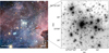 |
Fig. 1 Left panel: image of Tr 14 in the Carina Nebula taken from Preibisch et al. (2011). The black square represents the ∼1.4′ × 1.4′ area studied in this work. Right panel: J-band image of Tr 14 taken with GSAOI. North is up and east to the left. |
2.4 Photometric calibration
Once we obtained the photometry (Sect. 2.3), the extraction 1 and 2 catalogues were combined and then calibrated using the catalogue from Ascenso et al. (2007). The calibration catalogue contains data from two different instruments, with different spatial resolutions. We used only the low-spatial resolution instrument, to avoid possible errors (e.g. matching two stars from our catalogue to one star in the calibration catalogue) in the cross-matching process, and matched it with our catalogue with a tolerance of 0.3″. Moreover, for calibration purposes, we excluded the sources in our catalogue that have another source within 0.5″, to avoid mismatches between the two catalogues. The calibration catalogue from Ascenso et al. (2007) has been calibrated against the Two Micron All Sky Survey (2MASS) photometric system (Skrutskie et al. 2006). We calibrated the photometry using the zero-points (ZPs) only and neglected the colour terms due to them being consistent with zero within the errors. To derive the ZP values for photometric calibration, we took the difference of the instrumental magnitudes from our data and reference magnitudes from the calibrated catalogue, taking measurement errors into account and using 3-sigma clipping. The final ZP was calculated as a weighted average of the surviving data points, with weights determined by the inverse squared errors of both datasets, providing the ZP and its associated uncertainty. As a result, for the long exposure, we get ZPJ = 25.97 ± 0.11 mag, ZPH = 26.18 ± 0.15 mag,  = 25.64 ± 0.16 mag, and for the short exposure ZPJ = 25.99 ± 0.11 mag, ZPH = 26.33 ± 0.11 mag,
  = 25.75 ± 0.10 mag. The photometric uncertainties in individual J, H, and KS catalogues were calculated by combining the uncertainties of the ZPs and the measurement uncertainties supplied by S
ource-Extractor, and are shown in Fig. 2.
The final catalogue for each band was obtained by matching the long and short-exposure catalogues. For the J-band, we used 3-pixel separation, while the rest had 2.5-pixel separation due to the smaller full-width-at-half-maximum of the sources. For the sources that appear in both catalogues, we kept the values with the lower magnitude error. Finally, we cross-matched the catalogues in the three photometric bands using 2.5-pixel separation. We cut 400 pixels off each edge to exclude sources with lower signal-to-noise ratio. The final catalogue contains 1207 sources with photometry in all three photometric bands, 3 additional sources in only J and H bands, 12 sources in only J and KS bands, and 356 sources in only H and KS bands. The first three lines of the catalogue are given in the Table 1 and the full catalogue is provided electronically.
2.5 Completeness
We evaluated the photometric detection completeness through artificial star experiments. Artificial stars were randomly positioned in our images using the source function of Artificial Stellar Populations (A
RTP
OP) Python package (Greco & Danieli 2022). We injected the stars using the PSF model obtained with PSFEx and the parameters listed in Sect. 2.3. We inserted 50 stars at a time and repeated it 10 times, to improve statistics, in steps of 0.2 mag. The extraction used the same parameter values, PSF model, and procedure as in the photometric calibration. Figure 3 shows the fraction of recovered stars in comparison to the inserted artificial ones, as a function of magnitude. The 20% completeness limit is at J = 21.3 mag, H = 20.9 mag and KS = 20.3 mag. This corresponds to the mass of ∼0.01 M⊙, assuming the distance of 2.37 kpc, 1 Myr for the age and combined PARSEC and BT-Settl model (see Sect. 4.1), and with the derived median extinction of the cluster, AV = 2.2 mag (see Sect. 4.1). The 90% completeness limit is at J = 18.4 mag, H = 17.9 mag and KS = 17.7 mag, which corresponds to masses of 0.06–0.08 M⊙. Table 2 summarises our results for the 20%, 50% and 90% limits. The previously deepest data in Tr 14 go down to ∼0.065M⊙ (Itrich et al. 2024) at 30% completeness, not including the core of the cluster.
JHKs catalogue of Tr 14 (extract).
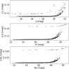 |
Fig. 2 Photometric uncertainties of our catalogue as a function of magnitude. In all bands, two prominent sequences are visible, originating from the long- and short- exposure observations. |
3 Cluster membership
To examine the cluster population, we show two colour-magnitude diagrams (CMDs) of the observations in the first two panels of Fig. 4. The cluster sequence can be fairly well distinguished, with colours J−KS ≈ 1–1.7 mag, but there is a sparsely populated foreground population (to the left of the cluster sequence), and background contamination (to the right) not following the shape of the isochrone and located at the fainter end of the CMD, both of which probably partially overlap with the cluster population. The background population seen in the CMDs in the cluster direction appears to be significantly redder than the cluster sequence. The cluster seems to be located in front of a molecular cloud as seen from the Earth (Ascenso et al. 2007) and it is therefore expected that the background sources suffer larger extinction.
Therefore, in our field of view, we see both the cluster members and field stars contaminating our dataset. We had to be able to differentiate between the two to do a proper analysis of the cluster. Thus, we needed to perform a membership determination. In this section we describe the decontamination of the observations performed using two independent control field (CF) datasets: the Besançon Galaxy model1 and a CF obtained using VIRCAM data from the Visible and Infrared Survey Telescope for Astronomy (VISTA) telescope (Preibisch et al. 2014). The setups for the CFs are explained in Sects. 3.1 and 3.2, respectively, followed by the common decontamination procedure in Sect. 3.3.
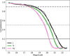 |
Fig. 3 Completeness of the photometry obtained using the artificial star test. The coloured lines represent different photometric bands. The dashed grey line represents the 90% completeness limit, the dotted grey line the 50% completeness limit, and the solid grey line the 20% completeness limit. The thin lines show the completeness curves calculated at the 0.2 mag step, and the thick lines were smoothed using UnvariateSpline of the scipy.interpolate sub-package. |
Magnitudes and masses that correspond to specific completeness limits using the 1 Myr combined PARSEC and BT-Settl (Bressan et al. 2012; Chen et al. 2014; Baraffe et al. 2015) isochrone at 2.37 kpc and AV = 2.2 mag.
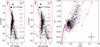 |
Fig. 4 Left and central panels: CMDs. The mean uncertainty is given in the upper-right part of the panels. The solid red line represents the 1 Myr isochrone combined from the PARSEC and BT-Settl models at 1 M⊙ (Bressan et al. 2012; Chen et al. 2014; Baraffe et al. 2015). The reddening vector of Av=3 mag is shown (Wang & Chen 2019). The dashed black line in the first two panels represents the 90% completeness limit, the dotted black line the 50% completeness limit, and the solid black line the 20% completeness limit. Right panel: CCD. The solid red line is the isochrone, as in the CMDs. The dashed red lines are parallel to extinction vectors, while the red crosses represent Av=0, 5, and 10 mag. The dashed-dotted magenta line represents the T Tauri stars’ locus, with the corresponding uncertainties shown as dashed blue lines (Meyer et al. 1997) transformed to 2MASS system using the Carpenter (2001) procedure. The average uncertainty is given in the lower-right corner in the right-most panel; in other panels it is in the top-right. The starting points for the left and middle reddening vector are determined by the masses in the model (<0.5 M⊙ and ≥0.005 M⊙, respectively), while the right reddening vector is from Mužić et al. (2017), adapting the locus of Herbig AeBe stars from Hernández et al. (2005). |
3.1 Decontamination setup with a Galaxy model
To address the contamination with the Besançon Galaxy model presented in Czekaj et al. (2014), as an input we used the central position (l = 287.4107◦, b = −00.5794◦) of our cluster with an area 24.5 times larger than our cluster area on the sky, which was scaled later in the process of decontamination (Sect. 3.3) with the photometric errors given as in Appendix C. We took this size of the area to get a significant number of the expected field stars. The output of the obtained Besançon Galaxy model contains the J-band magnitude, J–H, J–K, and H–K colours, age, mass, coordinates in right ascension and declination, distance and extinction. We transformed the model magnitudes from the Koornneef system to 2MASS using the relations given in Carpenter (2001).
Since the Besançon Galaxy model provides the distances of the simulated stars, we divided the model output into foreground and background populations by comparing those values with the cluster’s location at 2.37 kpc. The foreground population was used for decontamination as is, i.e. without applying any extinction. For the background population, we estimated the values of extinction by reddening the CF photometry until it coincided with the background contaminants seen in the cluster CMD (see Fig. 5). We thus decontaminated the cluster from the background after reddening it with the extinction values of AV = 5, 6, and 7 mag. The decontamination procedure, following the setup described here, is detailed in Sect. 3.3.
3.2 Decontamination setup with VISTA
With the 4-m VISTA of ESO, Preibisch et al. (2014) mapped an area of 6.7 deg2 around the Carina Nebula in the near-infrared J-, H-, and KS -bands, a portion of which we used as a CF. To address the contamination with the CF, we took the shape of a rectangle centred at 10h40m48.00s RA, –59◦31′12.00″ Dec, and 24.5 times bigger than the size of the cluster area. The CF is ∼ 0.4◦ away from our cluster and they have a similar galactic latitude (bCF = −1.118◦, bTr14 = −0.575◦). We took this position and size to get a significant number of field stars. To separate the foreground and background populations of the CF, we used Gaia parallaxes.
We cross-matched our catalogue with Gaia Data Release 3 (Gaia Collaboration 2016, 2023; Babusiaux et al. 2023) to obtain the proper motions and parallaxes, and we performed two cuts. Firstly, we made cuts in proper motion in right ascension and declination, keeping only the most probable members of the cluster, which should behave similarly in the proper motion diagram (PMRA = −6.49±0.60 mas yr−1, PMDec = 2.14±0.58 mas yr−1). We did this by applying sigma clipping using a threshold of 3σ with a maximum of five iterations to iteratively exclude outliers that deviate significantly from the central distribution. This ensures that the derived statistical parameters reflect the intrinsic kinematic properties of the population, minimising the impact of contaminants or measurement errors. Secondly, we applied an additional brightness cut on the subset obtained from the first selection, keeping only the brightest (<16 mag) objects to calculate the weighted mean parallax and parallax error. This value was then used to identify and reject foreground objects in the Tr 14 catalogue based on a parallax zeta score >2. We calculated the zeta score with the expression  , where ω and σω are the parallax and the uncertainty for each star, while the
  and σ are the weighted mean and uncertainty of the whole sample. We were left with a dataset of our cluster that contains probable cluster members as well as the background contaminants.
We then made the same cut based on the parallax zeta score in the VISTA CF catalogue, which we previously cross-matched with Gaia Data Release 3, to keep only the subset that corresponds to a probable background. We show the results of these cuts in Fig. 6. To this VISTA CF catalogue with removed foreground objects, we applied different amounts of extinction (AV = 6.5, 7, and 7.5 mag; see Fig. 5), which we then used in the procedure explained in Sect. 3.3.
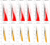 |
Fig. 5 CMDs for the Besançon model (upper panels) and the VISTA CF (lower panels). The black dots show all the objects in the line of sight of Tr 14. The grey dots are the model foreground, while the red ones are the reddened model background. The orange dots represent the reddened CF. The amount of reddening is given above each panel. Each extinction is chosen to decontaminate the most amount of background sources. |
3.3 Statistical determination of membership
To statistically determine the cluster membership, after the independent setups for the CFs in Sects. 3.1 and 3.2, we applied the procedure from Mužić et al. (2019), which is summarised as follows:
The CMD containing the cluster and the CF, as in Fig. 5 (upper panels if we use the Besançon model as the CF and lower panels if we use VISTA as the CF), is divided in a grid with cell sizes ∆colour and ∆magnitude.
For each cell, the expected number densities of stars in the cluster field of view and in the CF (either from the Besançon model or from VISTA) are calculated. The densities are then scaled for different on-sky areas of the cluster and the CF.
he expected number of field objects in each cell is then randomly removed from the cluster population.
Each object in the CMD is represented with a Gaussian probability distribution in the space of colour and magnitude, with the width being determined by the photometric uncertainties. The part of the Gaussian that lies within the cell is then integrated and summed to get the expected number of objects for each cell. Cell sizes are determined in a way to have good statistics of cluster members and CF objects in each cell. We then removed from the cluster field as many sources as computed in the CF in each cell. The specific objects to be removed are chosen randomly. We used different cell sizes with ∆magnitude = (0.4, 0.5, 0.6) mag, which results in Nmag = 3 different magnitude bin sizes and ∆colour = (0.3, 0.4) mag, yielding Ncol = 2 colour bin sizes. Additionally, to improve accuracy for the objects laying at the edges of our cells, for each magnitude-colour combination, we shifted the cell centre for 0.0, 1/3, and –1/3 of the cell size in each dimension. This created Ns = 3 · 3 = 9 cell centre configurations. We repeated the decontamination procedure for each combination of various parameters, namely cell sizes and cell centres, as well as the applied reddening. We looked at Ncmd = 2 CMD types (J, J–K,J−H) for  = 3 extinction values as shown in Fig. 5. This results in Nmag · Ncol · Ns · Ncmd ·
  = NL = 324 lists of potential cluster members, which contain IDs of catalogue sources that we later employed in the procedure for the IMF determination of the cluster. We calculated the probability of each star in the catalogue being a cluster member by counting the number of times it appears in all lists and then dividing by the total number of lists. This methodology follows the similar approach previously applied in other young clusters such as NGC 2244 (e.g. Mužić et al. 2019), and has been validated through spectroscopic analysis by Almendros-Abad et al. (2023), demonstrating its robustness in separating cluster and field populations. The resulting probabilities are shown in Fig. 7, where we use the VISTA (bottom panel) and the Besançon model (upper panel) as CFs in the decontamination method. In the bottom panel, the foreground population appears as high-probability members since for the decontamination with VISTA we cross-matched our catalogue with Gaia, which is much shallower than our photometry, and thus the sample is limited. We then removed the foreground objects, which are known to contribute to contamination based on their Gaia parallaxes, as explained in Sect. 3.2.
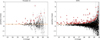 |
Fig. 6 Parallax versus the G magnitude band of Tr 14 (left panel) and the VISTA CF (right panel). Red crosses represent the objects that are ruled out from being part of the foreground of Tr 14 (left panel) and CF (right panel). Black dots represent the objects of the cluster (in the left panel) and CF (in the right panel), while the grey error bars are parallax errors. To remove the foreground, we set the zeta score for the parallax to >2. The dashed orange line represents the mean cluster parallax, and the orange rectangle is ±σ of the mean cluster parallax. |
4 Results and discussion
4.1 Extinction and masses
To derive the IMF of our cluster, we had to estimate the masses of the cluster members. We used evolutionary models to get these values. To obtain extinction and masses, we de-reddened our sources to the J, J–H isochrone in the CMD, as in Mužić et al. (2017). The full CMD and colour-colour diagram (CCD) are shown in Fig. 4. We combined the PARSEC and BT-Settl models at 1 M⊙ to a 1 Myr isochrone (Bressan et al. 2012; Chen et al. 2014; Baraffe et al. 2015) as in Mužić et al. (2019).
First, we generated 1000 magnitude values for each source assuming a normal distribution, where the standard deviation is the photometric uncertainty. We checked whether the source with the uncertainties was inside or crossing the model limits (solid red and dotted red lines in Fig. 4 in the CCD); otherwise, the mass was not derived. The extinction was then derived by de-reddening in the CMD to the 1 Myr isochrone in these 1000 runs. The mass was obtained by interpolating the mass-magnitude relation corresponding to the model isochrone.
An example of the mass and extinction derivation procedure of one of the sources is shown in Fig. 8. The right extinction line delimits we would expect to see T Tauri (Meyer et al. 1997) and Herbig AeBe (Hernández et al. 2005) stars (we would expect to see them to the left of this line). However, as argued in Mužić et al. (2019), the excess coming from the circumstellar disc of the classical T Tauri or Herbig AeBe stars appears to have a negligible impact on the IMF; thus, we did not attempt to correct for it. Additionally, mass and extinction histograms are plotted. In these runs, it is possible to obtain negative AV; however, this is not physical. To correct for it, without skewing the distributions, only data points with AV >= 0 are used to estimate the IMF.
As a result of this procedure, we get the mass distributions, median mass, median and mean extinction with its standard deviation for each source in the catalogue. The mass distributions are later used to obtain the IMF.
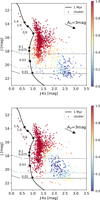 |
Fig. 7 Cluster membership probability determined using the model (upper panel) and the VISTA CF (lower panel) as a CF in the process of decontamination. The solid black line represents the 1 Myr isochrone combined from the PARSEC and BT-Settl models at 1 M⊙ (Bressan et al. 2012; Chen et al. 2014; Baraffe et al. 2015). The reddening vector of AV=3 mag is shown. The dashed grey line represents the 90% completeness limit, the dotted grey line the 50% completeness limit, and the solid grey line the 20% completeness limit. |
4.2 Initial mass function
We aimed to derive the IMF from a set of mass distributions, obtained as described in Sect. 4.1, using the lists containing IDs of catalogue sources that remain after the decontamination procedure described in Sect. 3.
Each star’s mass is represented by a mass distribution that is smoothed using a Gaussian kernel density estimation. From the mass distribution of each star, we drew a sample of N1 = 100 values per object; this resulted in 100 different mass distributions for the entire sample. Next, for each of the N1 resampled sets, bootstrap (random samplings with replacement) is performed N2 = 100 times to account for statistical fluctuations. This results in N1 · N2 individual mass distributions. During each iteration, we evaluated the IMF as a histogram with variable bin sizes, chosen to contain roughly the same number of objects and save it. The same bins were used in each iteration. We corrected this mass function for completeness by dividing each star in the bin individually with its corresponding completeness value. We excluded all the sources with completeness <= 20% from the calculation of the IMFs because we did not want to be biased by the faint objects that have low completeness. To ensure the robustness of the derived IMF, we then averaged the N1 · N2 · NL IMFs obtained and calculated the standard deviation to estimate the uncertainty of each bin.
The results for the IMFs are shown in Fig. 9 and summarised in Table 3. The obtained slope α (dN/dM ∝ M−α) when fitting between 0.01 and 0.2 M⊙ differs depending on whether we do the decontamination with the Besançon model or the VISTA CF: using the Besançon model, we get α = 0.03 ± 0.24, whereas using the VISTA CF, we obtain α = 0.14 ± 0.19. When fitting the IMF between 0.2 and 4.5 M⊙, we find α = 1.72 ± 0.04 for both decontamination methods.
We note that the decontamination primarily affects the lowest-mass bin, whereas above this limit the results remain very similar. On the low-mass part of the IMF, the Besançon model may be overestimating the number of contaminants. This could originate from Tr 14 being a cluster located in a young star-forming region, implicating the presence of nebulosity and extinction. The approach using VISTA as the CF is more realistic because it directly samples the actual background and environmental conditions, whereas the Besançon model relies on assumptions that may not fully take into account local conditions. In particular, the model does not include explicit spiral-arm overdensities along this line of sight, such as the Carina arm, which could also cause it to underestimate the number of field stars near the cluster distance. However, even if such an over-density were included, it would likely be uniformly distributed across the CMD and thus would not affect our decontamination result, especially in the lowest-mass bin where the largest difference relative to the VISTA CF is observed. Meingast et al. (2016) find that the Besançon model overestimates number of faint (KS > 19 mag) and bright (KS < 10 mag) objects, which could explain the results that we find. However, our approach with the VISTA CF could, due to its position, sample different parts of the Milky Way and thus potentially not see general Carina contamination, in addition to underestimating the foreground contamination, since Gaia does not have any parallax measurement for faint objects as explained in Sect. 3.2. Overall, the true number of contaminants, and consequently the resulting IMF slope, likely lies between the values inferred from the VISTA and Besançon model decontamination approaches, with the two CFs yielding consistent results when the lowest-mass bin is excluded.
In the dN/dlogM representation of the IMF (Chabrier 2003), as shown in Fig. 10, we fitted a log-normal function. We derived a characteristic mass mc = (0.20 ± 0.02) M⊙ and σ = 0.45 ± 0.03 with the decontamination approach using the Besançon model, while for VISTA we get mc = (0.20 ± 0.02) M⊙ and σ = 0.50 ± 0.03. Rochau et al. (2011) studied the central ∼1 × 1 arcmin2 of Tr 14. They report a higher characteristic mass of ∼0.52 M⊙. For the dN/dM power law, they find α = 0.37±0.32 for masses 0.25–0.5 M⊙ and α = 1.52 ± 0.3 for masses 0.5–3.2 M⊙. In contrast to Rochau et al. (2011), we do not find statistically significant evidence of a break in the IMF slope around 0.5 M⊙. This may be due to our extended mass coverage and improved completeness, especially below 0.5 M⊙. Compared to Damian et al. (2021), who find mc = (0.32 ± 0.02) M⊙ and σ = 0.47 ± 0.02 from a sample of nine clusters, our characteristic mass is lower, while the width of the distribution (σ) is similar or slightly broader. This shift towards lower mc may reflect differences in environmental conditions specific to Tr 14, or it may result from our deeper completeness and sensitivity to lower masses, particularly in the BD regime.
The results we obtain for the high mass part are similar to other studies in this mass range: for RCW 38, α = 1.48 ± 0.08 for masses 0.2–20 M⊙ (Mužić et al. 2017); for σ Ori, α = 1.73±0.16 for masses 0.35–19 M⊙ (Peña Ramírez et al. 2012); but shallower than: 25 Ori where α = 2.50 ± 0.11 for masses 0.4–13.1 M⊙ (Suárez et al. 2019), NGC 2244 where α = 2.3 ± 0.3 for masses 1.5–20 M⊙ (Mužić et al. 2022) and for the standard Salpeter slope (α = 2.35). Our derived substellar IMF slope is significantly shallower than the typical values reported in the literature. For example, α = 0.67 ± 0.23 in Cha-I for masses 0.02–0.2 M⊙ and α = 0.51 ± 0.15 in RCW 38 for masses 0.02–0.2 M⊙ (Mužić et al. 2025); α = 0.7 ± 0.12 for masses 0.045–0.2 M⊙ in NGC 2244 (Almendros-Abad et al. 2023). Compared to these regions, our results suggest a flatter distribution of substellar objects, implying a lower relative BDs with respect to stars. However, we find α = 0.33 ± 0.22 and α = 0.26 ± 0.16 for the VISTA and Besançon model CF in the 0.03–0.2 M⊙ mass range, similar to α = 0.29 ± 0.22 in Lupus 3 for masses 0.04–0.2 M⊙ (Mužić et al. 2025), α = 0.26 ± 0.04 for masses 0.011–0.4 M⊙ in 25 Ori (Suárez et al. 2019) and α = 0.18±0.19 for masses 0.004–0.19 M⊙ in σ Ori (Damian et al. 2023). While our lowest-mass range 0.01–0.2 M⊙ yields particularly shallow slopes, this result is based on the least massive point, where the incompleteness is highest and uncertainties are largest. If this point is excluded, the remaining slope values are consistent with those reported for other young clusters. The results are illustrated in Fig. 11 (see e.g. Hennebelle & Grudić 2024 for a more comprehensive summary).
 |
Fig. 8 Example of mass derivation for one of the sources. Left panels: 1 Myr isochrone (solid red line) combined from the PARSEC and BT-Settl models at 1 M⊙ mass (Bressan et al. 2012; Chen et al. 2014; Baraffe et al. 2015) and the source with its error bars (solid orange cross). The grey dots represent the generated magnitude points from 1000 runs. In the first panel, a line parallel to the extinction vector would show where the mass lies on the model. In the second panel, the dotted red lines are parallel to the reddening vectors. Red crosses mark the extinction in 5 mag steps from 0 to 15 mag. Right panels: mass and extinction distribution, respectively, obtained from 1000 runs. |
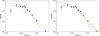 |
Fig. 9 dN/dM representation of the IMF of Tr 14 after decontaminating with the Besançon model CF (left panel) and the VISTA CF (right panel). Black dots with corresponding uncertainties are after correcting for completeness, while grey circles are the bins before the correction. The dotted black line represents the standard mass function from Kroupa (2001). The power-law break is at ∼0.2 M⊙. For the solid blue line fit in the left panel, we get the slope of α = 0.03 ± 0.24, and for the solid orange line α = 1.72 ± 0.04. For the solid blue line fit in the right panel we get a slope of α = 0.14 ± 0.19 and for the solid orange line α = 1.72 ± 0.04. |
IMF slopes (where dN/dM ∝ M−α) derived for the combined BT-Settl and PARSEC evolutionary model, and different mass ranges, and for the two decontamination strategies.
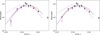 |
Fig. 10 dN/d(logM) representation of the IMF of Tr 14 after decontaminating with the Besançon model CF (left panel) and the VISTA CF (right panel). Black dots with corresponding Poisson uncertainties are the result after correcting for completeness, while grey circles represent the IMF before the correction. The dotted black line represents the standard mass function from Kroupa (2001), the dashed black line the mass function from Chabrier (2005), and the solid magenta line our log-normal fit of the IMF. |
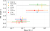 |
Fig. 11 Alpha plot for the studies we compare our results to in the discussion. Each region is marked in different colours and symbols, as given in the legend, with its corresponding error bars for the α. Tr 14 values are from this study. The two Tr 14 points at low masses correspond to the two different mass ranges used to compute the IMF slope. Horizontal bars represent the mass ranges over which the corresponding α values were derived and do not indicate uncertainties. |
4.3 Testing IMF assumptions
4.3.1 Dynamical evolution
To interpret the observed mass function in our field of view as IMF, it is necessary to assume that no significant fraction of cluster members resides outside our observed region, and that dynamical evolution has not substantially altered the mass distribution since formation. While such assumptions are generally justified for very young clusters, Tr 14 is both massive and compact, with a half-mass radius of 1.5–1.8 pc and a total stellar mass of several thousand solar masses (Shull et al. 2021). Its crossing time is estimated at ∼0.7–0.8 Myr, and its two-body relaxation time ranges from 40 to 80 Myr (Shull et al. 2021). Given the cluster’s age of ∼1 Myr, this places it just beyond one crossing time but still far from being dynamically relaxed. This suggests that dynamical effects such as the ejection of members or significant radial redistribution (especially for low-mass objects) are unlikely to have strongly influenced our sample. While Sana et al. (2010) report signs of mass segregation, most likely due to dynamical friction, among stars more massive than ∼10 M⊙, Shull et al. (2021) argue that even the most massive stars (30–80 M⊙) are unlikely to have undergone significant segregation within the cluster’s 1–3 Myr lifetime. While this supports the idea that our sample, limited to lower-mass stars and BDs in the central region, is likely to still reflect the IMF, some degree of primordial mass segregation cannot be ruled out. A wider field study would be needed to verify whether spatially dependent effects like mass segregation influence the mass function at larger radii.
4.3.2 Crowding
To assess the potential influence of crowding and the halos of bright stars on the derived IMF, we compared the IMFs extracted from two distinct regions within our field of view. We defined the most crowded region by drawing a rectangle over the central area of the image, while the rest of the field encompassing less crowded surroundings was treated as a separate region for comparison. We computed the photometric completeness separately for each region and subsequently derived their respective IMFs. We found only small differences between the two IMFs. For the mass range 0.01–0.2 M⊙, we measured slopes of αVISTA,inside = 0.07 ± 0.18 and similarly αVISTA,outside = 0.16 ± 0.22, while for the Besançon model CF αmodel,inside = −0.07 ± 0.22 and αmodel,outside = 0.05 ± 0.26. In the mass range 0.2–4.5 M⊙, we find αVISTA,inside = 1.68 ± 0.06 and αVISTA,outside = 1.76 ± 0.04, while for the Besançon model CF αmodel,inside = 1.65 ± 0.05 and αmodel,outside = 1.77 ± 0.05. These results indicate that crowding and the presence of bright stellar halos do not significantly bias our IMF determination.
4.3.3 Evolutionary models
To be able to cover the full range from the substellar to high stellar masses, in our analysis we used a BT-Settl and PARSEC isochrones combined into a single isochrone at 1 M⊙. To estimate the impact of this combination, we evaluated the IMF with the two isochrones separately, within the common mass range. The results are given in Table 4. We see that with the PARSEC (Bressan et al. 2012) evolutionary model we have an overabundance of low-mass sources in comparison to the results obtained using BT-Settl evolutionary models (Baraffe et al. 2015). Using the PARSEC isochrone, in the process of deriving masses, a large portion of objects will be crossing the lowest point on the isochrone, creating the artificial abundance of low-mass objects. We thus conclude that using a combined isochrone does not produce any anomalous effects at the intersection of the isochrones, and that the IMF is consistent with both models.
IMF slopes (where dN/dM ∝ M−α) derived for different evolutionary model combinations in the 0.2–1.2 M⊙ mass range.
4.4 Star-to-BD ratio
To calculate the star-to-BD ratio, we used the same method as in the IMF derivation, up to the point where we binned the data. At this point, we instead counted the number of sources in the mass ranges 0.03–0.075 M⊙ for the BDs and 0.075–1 M⊙ for the stars and correct for completeness, restricting only to sources with completeness ≥20%. The median star-to-BD that we obtain using the VISTA CF is 4.0, with a 95% confidence interval of 2.8–5.8, while for the Besançon model it is 4.3 with the 95% confidence interval of 3.1–6.0. As stated previously, we consider the result with the VISTA CF to be more realistic. This result is in agreement with the star-to-BD ratios in RCW 38 (2.0±0.6), Cha-I (3.2–4.8), and Lupus 3 (2.1–4.5) from Mužić et al. (2025). Our result is in agreement with Andersen et al. (2008), who report star-to-BD ratios in different regions in the range 3.3–8.5.
To place Tr 14 in context of different environments, we estimated its surface density and far-UV (FUV) flux from massive stars. We calculated a mean surface density of ∼1000 stars/pc2 by dividing the number of sources in our field of view by the area. To estimate the FUV radiation, we followed the process outlined in Mužić et al. (2025). We derive a flux of approximately 105.54 G0.
The Fig. 11 in Almendros-Abad et al. (2023) shows that the star-to-BD ratio does not significantly vary with stellar surface density, nor with the presence of OB stars. Their analysis includes clusters with surface densities in ∼10–1000 stars pc−2 range, including the Orion Nebula cluster, RCW 38, NGC 2244, Lupus 3, Cha-I, NGC 1333 and IC 348. Tr 14 is on the high end of this range, placing it among the densest clusters examined and only surpassed by RCW 38.
In terms of FUV radiation, Fig. 8 of Mužić et al. (2025) presents the median FUV flux for Lupus 3, Cha-I, NGC 2244, CrA, NGC 1333, and RCW 38. Tr 14, with its estimated flux of 105.54 G0, exceeds all the clusters in their sample, including RCW 38 (∼105.3 G0).
Despite this extreme environment, high density and high FUV flux, our measured star-to-BD ratio evaluated for the mass range 0.03–0.075 M⊙, lies between ∼3 and 6. This range is comparable to those observed in both low- and high-density environments in Almendros-Abad et al. (2023) and Mužić et al. (2025), suggesting that the star-to-BD ratio in Tr 14 does not significantly differ from other regions in this mass range. However, we note that the IMF we derived is significantly flatter than those in the comparison regions. This apparent contradiction can be explained when considering the slope uncertainties and excluding the lowest-mass bin, which drives much of the flattening; with that bin removed, the slope becomes more consistent with other clusters. However, if we were to include lower-mass BDs (<0.03 M⊙), where our IMF shows a clear deficit, we would likely start to see deviations from the trend, indicating a possible environmental influence on the formation efficiency of the lowest-mass substellar objects. Interestingly, while Almendros-Abad et al. (2023) propose that OB stars may enhance BD formation in NGC 2244, our results from the denser and more UV-intense environment of Tr 14 do not support this scenario, pointing instead to a potential suppression. It may be that a combination of high density and intense radiation fields inhibits the fragmentation processes needed for efficient formation of very low-mass objects.
5 Summary and conclusions
Using GSAOI/GeMS observations, we have presented the most complete mass function in Tr 14 to date, covering objects from the substellar regime up to 4.5 M⊙. Our final catalogue contains 1207 sources in the J, H, and KS bands. The data are 50% complete down to 0.02 M⊙ and 20% complete down to 0.01 M⊙. Because there are both field stars and cluster members in our dataset, we statistically decontaminated the catalogue using either the Besançon model or observational data from the VISTA telescope as a CF. Masses and extinctions were obtained from comparisons to the evolutionary models from Bressan et al. (2012), Chen et al. (2014), and Baraffe et al. (2015). The resulting IMF below 0.2 M⊙ differs depending on whether we use the Besançon model or VISTA for the decontamination process. We believe that the Besançon model overestimates the contamination and therefore prefer the results obtained using the observational CF.
Using the VISTA CF, we find the slope of the high-mass part of the IMF (∼0.2–4.5 M⊙) to be α = 1.72 ± 0.04, which is similar to other young star-forming regions but shallower than the standard Salpeter slope. For the low-mass end of the IMF (∼0.01–0.2 M⊙), we find a relatively shallow slope of α = 0.14 ± 0.19. While this appears significantly flatter than values reported for other regions, the comparison should be treated with caution: not only do we probe a slightly different mass range than most studies, but the lowest-mass bin in this mass range is also the most affected by incompleteness, leading to larger uncertainties. If the least massive point is excluded, the remaining slope values are consistent with those reported for other young clusters.
Nonetheless, the observed flattening could suggest that the number of BDs declines steeply with decreasing mass, especially below 0.03 M⊙, in turn suggesting a lower formation efficiency for substellar objects in this environment. The cause of this suppression is unclear but may relate to the specific environmental conditions of Tr 14. Its mean surface density of ∼1000 stars/pc−2 lies between that of NGC 2244 (lower) and RCW 38 (higher), yet the substellar IMF we find is much flatter than in either of those regions. In terms of FUV flux, Tr 14 is exposed to stronger radiation fields than both NGC 2244 and RCW 38, and this may inhibit the formation or survival of its lowest-mass BDs. Though we cannot yet conclude this definitively, our findings highlight the importance of considering both stellar density and radiative feedback in shaping the low-mass end of the IMF.
Finally, we find that the star-to-BD ratio is 4.0 (with a 95% confidence interval of 2.8–5.8) in the mass range 0.03–1 M⊙, which is within the expected range of ∼3–6 found in the literature. This places Tr 14 near the middle of the observed distribution of star-to-BD ratios, suggesting that in this specific mass range, BDs form at least as efficiently as low-mass stars, consistent with other environments. However, our IMF shows a significantly flatter slope and a deficit of objects at even lower masses (below 0.03 M⊙), which are not included in this ratio. This may indicate that environmental effects primarily influence the formation efficiency of the lowest-mass BDs.
Data availability
Table 1 is available at the CDS via https://cdsarc.cds.unistra.fr/viz-bin/cat/J/A+A/706/A58.
Acknowledgements
This work was supported by/supported in part by the Croat-ian Science Foundation under the project number HRZZ-MOBDOK-2023-9579. K.M. acknowledges support from the Fundação para a Ciência e a Tecnologia (FCT) through the CEEC-individual contract 2022.03809.CEECIND, and the Scientific Visitor Programme of the European Southern Observatory (ESO) in Chile. V.A.-A. acknowledges support from the INAF grant 1.05.12.05.03. Based on observations (programme ID GS-2019A-DD-107, PI: M. Andersen) obtained at the international Gemini Observatory, a programme of NSF NOIR-Lab, which is managed by the Association of Universities for Research in Astronomy (AURA) under a cooperative agreement with the U.S. National Science Foundation on behalf of the Gemini Observatory partnership: the U.S. National Science Foundation (United States), National Research Council (Canada), Agencia Nacional de Investigación y Desarrollo (Chile), Ministe-rio de Ciencia, Tecnología e Innovación (Argentina), Ministério da Ciência, Tecnologia, Inovações e Comunicações (Brazil), and Korea Astronomy and Space Science Institute (Republic of Korea). This work has made use of data from the European Space Agency (ESA) mission Gaia (https://www.cosmos.esa.int/gaia), processed by the Gaia Data Processing and Analysis Consortium (DPAC, https://www.cosmos.esa.int/web/gaia/dpac/consortium). Funding for the DPAC has been provided by national institutions, in particular the institutions participating in the Gaia Multilateral Agreement.
References
- Almendros-Abad, V., Mužić, K., Bouy, H., et al. 2023, A&A, 677, A26 [NASA ADS] [CrossRef] [EDP Sciences] [Google Scholar]
- Andersen, M., Meyer, M. R., Greissl, J., & Aversa, A. 2008, ApJ, 683, L183 [NASA ADS] [CrossRef] [Google Scholar]
- Ascenso, J., Alves, J., Vicente, S., & Lago, M. T. V. T. 2007, A&A, 476, 199 [NASA ADS] [CrossRef] [EDP Sciences] [Google Scholar]
- Babusiaux, Fabricius, C., Khanna, S., et al. 2023, A&A, 674, A32 [NASA ADS] [CrossRef] [EDP Sciences] [Google Scholar]
- Baraffe, I., Homeier, D., Allard, F., & Chabrier, G. 2015, A&A, 577, A42 [NASA ADS] [CrossRef] [EDP Sciences] [Google Scholar]
- Bastian, N., Covey, K. R., & Meyer, M. R. 2010, ARA&A, 48, 339 [Google Scholar]
- Bertin, E. 2013, PSFEx: Point Spread Function Extractor, Astrophysics Source Code Library [record ascl:1301.001] [Google Scholar]
- Bertin, E., & Arnouts, S. 1996, A&AS, 117, 393 [Google Scholar]
- Bressan, A., Marigo, P., Girardi, L., et al. 2012, MNRAS, 427, 127 [NASA ADS] [CrossRef] [Google Scholar]
- Carpenter, J. M. 2001, AJ, 121, 2851 [Google Scholar]
- Carrasco, E. R., Edwards, M. L., McGregor, P. J., et al. 2012, in Adaptive Optics Systems III, eds. B. L. Ellerbroek, E. Marchetti, & J.-P. Véran, 8447, International Society for Optics and Photonics (SPIE), 84470N [Google Scholar]
- Chabrier, G. 2003, PASP, 115, 763 [Google Scholar]
- Chabrier, G. 2005, in Astrophysics and Space Science Library, 327, The Initial Mass Function 50 Years Later, eds. E. Corbelli, F. Palla, & H. Zinnecker, 41 [NASA ADS] [CrossRef] [Google Scholar]
- Chen, Y., Girardi, L., Bressan, A., et al. 2014, MNRAS, 444, 2525 [Google Scholar]
- Czekaj, M. A., Robin, A. C., Figueras, F., Luri, X., & Haywood, M. 2014, A&A, 564, A102 [NASA ADS] [CrossRef] [EDP Sciences] [Google Scholar]
- Damian, B., Jose, J., Samal, M. R., et al. 2021, MNRAS, 504, 2557 [NASA ADS] [CrossRef] [Google Scholar]
- Damian, B., Jose, J., Biller, B., et al. 2023, ApJ, 951, 139 [NASA ADS] [CrossRef] [Google Scholar]
- Gaia Collaboration (Prusti, T., et al.) 2016, A&A, 595, A1 [NASA ADS] [CrossRef] [EDP Sciences] [Google Scholar]
- Gaia Collaboration (Vallenari, A., et al.) 2023, A&A, 674, A1 [NASA ADS] [CrossRef] [EDP Sciences] [Google Scholar]
- Greco, J. P., & Danieli, S. 2022, ApJ, 941, 26 [Google Scholar]
- Göppl & Preibisch 2022, A&A, 660, A11 [NASA ADS] [CrossRef] [EDP Sciences] [Google Scholar]
- Hennebelle, P., & Grudić, M. Y. 2024, ARA&A, 62, 63 [Google Scholar]
- Hernández, J., Calvet, N., Hartmann, L., et al. 2005, AJ, 129, 856 [CrossRef] [Google Scholar]
- Hur, H., Sung, H., & Bessell, M. S. 2012, AJ, 143, 41 [NASA ADS] [CrossRef] [Google Scholar]
- Itrich, Testi, Leonardo, Beccari, Giacomo, et al. 2024, A&A, 685, A100 [NASA ADS] [CrossRef] [EDP Sciences] [Google Scholar]
- Kroupa, P. 2001, MNRAS, 322, 231 [NASA ADS] [CrossRef] [Google Scholar]
- Kroupa, P., Gjergo, E., Jerabkova, T., & Yan, Z. 2024, arXiv e-prints [arXiv:2410.07311] [Google Scholar]
- Luhman, K. L. 2012, ARA&A, 50, 65 [Google Scholar]
- McGregor, P., Hart, J., Stevanovic, D., et al. 2004, in Ground-based Instrumentation for Astronomy, 5492, eds. A. F. M. Moorwood, & M. Iye, International Society for Optics and Photonics (SPIE), 1033 [Google Scholar]
- Meingast, S., Alves, J., Mardones, D., et al. 2016, A&A, 587, A153 [NASA ADS] [CrossRef] [EDP Sciences] [Google Scholar]
- Meyer, M. R., Calvet, N., & Hillenbrand, L. A. 1997, AJ, 114, 288 [Google Scholar]
- Mužić, K., Scholz, A., Geers, V. C., & Jayawardhana, R. 2015, ApJ, 810, 159 [Google Scholar]
- Mužić, K., Schödel, R., Scholz, A., et al. 2017, MNRAS, 471, 3699 [CrossRef] [Google Scholar]
- Mužić, K., Scholz, A., Peña Ramírez, K., et al. 2019, ApJ, 881, 79 [Google Scholar]
- Mužić, K., Almendros-Abad, V., Bouy, H., et al. 2022, A&A, 668, A19 [NASA ADS] [CrossRef] [EDP Sciences] [Google Scholar]
- Mužić, K., Almendros-Abad, V., Baptista, A., et al. 2025, A&A, 701, A147 [Google Scholar]
- Neichel, B., Rigaut, F., Vidal, F., et al. 2014, MNRAS, 440, 1002 [NASA ADS] [CrossRef] [Google Scholar]
- Padoan, P., & Nordlund, Å. 2002, ApJ, 576, 870 [NASA ADS] [CrossRef] [Google Scholar]
- Peña Ramírez, K., Béjar, V. J. S., Zapatero Osorio, M. R., Petr-Gotzens, M. G., & Martín, E. L. 2012, ApJ, 754, 30 [Google Scholar]
- Preibisch, T., Ratzka, T., Kuderna, B., et al. 2011, A&A, 530, A34 [NASA ADS] [CrossRef] [EDP Sciences] [Google Scholar]
- Preibisch, T., Zeidler, P., Ratzka, T., Roccatagliata, V., & Petr-Gotzens, M. G. 2014, A&A, 572, A116 [NASA ADS] [CrossRef] [EDP Sciences] [Google Scholar]
- Reipurth, B., & Clarke, C. 2001, AJ, 122, 432 [NASA ADS] [CrossRef] [Google Scholar]
- Rigaut, F., Neichel, B., Boccas, M., et al. 2014, MNRAS, 437, 2361 [NASA ADS] [CrossRef] [Google Scholar]
- Rix, H.-W., Barden, M., Beckwith, S. V. W., et al. 2004, ApJS, 152, 163 [NASA ADS] [CrossRef] [Google Scholar]
- Rochau, B., Brandner, W., Stolte, A., et al. 2011, MNRAS, 418, 949 [NASA ADS] [CrossRef] [Google Scholar]
- Salpeter, E. E. 1955, ApJ, 121, 161 [Google Scholar]
- Sana, H., Momany, Y., Gieles, M., et al. 2010, A&A, 515, A26 [NASA ADS] [CrossRef] [EDP Sciences] [Google Scholar]
- Schirmer, M. 2013, ApJS, 209, 21 [NASA ADS] [CrossRef] [Google Scholar]
- Schirmer, M., Carrasco, E. R., Pessev, P., et al. 2015, ApJS, 217, 33 [NASA ADS] [CrossRef] [Google Scholar]
- Scholz, A., Geers, V., Clark, P., Jayawardhana, R., & Muzic, K. 2013, ApJ, 775, 138 [NASA ADS] [CrossRef] [Google Scholar]
- Shull, J. M., Darling, J., & Danforth, C. W. 2021, ApJ, 914, 18 [NASA ADS] [CrossRef] [Google Scholar]
- Skrutskie, M. F., Cutri, R. M., Stiening, R., et al. 2006, AJ, 131, 1163 [NASA ADS] [CrossRef] [Google Scholar]
- Stamatellos, D., & Whitworth, A. P. 2009, in American Institute of Physics Conference Series, 1094, 15th Cambridge Workshop on Cool Stars, Stellar Systems, and the Sun, ed. E. Stempels (AIP), 557 [Google Scholar]
- Suárez, G., Downes, J. J., Román-Zúñiga, C., et al. 2019, MNRAS, 486, 1718 [CrossRef] [Google Scholar]
- Tapia, M., Roth, M., Vázquez, R. A., & Feinstein, A. 2003, MNRAS, 339, 44 [CrossRef] [Google Scholar]
- Wang, S., & Chen, X. 2019, ApJ, 877, 116 [Google Scholar]
- Whitworth, A. P., & Zinnecker, H. 2004, A&A, 427, 299 [NASA ADS] [CrossRef] [EDP Sciences] [Google Scholar]
Appendix A Natural guide stars
In Table A.1 we list the positions of the natural guide stars.
Labels and positions of the natural guide stars.
Appendix B Photometry parameters
In Table B.1 we list the parameters used in the extraction of photometry using SOURCEEXTRACTOR and PSFEX.
Appendix C Besançon Galactic model photometric errors
The expressions for photometric errors, in corresponding bands, given to the Besançon Galactic model for the expected foreground population:
σJ = 0.116 + exp(1.15 · J − 28.5)
σH = 0.13 + exp(1.3 · H − 31)
 = 0.13 + exp(1.3 · KS − 30).
The photometric errors, for corresponding bands, for the background population are
Parameters used for the photometric extraction.
σJ = 0.116 + exp(cJ · Jr − bJ)
σH = 0.13 + exp(cH · Hr − bH)

Coefficients c and offsets b for different values of AV in the input of the Galactic model.
The coefficients are given in Table C.1 for the specific extinction value that we use and the index r notes that the values of the magnitudes used are reddened for the AV.
All Tables
Magnitudes and masses that correspond to specific completeness limits using the 1 Myr combined PARSEC and BT-Settl (Bressan et al. 2012; Chen et al. 2014; Baraffe et al. 2015) isochrone at 2.37 kpc and AV = 2.2 mag.
IMF slopes (where dN/dM ∝ M−α) derived for the combined BT-Settl and PARSEC evolutionary model, and different mass ranges, and for the two decontamination strategies.
IMF slopes (where dN/dM ∝ M−α) derived for different evolutionary model combinations in the 0.2–1.2 M⊙ mass range.
Coefficients c and offsets b for different values of AV in the input of the Galactic model.
All Figures
|
Fig. 1 Left panel: image of Tr 14 in the Carina Nebula taken from Preibisch et al. (2011). The black square represents the ∼1.4′ × 1.4′ area studied in this work. Right panel: J-band image of Tr 14 taken with GSAOI. North is up and east to the left. |
| In the text | |
|
Fig. 2 Photometric uncertainties of our catalogue as a function of magnitude. In all bands, two prominent sequences are visible, originating from the long- and short- exposure observations. |
| In the text | |
|
Fig. 3 Completeness of the photometry obtained using the artificial star test. The coloured lines represent different photometric bands. The dashed grey line represents the 90% completeness limit, the dotted grey line the 50% completeness limit, and the solid grey line the 20% completeness limit. The thin lines show the completeness curves calculated at the 0.2 mag step, and the thick lines were smoothed using UnvariateSpline of the scipy.interpolate sub-package. |
| In the text | |
|
Fig. 4 Left and central panels: CMDs. The mean uncertainty is given in the upper-right part of the panels. The solid red line represents the 1 Myr isochrone combined from the PARSEC and BT-Settl models at 1 M⊙ (Bressan et al. 2012; Chen et al. 2014; Baraffe et al. 2015). The reddening vector of Av=3 mag is shown (Wang & Chen 2019). The dashed black line in the first two panels represents the 90% completeness limit, the dotted black line the 50% completeness limit, and the solid black line the 20% completeness limit. Right panel: CCD. The solid red line is the isochrone, as in the CMDs. The dashed red lines are parallel to extinction vectors, while the red crosses represent Av=0, 5, and 10 mag. The dashed-dotted magenta line represents the T Tauri stars’ locus, with the corresponding uncertainties shown as dashed blue lines (Meyer et al. 1997) transformed to 2MASS system using the Carpenter (2001) procedure. The average uncertainty is given in the lower-right corner in the right-most panel; in other panels it is in the top-right. The starting points for the left and middle reddening vector are determined by the masses in the model (<0.5 M⊙ and ≥0.005 M⊙, respectively), while the right reddening vector is from Mužić et al. (2017), adapting the locus of Herbig AeBe stars from Hernández et al. (2005). |
| In the text | |
|
Fig. 5 CMDs for the Besançon model (upper panels) and the VISTA CF (lower panels). The black dots show all the objects in the line of sight of Tr 14. The grey dots are the model foreground, while the red ones are the reddened model background. The orange dots represent the reddened CF. The amount of reddening is given above each panel. Each extinction is chosen to decontaminate the most amount of background sources. |
| In the text | |
|
Fig. 6 Parallax versus the G magnitude band of Tr 14 (left panel) and the VISTA CF (right panel). Red crosses represent the objects that are ruled out from being part of the foreground of Tr 14 (left panel) and CF (right panel). Black dots represent the objects of the cluster (in the left panel) and CF (in the right panel), while the grey error bars are parallax errors. To remove the foreground, we set the zeta score for the parallax to >2. The dashed orange line represents the mean cluster parallax, and the orange rectangle is ±σ of the mean cluster parallax. |
| In the text | |
|
Fig. 7 Cluster membership probability determined using the model (upper panel) and the VISTA CF (lower panel) as a CF in the process of decontamination. The solid black line represents the 1 Myr isochrone combined from the PARSEC and BT-Settl models at 1 M⊙ (Bressan et al. 2012; Chen et al. 2014; Baraffe et al. 2015). The reddening vector of AV=3 mag is shown. The dashed grey line represents the 90% completeness limit, the dotted grey line the 50% completeness limit, and the solid grey line the 20% completeness limit. |
| In the text | |
|
Fig. 8 Example of mass derivation for one of the sources. Left panels: 1 Myr isochrone (solid red line) combined from the PARSEC and BT-Settl models at 1 M⊙ mass (Bressan et al. 2012; Chen et al. 2014; Baraffe et al. 2015) and the source with its error bars (solid orange cross). The grey dots represent the generated magnitude points from 1000 runs. In the first panel, a line parallel to the extinction vector would show where the mass lies on the model. In the second panel, the dotted red lines are parallel to the reddening vectors. Red crosses mark the extinction in 5 mag steps from 0 to 15 mag. Right panels: mass and extinction distribution, respectively, obtained from 1000 runs. |
| In the text | |
|
Fig. 9 dN/dM representation of the IMF of Tr 14 after decontaminating with the Besançon model CF (left panel) and the VISTA CF (right panel). Black dots with corresponding uncertainties are after correcting for completeness, while grey circles are the bins before the correction. The dotted black line represents the standard mass function from Kroupa (2001). The power-law break is at ∼0.2 M⊙. For the solid blue line fit in the left panel, we get the slope of α = 0.03 ± 0.24, and for the solid orange line α = 1.72 ± 0.04. For the solid blue line fit in the right panel we get a slope of α = 0.14 ± 0.19 and for the solid orange line α = 1.72 ± 0.04. |
| In the text | |
|
Fig. 10 dN/d(logM) representation of the IMF of Tr 14 after decontaminating with the Besançon model CF (left panel) and the VISTA CF (right panel). Black dots with corresponding Poisson uncertainties are the result after correcting for completeness, while grey circles represent the IMF before the correction. The dotted black line represents the standard mass function from Kroupa (2001), the dashed black line the mass function from Chabrier (2005), and the solid magenta line our log-normal fit of the IMF. |
| In the text | |
|
Fig. 11 Alpha plot for the studies we compare our results to in the discussion. Each region is marked in different colours and symbols, as given in the legend, with its corresponding error bars for the α. Tr 14 values are from this study. The two Tr 14 points at low masses correspond to the two different mass ranges used to compute the IMF slope. Horizontal bars represent the mass ranges over which the corresponding α values were derived and do not indicate uncertainties. |
| In the text | |
Current usage metrics show cumulative count of Article Views (full-text article views including HTML views, PDF and ePub downloads, according to the available data) and Abstracts Views on Vision4Press platform.
Data correspond to usage on the plateform after 2015. The current usage metrics is available 48-96 hours after online publication and is updated daily on week days.
Initial download of the metrics may take a while.