| Issue |
A&A
Volume 699, July 2025
|
|
|---|---|---|
| Article Number | A175 | |
| Number of page(s) | 15 | |
| Section | Planets, planetary systems, and small bodies | |
| DOI | https://doi.org/10.1051/0004-6361/202554173 | |
| Published online | 09 July 2025 | |
Predicting the surface age of chondritic S-type asteroids using the space weathering features in reflectance spectra: Small data machine learning
1
Department of Geosciences and Geography, University of Helsinki,
Finland
2
Department of Information and Computer Science, University of Helsinki,
Finland
3
Astronomical Institute of the Czech Academy of Sciences,
Czech Republic
4
Institute of Geology of the Czech Academy of Sciences,
Czech Republic
5
School of Electrical Engineering, Aalto University,
Finland
★ Corresponding author
Received:
18
February
2025
Accepted:
26
May
2025
Abstract
Context. The surfaces of airless planetary bodies, such as S-type asteroids, undergo space weathering (SW) due to exposure to the interplanetary environment, resulting in alterations to their reflectance spectral features (e.g., spectral slope, albedo, and absorption band characteristics).
Aims. This study aims to estimate the surface age of S-, Sq-, and Q-type asteroids as a function of SW agents and dose by employing machine learning models.
Methods. Two models were developed: an ensemble model (combining a CNN, gradient-boosting regressor, K-nearest neighbor, extratree regressor, and random forest regressor) and a Gaussian process (GP) model. Both models were trained on published reflectance spectra of olivine, pyroxene, their mixtures, and chondritic meteorites, using SW conditions as independent variables and surface age at 1 AU as the dependent variable. Given the limited dataset, k-fold cross-validation was employed for model training. The models were further validated by applying them to S-, Sq-, and Q-type asteroids, evaluating their ability to capture two key trends: the SW progression across chondritic S-type asteroids and the relationship between asteroid size and surface age.
Results. Both models successfully identify relatively fresh surfaces in Q-type asteroids and mature surfaces in S-type asteroids, as well as younger surface ages for asteroids with diameters less than 5 km. However, the GP model exhibits higher variability in predictions for the asteroid dataset. While both models effectively capture relative surface age trends, limitations in data availability between 103 and 107 years hinder precise predictions of asteroid surface ages.
Conclusions. These models have significant potential for future applications, such as determining the surface age for individual asteroids and identifying asteroid families, offering valuable tools for advancing our understanding of asteroid evolution and SW processes.
Key words: methods: data analysis / methods: numerical / techniques: spectroscopic / meteorites, meteors, meteoroids / minor planets, asteroids: general
© The Authors 2025
 Open Access article, published by EDP Sciences, under the terms of the Creative Commons Attribution License (https://creativecommons.org/licenses/by/4.0), which permits unrestricted use, distribution, and reproduction in any medium, provided the original work is properly cited.
This article is published in open access under the Subscribe to Open model. This email address is being protected from spambots. You need JavaScript enabled to view it. to support open access publication.
1 Introduction
Extensive laboratory simulations of space weathering (SW) processes have been conducted specifically on materials relevant to S-type asteroids, including ordinary chondrite meteorites and silicate mineral samples. These studies aim to explain the mechanisms driving SW and its effects on the surfaces of S-type asteroids, particularly the spectral reddening and attenuation of absorption bands observed over time.
Numerous comprehensive reviews have been published, summarizing the advancements and key findings in this field (e.g., Chapman 2004; Bennett et al. 2013; Pieters & Noble 2016). In these experiments, the solar wind was simulated by bombarding samples with hydrogen, helium, and argon ions (H+, He+, and Ar++) accelerated to varying energies and exposed to different fluences, while micrometeorite bombardment was mimicked using femtosecond or nanosecond laser irradiation on mineral or meteorite samples. The spectral mismatch observed aligned with the effects of solar wind processing (Pieters et al. 2000). These simulations succeeded in reproducing the shift between the ordinary chondrites (OCs) and S-type asteroid slope distribution. It was observed that with increasing surface age or fluence, the shift in reflectance spectra progresses, characterized by a reduction in mineral absorption band strength, a decrease in albedo, and an increase in spectral slope (e.g., Marchi et al. 2005; Strazzulla et al. 2005; Brunetto et al. 2006; Kanuchova et al. 2015; Chrbolková et al. 2021; Zhang et al. 2022; Palamakumbure et al. 2023; Zhuang et al. 2023). However, spectra are typically presented in normalized reflectance, which removes absolute albedo information. These spectral alterations resulting from SW are expected to progressively increase over time and eventually reach a saturation point, beyond which no significant changes occur (Pieters et al. 2000; Noble et al. 2001; Chrbolková et al. 2021; Palamakumbure et al. 2023). The ability to quantify and model these effects has led to efforts to estimate the surface ages of asteroids based on their observed spectral properties.
Early studies such as Jedicke & Nesvorný (2004) established a correlation between asteroid age and spectral reddening using Sloan Digital Sky Survey (SDSS) data, proposing a characteristic SW timescale of approximately 1 billion years. Nesvorný et al. (2005) further refined this relationship by analyzing spectral slopes for main-belt asteroids, suggesting a logarithmic correlation between spectral evolution and surface age. Subsequent observational studies, such as those by Willman et al. (2008, 2010); Willman & Jedicke (2011), revised the SW timescale to ~570 Myr and demonstrated the feasibility of using spectral aging as a surface dating method. More recently, Vernazza et al. (2009) played a key role in resolving inconsistencies between different estimates, helping to unify spectral weathering models with dynamic constraints.
Alongside observational data, experimental studies have contributed significantly to understanding the mechanisms of SW. Brunetto et al. (2006) conducted ion irradiation experiments on olivine, orthopyroxene, and OC meteorite samples, simulating the cumulative effects of SW over timescales of 104−106 years at 1 AU. These laboratory models, extended from the theoretical framework of Shkuratov et al. (1999), have provided valuable surface age curves that align with astrophysical timescales at 2.9 AU. The rate of these changes is dependent on both the mineralogy of the material, such as OCs and silicate minerals, and the specific SW mechanisms involved (Vernazza et al. 2009). More recent work by Palamakumbure et al. (2023) confirmed that olivine-rich meteorites are more prone to inducing spectral reddening and band attenuation in meteorite analogs by H+ irradiation with typical solar wind energies (1 keV). The timescale for solar wind saturation was estimated to be on the order of 101−103 years at 2.3 AU, where Vernazza et al. (2009) states this time period as ~106 years.
Regarding the SW mechanism, Chrbolková et al. (2021) demonstrated that while H+ and laser irradiation induced significant changes in both OL and PX reflectance spectra, irradiation with He+ and Ar++ did not lead to similarly pronounced effects. However, challenges remain in fully capturing the complexity of SW, as experimental simulations cannot simultaneously replicate the full range of ion energies and interactions present in the solar wind and galactic cosmic-ray environment (Bennett et al. 2013; Brunetto et al. 2014).
Additionally, surface evolution is influenced by rejuvenation and gardening processes, in which planetary encounters, impacts, and micrometeorite bombardment continuously overturn and expose fresh material, resetting the weathering effects in localized areas (DeMeo et al. 2023). These mechanisms can result in the coexistence of both old and new surfaces on the same asteroid, observable at different rotational phases (e.g., Chapman 1996; DeMeo et al. 2023). Observations from the Hayabusa mission to Itokawa mission provided direct evidence of such resurfacing, revealing a heterogeneous surface with both bright, fresh material and darker, more weathered regolith. The redistribution of regolith through seismic shaking and thermal cycling further contributed to surface heterogeneity (e.g., Hiroi et al. 2006; Ishiguro et al. 2007; Koga et al. 2018; Korda et al. 2023b).
However, spectral studies of larger S-type asteroids like Karin suggest that resurfacing effects may not always be detectable, either due to stronger gravity preventing large-scale regolith migration or a more uniform SW process (Chapman et al. 2007). This reinforces the idea that resurfacing effects vary across different asteroid types. Accounting for these resurfacing events is crucial for accurately determining surface ages, as they can complicate direct correlations between spectral slope and age.
We focus on studying SW as a function of surface age by utilizing already published reflectance spectra of experimentally weathered minerals, meteorites, and observed asteroids. Here, surface age is defined as the length of time an asteroid has been exposed to an interplanetary environment after a breakup from a parent body or after the resurfacing process. We further focus on S-, Sq-, and Q-type asteroids, as classified by DeMeo et al. (2009), to derive a reliable method for detecting the level of SW and determining the surface age independently of composition or surface grain size. These spectral types are compositionally similar to OCs, which are primarily composed of OL and PX. To resolve such a highly nonlinear problem with a small dataset, we took two machine learning approaches to predict the age of the surface: (1) the ensemble model in which a convolutional neural network (CNN) is combined with regression trees, and (2) Gaussian process (GP) regression from features extracted with a CNN. Whereas neural networks fit a complex multidimensional function with superpositions of simple functions, GP regression can be viewed as a weighted average of the training points, with the weights determined by covariances between the ab initio points.
2 Data collection and processing
The models were fed with reflectance spectra and irradiation type as independent variables, while surface age was predicted as the dependent variable. Published spectral data associated with laboratory SW simulation experiments on OL, PX, OL-PX mixtures, and OCs were obtained from open-access databases such as the National Aeronautics and Space Administration (NASA) Reflectance Experiment Laboratory (RELAB) database, from literature, or by contacting authors directly. The reflectance spectra were selected as follows: (1) spectra with wavelengths from 550 to 2200 nm at 15-nm intervals or smaller to match asteroid data available in DeMeo et al. (2009) and Binzel et al. (2019); (2) laboratory simulation parameters such as ion fluence and energy density are available; (3) visual inspection does not indicate signs of terrestrial weathering, contamination, or other alterations; and (4) calculation of surface age that does not exceed 1010 years at 1 AU.
Based on these criteria, a total of 169 spectral datasets were obtained from 16 peer-reviewed publications. This dataset includes 72 OL samples, 33 PX samples, 10 OL-PX (mixtures), and 54 OC samples irradiated using H+ and laser (see Table 1). We excluded the samples irradiated using He+, N+, and Ar++ for several reasons: (1) the solar wind was primarily composed of H+ (95%), with 4% He+ and 1% minor ions, including N+ and Ar++ (Ogilvie & Coplan, 1995), (2) Chrbolková et al. (2021) showed that OL and PX reflectance spectra exhibit no significant changes with increasing He+ and Ar++ fluency, and (3) lack of data for each irradiation.
The irradiation type was assigned based on the laboratory conditions and the sample type. Accordingly, the SW conditions were categorized as OL with H+, PX with H+, and OCs and mixtures with H+, OL with laser, PX with laser, and OCs and mixtures with laser irradiation. The model can better capture the temporal evolution of weathering effects by incorporating both H+ and laser irradiation as input parameters. In particular, the model can learn that H+ irradiation plays a key role in early exposure, but as the timescale increases, laser irradiation becomes more significant. This allows the model to more accurately predict spectral changes based on the dominant weathering mechanism over time, ensuring a more realistic simulation of SW processes.
Summary of studies on laser irradiation and ion irradiation of materials.
2.1 Spectral denoising, interpolation, and normalization
The spectral data were denoised and interpolated to fixed wavelength intervals, enabling consistent analysis across the dataset. To denoise, interpolate, and normalize the spectra, we followed the method adopted by Korda et al. (2023a). To denoise the spectral data, a Gaussian filter is applied for smoothing. The filter’s width, defined by the standard deviation σ (in this study σ = 7 nm), was determined based on the spectral resolution and was calculated as
 (1)
(1)
where σnm is the desired smoothing scale in nanometers, and Δλ is the wavelength step size (λ1 - λ0). To correct for edge effects introduced by the filtering process, the same Gaussian filter was applied to a uniform array of ones with the same length as the wavelength grid. The smoothed spectral data was then divided by this correction factor, preserving the overall spectral shape while minimizing boundary distortions.
The reflectance spectra were interpolated to a uniform range of 550-2200 nm using cubic interpolation. The interpolation function was constructed from the denoised spectral data and the corresponding wavelength values using
 (2)
(2)
where Rdenoised represents the denoised reflectance values. The interpolated values at λnorm (in this study, λnorm = 550 nm) were used to normalize the entire spectrum as follows:
 (3)
(3)
To identify the relative difference between spectra and to remove absolute albedo information, they were normalized at 550 nm. Figure 1 illustrates the denoised, interpolated, and normalized spectra at 550 nm using a 50-nm interval as a representative case.
2.2 Surface age calculation
We calculated the surface age during the simulation, using the experimental parameters. We also used the parameters valid for typical situations in the planetary environment, such as solar wind flux. The time needed for the same surface damage becomes longer with the distance from the Sun as the flux of the solar wind ions decreases approximately with the square of the distance from the Sun (Schwenn 2000). To calculate which timescale corresponds to the irradiation condition, we can use the following equations for each scenario: ion irradiation simulating solar wind irradiation and laser irradiation simulating micrometeorite impact. Accordingly, the surface age at 1 AU for our dataset ranges from 1 year to 8.6 billion years.
For ion irradiation, the equation is as follows (Chrbolková et al. 2021):
 (4)
(4)
where tion is the surface age, F is the fluence of the ion particles used, d the distance from the Sun (semimajor axis), and fion the flux of solar photons at the desired distance. A factor of four was applied to approximate the object as a rotating sphere. Considering the H+ to He+ ion ratio and the proton flux of approximately 2.9 × 10⁸ ions cm−2 s−1 at 1 AU (Schwenn 2000).
The energy deposited on an asteroid (A) by microimpacts is given by
 (5)
(5)
where m is the particle mass, v the impact average velocity for a dust particle, and fparticles the flux of the particles.
To simulate this with laser irradiation, the energy density, B, simulated during the experiment can be calculated as follows:
 (6)
(6)
where E is the total energy deposited and S is the area of the laser point. Finally, the surface age simulated by laser irradiation tlaser can be calculated as follows:
 (7)
(7)
The values for impact flux and the average impact velocity of a dust particle at a certain distance are literature-based. For example, Grun et al. (1991) measured the impact flux of a dust particle with a diameter and mass of 10−6 m and 10−15 kg, respectively, at 1 AU, which was about 10−4 m−2 s−1. The average velocity was 1.5 × 10⁴ ms−1. Jehn (2000) developed an analytical meteoroid flux and impact velocity model from 1 to 10 AU by referring to Grun et al. (1991), and Divine et al. (1993).
We used mean impact velocities of 1.5 × 10⁴ ms−1 at 1 AU and 1.0 × 10⁴ ms−1 at 2 AU, as reported in Fig. 5 of Jehn (2000). From the same figure, at 3 AU, the velocity distribution is bimodal; therefore, we calculated a weighted average of the squared peak velocities to better represent the energy contribution from micrometeoroid impacts. The squaring of velocities is justified by Equation (5), in which the deposited energy is proportional to v2 . For intermediate distances, we interpolated the effective velocity values using a second-order polynomial fit through the 1, 2, and 3 AU points. The Python scripts used to perform the distance correction calculations are available in the GitHub repository and the Zenodo repository (see Data availability).
Calculated surface ages for each spectra are shown in Figure 2, where a data gap is indicated between 103 and 107 years of surface age. Younger clusters were formed by H+ irradiation and those with older ages by laser irradiation.
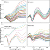 |
Fig. 1 Denoised and normalized spectra of silicate minerals, mixtures, and meteorite samples with 50 nm wavelength steps. |
3 Machine learning models
We developed two alternative machine learning models, both motivated by the limited data and the imbalanced distribution of the surface ages. These factors were meticulously addressed in the model designs. Both models take as input the reflectance spectrum and irradiation type and output the surface age in the logarithmic scale. The structure of the models is explained in detail in the following sections.
As described in Section 2.1, the interpolation was performed at fixed wavelength intervals tailored to the specific requirements of each model. For the ensemble model, a 50-nm interval was used, while the GP model employed a 34-nm interval. These intervals ensured minimal information loss while maintaining computational efficiency. The choice of these intervals was validated by comparing the results across different intervals, showing negligible loss of spectral information. The wavelength intervals also align well with the resolution of asteroid spectra typically available in the literature. Consequently, the ensemble model uses 35 input vectors corresponding to wavelengths from 550 to 2200 nm in 50-nm increments, while the GP model uses 34-nm intervals.
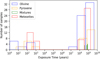 |
Fig. 2 Surface age distribution of the dataset. |
3.1 Learning and validation setup
Each of the individual models has a collection of hyperparameters that need to be selected by evaluating the model’s performance on separate validation data. To maximally efficiently use the limited data, we used k-fold cross-validation. The dataset was divided into k subsets and during the training process, the k models were trained, each using different k - 1 subsets for training and the remaining one for validation. Since each data point is used for both training and validation, this validation method makes efficient use of a limited amount of data. In validating the performance over k iterations, the method also provides a more reliable estimate of the model performance than does a single train-test split. For this study, we make the common choice of k = 10 following the recommendation of Liu & Özsu (2009).
To navigate the challenge with the imbalanced data, we implemented stratified k-fold cross-validation. A standard k-fold cross-validation could result in some folds having very few or none of the minority class samples. By stratifying the folds, each has a class distribution representing the overall dataset. This helps ensure that every fold has enough samples from each class, providing a more reliable estimate of model performance. We discretized the surface age into logarithmic ranges, each spanning an order of magnitude (e.g., 0-10, 11-100, 101-1000). Each of these ranges was then assigned a unique categorical label. This facilitates the implementation of the stratified k-fold cross-validation. The mean squared error (MSE) was used as the loss function, and mean absolute error (MAE) was used as an additional evaluation metric.
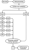 |
Fig. 3 Workflow of the ensemble model. |
3.2 Ensemble model
We combined a CNN and four tree-based machine-learning algorithms [gradient-boosting regressor (GBR), K-nearest neighbor (KNN) regressor, extra-tree regressor (ETR), and random-forest regressor (RFR)] (Breiman 2001; Friedman 2001; Geurts et al. 2006), using an ensemble method. This approach leverages the Scikit-learn VotingRegressor (Pedregosa et al. 2012) implementation, which combines the prediction of the multiple regression models to produce the final prediction (y) as a weighted average. The predictions of the individual models, yCNN, yGBR, yKNN, yETR, and yRFR, are combined using the equation,
 (8)
(8)
where wi represents the assigned weight for each model. Based on the individual model performance [measured by root-meansquare error (RMSE), and the coefficient of determination (R2) scores], the weights wCNN = 2, wGBR = 4, wKNN = 1, wETR = 5, and wRFR = 1 were assigned. The weights were chosen to maximize the overall performance of the ensemble model and were further optimized to enhance predictive accuracy. To obtain a more reliable performance estimation, we ran the model 30 times and obtained an average value for predictions. The overall model architecture is shown in Figure 3.
3.2.1 Structure of the convolutional neural network
We designed a CNN model, using the Keras library (Chollet 2015) in Python and the Keras sequential applicationprogramming interface (API) to process sequential data and learn patterns that can be used for making continuous value predictions of surface age. To increase the learning effectiveness, we combined convolutional and normalization layers. The first network takes the spectrum and the irradiation type as input parameters and processes them through a series of nonlinear operations performed by neurons. The last layer provides the surface age as its output.
The model consists of a 1D convolutional layer with 64 and 32 filters, a kernel size of 3 and 2, and ‘ReLU’ activation function, and two batch normalization layers to speed up training and stabilize the learning process. The final parameters are summarized in Table A.1. These hyperparameters were selected based on the performance of the model in validation data, using a random search over possible architecture and parameter choices (see Table A.1). An Adam optimizer was used to train the model with a learning rate of 0.001.
Comparison of the error metrics for all tree regression algorithms.
3.2.2 Structure of the tree regression models
We used four tree-regression models in the ensemble model: ETR, RFR, GBR, and KNN. Tree regressions, falling under decision tree algorithms, partition the feature space into a set of rectangles and fit a simple model in each one. They are particularly suitable for dealing with small datasets as simple as those of the model, and for interpretability. Since they do not assume any underlying distribution for data, they are suitable for small datasets with complex relationships. They can also handle missing values, and can easily provide insights into feature importance, helping researchers understand which features are most predictive of the target variable in small datasets. We trained and evaluated nine models, and selected tree regression algorithms based on RMSE ≤ 0.315 and R2 ≥ 0.9888 (see Table 2).
3.3 GP model
The GP model was implemented using the GPyTorch (Gardner et al. 2021) package for Python. We used a CNN for extracting useful features from the reflectance spectrum similar to Wilson et al. (2016) and then modeled the relationship between those features and the log-age with a GP, a nonlinear regression model. We assumed the real ages are normally distributed around the predictions, and hence we obtained a closed-form analytic expression for the posterior of the regression functions Rasmussen & Williams (2006), not requiring approximate inference. We considered the problem as a Hadamard multitask regression problem (Bonilla et al. 2007), where separate but related models are trained for each of the irradiation and mineral composition types.
Figure 4 is a visualization of the model’s architecture and Table A.2 shows a more detailed overview of some of the model components. The components of the GP model are further explained in the next sections.
The feature extractor is similar to that of Wilson et al. (2016), a deep kernel model with some structural changes such as the number and type of layers. More specifically, the feature extractor uses three layers: a convolutional layer with ReLU activation, max pooling layer, and a fully connected layer. The goal of the feature extractor is to identify the most relevant aspects of the data features in terms of predicting the target value and to give them more weight in comparison to the less important aspects. It takes the reflectance values of a data point as an input and outputs the same number of extracted features. The structure of the feature extractor, consisting of convolutional and fully connected layers with appropriate pooling for retaining the dimensionality is visible in Figure 4, and the detailed hyperparameters specifying the layers are provided in Table A.3.
A Hadamard multitask GP regression means that the model divides itself into multiple related tasks that separate different training scenarios, or in our case, data with different mineral compositions and irradiation types (Bonilla et al. 2007). The separation of the tasks is done to better capture the unique features of each different data category. By sharing information between tasks and determining inter-task correlations, the model retains the ability to benefit from inter-task similarities or dissimilarities in the data. The model takes the reflectance values as well as a task index value as input for each data point. The task index value describes the task to which the data point is assigned, based on its irradiation and composition. The model uses an index kernel to calculate a task-similarity matrix, which is used alongside the covariance function in training and prediction. The index kernel is defined by
 (9)
(9)
where a low-rank matrix B and a nonnegative vector v are learned parameters. The goal of the Hadamard multitask GP regression is to improve the model’s performance in comparison to a basic GP model with different data categories as binary features, or a model where the tasks are fully separated into independent models.
The following is a description of the model’s functionality and structure combining the different elements. The model receives reflectance values and a task index value based on the data category as input. Features are first extracted from the reflectance values using the previously described feature extractor. To apply normalization, the features are then scaled into a standardized range from −1 to 1. We use the following constant mean:
 (10)
(10)
where C is a learned constant and the Matern kernel kMatern(x1, x2) characterizes the prior assumption on the regression functions. The mean function determines the expected value of the data before taking into account the effect of the kernel (Rasmussen & Williams 2006). The kernel is responsible for describing the variations along the mean function. The Matern kernel is defined between inputs x1 and x2 by
 (11)
(11)
where Γ(ν) is the gamma function, ν is a smoothness parameter,  is the distance between x1 and x2 scaled by the length scale parameter, θ, and Kν is a modified Bessel function (Gardner et al. 2021). We used ν = 0.5 and θ = I, where I is the identity matrix. The smoothness ν of the Matern kernel describes its adaptability to the training data. The previously described multitask kernel is used to account for similarities between the different data categories. The model outputs a resulting multivariate normal distribution.
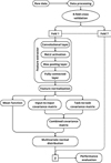 |
Fig. 4 Workflow of the GP model. |
3.3.1 GP training and optimization
Conditional on the observed data, the posterior distribution of the regression functions is available in closed form and hence requires no training. However, the accuracy of a GP model depends heavily on the hyperparameters, which here include all the parameters of the CNN feature extractor, the mean function parameter C, and the multitask function parameters B and v. Following standard practice, we optimized these parameters by maximizing the marginal log-likelihood of the observed data, using gradient-based optimization. We used the Adam optimizer with a learning rate of 0.1 and 150 iterations, which we considered sufficient in our experiments.
Besides the exact model explained above, we conducted preliminary experimentation over alternative model formulations. The selection of the GP model’s structure, components, and settings was performed by testing different options and their combinations. Examples of these include exact, approximate, deep, or multitask models, feature extractor structure and components, mean function, covariance function, feature normalization, automatic relevance determination (ARD), learning rate, and jitter, among other GP functionalities and GPyTorch settings. The chosen design was considered the best and was then fine-tuned as explained above.
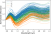 |
Fig. 5 Denoised and normalized spectra of S-, Sq-, and Q-type asteroids at 50-nm wavelength. |
4 Applying the models to asteroid spectra
After validating the models, we applied them to predict the surface age of asteroid spectra. The asteroid dataset consists of 221 reflectance spectra from S-, Sq-, and Q-type asteroids, based on data from DeMeo et al. (2009) and Binzel et al. (2019). Among the Bus-DeMeo taxonomy classes assigned are 138 S-, 43 Sq-, and 40 Q-type asteroids spanning a wavelength range of 5502200 nm, at an original resolution of 10 nm. For the ensemble model, we resampled the spectra to 50-nm intervals, and for the GP model to 35-nm intervals. We also denoised the data using a Gaussian method explained in Section 2.1 and normalized all spectra at 550 nm (see Figure 5).
As previously mentioned, the irradiation method (either H+ irradiation or laser irradiation) was included as an input parameter when training the machine-learning models. For asteroid spectra, the dominant SW process is unknown. Hence, asteroid reflectance spectra were fed into the model in two scenarios, with H+ irradiation used in one instance and laser irradiation in the other. As a result, both the ensemble and Gaussian Process (GP) models generate two outputs: one representing the surface age of the asteroid assuming solar wind dominance, and the other representing the surface age assuming micrometeorite impact dominance.
Previous studies have shown that solar wind irradiation dominates in the early stages of SW and gets saturated, after which micrometeorite impacts become more dominant (Vernazza et al. 2009; Marchi et al. 2006; Chrbolková et al. 2021; Palamakumbure et al. 2023). To determine which SW process is dominant, we first defined a saturation region where the surface is fully saturated by solar wind, based on the surface ages predicted by the model assuming solar wind dominance. S-type asteroids are considered to have mature surfaces (Vernazza et al. 2009; Binzel et al. 2010, 2019). Therefore, we assumed that their surfaces had been saturated by solar wind irradiation and applied the Huber robust regression method to fit a regression line for the S-type asteroids. Then, we plotted a saturation region corresponding to the 95% confidence interval to distinguish asteroids with saturated solar wind from those that have not reached saturation yet. Asteroids located below the lower boundary of this saturation region were classified as having unsaturated (solar wind) surfaces, and the surface age was determined assuming solar wind dominance. For the asteroids that fall within the saturation region, the surface age was determined assuming micrometeorite impact dominance (see Sections 5.2 and 6.1). This process, illustrated in Figure 6, selects the dominant SW condition.
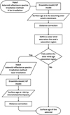 |
Fig. 6 Workflow to determine SW process. |
5 Results
5.1 Model validation
Figure 7 presents the results of the model validation. In these plots, the horizontal axis represents the true surface age in years, while the vertical axis represents the predicted surface age in years. The model was trained using the logarithmic scale. Consequently, the factor errors of two and four were calculated, corresponding to the diagonal reference lines in the plots. Each point represents the mean value of predictions over 30 iterations, while the corresponding vertical lines give the standard deviation. These diagonal lines serve as benchmarks for the accuracy of the predictions, indicating how closely the predicted values align with the true surface ages. An R2 value was calculated for both models, with the ensemble model achieving an R2 value of 0.990, and the GP model yielding a slightly higher R2 of 0.993.
Additionally, we calculated the 90th and 95th percentile factor errors to assess the distribution of prediction errors (Figure 8). These factor errors represent multiplicative uncertainties, meaning that a factor error of 2.95 indicates that the predicted value could deviate by a factor of up to 2.95, either overestimated or underestimated. In other words, a factor error of 2.95 corresponds to a deviation of up to 195% overestimation or 66% underestimation relative to the true value.
The 90th percentile factor error was 2.95 and 2.39 for the ensemble and GP models, respectively, while the 95th percentile factor error was 3.87 and 2.89. This suggests that, in 90 and 95% of cases, the predicted values fall within a range defined by these multiplicative factors. The lower factor errors for the GP model indicate its ability to minimize prediction deviations.
For a more detailed assessment, we computed the RMSE and percentile factor errors across five distinct data ranges: 1-102 years, 102−103 years, 107−108 years, 108−109 years, and 109−1010 years. These results are summarized in Table 3. Only six samples fell within the 107−108 year range, resulting in a higher RMSE value for this subset.
To estimate the lowest age limit our models are able to predict, we applied them to a set of eight fresh OC meteorite samples. As these meteorites are composed of unaltered material with no SW, the models should output the lowest possible age, close to zero. The predicted surface ages for these samples are presented in Table 4. The ensemble model has a lower limit in order of 101 years and the GP model 102 years for H+ irradiation at 1 AU. In contrast, when laser irradiation becomes the primary process, both models can accurately predict surface age down to ≈1 × 10⁸ years at 1 AU. These findings provide a useful guideline for the minimum timescales that can be reliably modeled based on the underlying irradiation mechanisms.
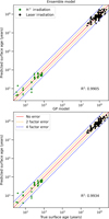 |
Fig. 7 Scatter plot of the true and predicted values after k-fold crossvalidation for both the ensemble and GP models. The red line gives the nonfactor error, the orange line the two-factor error, and the blue line the four-factor error. |
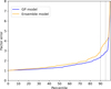 |
Fig. 8 Percentiles of the factor error between the true and predicted values of the ensemble and the GP models. The dashed lines indicate the factor error at the 90th and 95th percentiles. GP = Gaussian process. |
5.2 Evaluation of asteroid spectra
The predicted and the corrected surface age for these asteroids are provided in Table B.1 available in CDS database (see Section for details). For the ensemble model, the surface ages ranged from 1.12 × 10² to 5.29 × 10³ years for H+ irradiation at 1 AU and from 1.33 × 10⁸ to 1.67 × 10⁹ years for laser irradiation at 1 AU. In the GP model, these intervals were similar 1.71 × 10²−9.51 × 10³ years for H+ irradiation and 2.48 × 10⁸−1.77 × 10⁹ years for laser irradiation at 1 AU. In the following text, we refer to these ages at 1 AU H+ age and 1 AU laser age, respectively.
The models’ output is valid for solar wind and dust conditions at 1 AU. Hence, the predicted surface age needs to be adjusted for given asteroid semimajor axis. We applied this correction for distances ranging from 0.8 to 3 AU, where the majority of S-, Sq-, and Q-type asteroids are located. Ages for micrometeorite impacts were corrected using Equations (4)-(7) and micrometeorite velocity and flux values were adopted from a model developed by Jehn (2000). The solar wind irradiation was corrected for decreasing the proton flux by the square of the distance from the Sun (Schwenn 2000) (as in the Equation (4)). In the case of the ensemble model, the corrected surface ages ranged from 2.16 × 10² to 3.57 × 10⁴ years for solar wind irradiation and 9.46 × 10⁷ to 4.89 × 10⁹ years for micrometeorite impacts. In the case of the GP model, the ages ranged from 1.64 × 10² to 5.47 × 10⁴ years for solar wind irradiation and from 1.09 × 10⁸ to 5.30 × 10⁹ years for micrometeorite impacts (Figure 9). In the following text, we refer to these as distance-corrected H+ and distance-corrected laser age, respectively.
The mean surface age value of each taxonomy 1 AU H+ ages [subplots (a) and (c)] and distance-corrected H+ ages [subplots (b) and (c)] are plotted in Figure 9 where the horizontal axis represents the semimajor axis in AU, while the vertical axis represents the distance-corrected H+ ages in years. The lower H+ irradiation limit at 1 AU ≈ 102 years is in line with the model sensitivity boundary as determined on fresh meteorites. Thus, asteroids with this predicted surface age (mostly Q-types) can be assumed to have a fresh surface with minimum SW. The upper value ≈104 years is seen for S-type asteroids and corresponds to a saturation limit of the SW solar wind component above which spectral changes no longer evolve significantly (red region in Figure 9). Using the method illustrated in Figure 6, the ensemble model identified 31 asteroids with fresh surfaces, while the GP model identified 47.
After separating the fresh and matured asteroids, Figure 10 plots the surface age against the semimajor axis for the asteroids below the solar wind saturation region with distance-corrected H+ age and for the asteroids in the solar wind saturation region with distance-corrected laser age. The horizontal axis represents the semimajor axis in AU, while the vertical axis shows the predicted surface age in years. Each point represents the mean surface age across 30 iterations, with vertical lines indicating the standard deviation, and the points are color-coded by taxonomy. Even without distance correction [subplots (a) and (c)], a clear trend emerges, with Q-type asteroids exhibiting younger surface ages than the S-types. Once the surface ages are corrected for distance [subplots (b) and (d)], this trend persists.
In Figure 10, we observe that asteroids located in the main Asteroid Belt exhibit reduced surface exposure ages. According to our model, this region is characterized by a micrometeoroid impact-dominated environment, which plays a significant role in surface processing. At greater heliocentric distances close to 3 AU, the average impact velocity increases (Jehn 2000), resulting in higher energy deposition per impact event. This leads to a shorter surface age.
Percentile factor error and RMSE for the two models.
Predicted values for the fresh meteorite samples.
5.2.1 Trends in asteroid surface age estimate pertaining to taxonomy class, size, and semimajor axis
We applied the models to identify trends based on the surface ages among the asteroids. In Figure 11, we plotted the distribution of the surface age with the diameter. The horizontal axis represents the diameter of the asteroid in km, while the vertical axis represents the predicted surface age in years. The vertical dashed black line represents the 5-km diameter. Each point represents the mean value of predictions over 30 iterations, and the corresponding vertical lines give the standard deviation. We color-coded the points according to their taxonomy and used different symbols for asteroids located in the region 0-2 AU and >2 AU.
Figure 12 presents the percentile distribution of surface age for asteroid size groups: 0.2-5 km, 5-20 km, 20-50 km, 50-100 km, and 100-1000 km. In the plot, the horizontal axis represents the percentile, while the vertical axis represents the predicted surface age in years corrected for the distance. The vertical dashed black line gives the 90th percentile, and the horizontal lines give the corresponding predicted surface age in years for each size group. The ensemble model has resulted in estimates that 90% of the asteroids in the 0.2-5 km size group have surface ages in the ranges of 2 × 10²−3.5 × 10⁹ years. For the other size groups (5-1000 km), surface ages predominantly fall within 3 × 10⁸−2.5 × 10⁹ years. In comparison, the GP model produced similar surface age estimates, with the 0.2-5 km group ranging from 1 × 10²−3 × 10⁹ years, and the remaining groups (5-1000 km) ranging from 1 × 10⁸−2.5 × 10⁹ years. In both models, there was a clear transition from a relatively younger surface age for asteroids 0.2-5 km in diameter to an older surface age for larger asteroids.
Asteroids with <5 km diameter show a wide range of surface age. Notably, Q-type asteroids in our dataset falls within this size range, and most of them have been identified to have young surface ages. Both smaller and larger S- and Sq-type asteroids dominate at older surface ages.
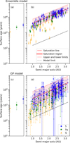 |
Fig. 9 Surface ages for S-, Sq-, and Q-type asteroids assuming H+ irradiation (solar wind) without (a, c) and with (b, d) distance correction. GP = Gaussian process, AU = astronomical unit. |
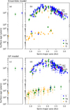 |
Fig. 10 Surface ages for S-, Sq-, and Q-type asteroids plotted against the semimajor axis. (a), (c): Predicted surface age without the distance correction. (b), (d): Predicted surface age with the distance correction. Red dots: Refer to Table 5. |
6 Discussion
6.1 Model performance with asteroid data
In comparing the predictive performance of the ensemble and GP models in the asteroid dataset, notable differences in accuracy and variability emerged. Despite the better performance of the GP model during model validation with a lower standard deviation and higher R2, its predictions for the asteroid data demonstrated considerably higher standard deviations. The higher standard deviations of the GP results were caused by the nature of the interactions governing how GP and its components function. In general, GP tries to find the most probable function that fits the training data (Rasmussen & Williams 2006). By that nature, it is prone to assigning high weight to individual data points in cases where the data are sparse. This can lead to high variance as the model fits the data. This variance can be controlled, (e.g., with different mean functions and kernels). In contrast, the ensemble model has a more conservative degree of variance, which makes sense since it is a combination of multiple models. While the GP model remains a valuable tool for understanding complex relationships, its higher variability may limit its utility in cases where low-uncertainty predictions are crucial, such as in the precise dating of asteroid surfaces.
However, the predicted values at 1 AU slightly fall outside the training data between 103−104 years. Predicted values for this range could be influenced by data just below the 103-year mark. The two models might infer that the underlying pattern in the training data extends into the gap, producing plausible but unverified predictions. In the ensemble model, the combined behavior of its components can lead to minor deviations outside the training range due to differences in individual model predictions and their aggregation (Shi et al. 2024). Similarly, GP models, being inherently probabilistic, are capable of interpolating values in regions without direct training data, leveraging their assumptions about smoothness and continuity (Rasmussen & Williams 2006; Liu & Özsu 2009; Roberts et al. 2013).
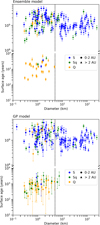 |
Fig. 11 Surface age distribution for S-, Sq-, and Q-type asteroids plotted against the diameter of the asteroids. GP = Gaussian process, AU = Astronomical unit |
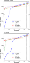 |
Fig. 12 Percentile distribution of surface age for asteroid size groups: 0-5 km, 5-20 km, 20-50 km, 50-100 km, and 100-1000 km. The dashed black line indicates the 90th percentile, and the corresponding surface age for each group is given by the horizontal dashed lines. |
6.2 S-, Sq-, and Q-type asteroids
In the two models, we observed a general tendency between the S-, Sq-, and Q-type (S-Q continuum), which is consistent with previous studies (Vernazza et al. 2009; Binzel et al. 2010, 2019). These studies suggest that spectra of Q- and S-type asteroids deviate due to SW effects, with Q-type asteroids being fresher and S-types more mature. As noted by Marchi et al. (2006), Chrbolková et al. (2021), and Palamakumbure et al. (2023), solar wind is highly effective during the initial stages of SW but begins to saturate within 103−104 years at 1 AU. Beyond this saturation point, the effects of micrometeorite impacts become more significant. Most of the predicted surface ages for Q-type asteroids were below the saturation threshold (see Figure 9), suggesting that they have not reached saturation with respect to solar wind exposure. Most of the Sq-type asteroids in our dataset fell within the saturation region, suggesting that the micrometeorite impact SW starts to dominate within these asteroids. The derived surface age clouds of the S-, Sq-, and Q-type asteroids are not fully separated. The overlap is likely due to the transitional nature of these asteroid spectral types manifesting the continuous evolution of SW.
6.3 Size and surface age
In our two models, we observed a clear tendency for surface age to increase with asteroid size, a pattern consistent with findings from previous studies (Gaffey et al. 1993; Dandy et al. 2003; Vernazza et al. 2009; Thomas et al. 2012; Carry et al. 2016; Binzel et al. 2019; Sergeyev et al. 2023). This tendency can be explained by the dynamic and collisional evolution of the asteroid population. Notably, in the two models, a distinct transition occurs at an approximate diameter of 5 km, where the asteroid’s surface shifts from relatively fresh to more mature (see Figure 11). This transition is also seen in asteroid semimajor axis statistics with <5 km asteroids being predominantly Q-types and located mostly in the 0-2 AU region, while larger S-types have semimajor axis mostly >2 AU.
In both our models, we observed that in the region 0-2 AU, where smaller asteroids (diameters <5 km) predominate, there is a clear transition from Q-type to S-type asteroids as they age. Furthermore, most Q-type asteroids at 0-2 AU also exhibit the lowest distance-corrected H ages below 104 years. This is consistent with observations by Vernazza et al. (2008), who suggested that Q-type asteroids among the Near-Earth Asteroids (NEAs) retain their fresh surfaces by frequent rejuvenation. A similar tendency was observed by Binzel et al. (2019) for S-, Sq-, and Q-type NEAs and they identified 5 km as the critical size for completing the transition from Q-type to S-type. Sergeyev et al. (2023), who studies the spectral slope variations in S-, Sq-, and Q-type NEAs reported that the spectral slope in the visible range, indicative of SW, remains relatively constant for S-type asteroids in the 1-5 km range, but increases for larger asteroids. This implies that asteroids in the 1-5 km range do have generally fresher surfaces than the larger asteroids. Their observation of relatively fresh surfaces on smaller asteroids is consistent with the rejuvenation model through thermal fatigue by Graves et al. (2019). From the same Graves et al. (2019) model larger asteroids have more stable surfaces due to the combination of high thermal inertia, stronger gravitational binding (less surface material shedding), and more stable temperature fluctuations resulting in less effective thermal fatigue.
The size transition is more pronounced in the Main Asteroid Belt population than in the NEA region (0-2 AU). This finding aligns with observations by Thomas et al. (2012), who noted a similar tendency in the small Koronis family asteroids in the asteroid belt. In their study, asteroids smaller than 4 km demonstrated a transition from fresh Q-type surfaces to weathered S-type surfaces. Our results support this observation, suggesting that smaller Q-type asteroids tend to have younger surface ages, consistent with the surface evolution patterns identified in the Koronis family.
Smaller asteroids are also more likely to be products of collisional fragmentation or disruption of larger parent bodies (O’Brien & Greenberg 2005), explaining the prevalence of younger surface age (<108 years) for asteroids in the 05 km diameter range. Nevertheless, the dynamic evolution of smaller asteroids is heavily influenced by effects such as the Yarkovsky-O’Keefe-Radzievskii-Paddack (YORP) effect and planetary encounters (Bonanno 2000; DeMeo et al. 2023). The YORP effect, which causes a slow drift in asteroid orbits due to anisotropic thermal radiation, is more pronounced for smaller bodies because of their higher surface-area-to-mass ratio. Consequently, these asteroids tend to have younger surface ages as they are more likely to have been disrupted or stripped of their surface material at relatively recent ages. A study conducted by Graves et al. (2018) shows that YORP spin-up and structural failure are efficient mechanisms for resurfacing small asteroids. According to their model, the YORP-induced resurfacing is relatively more efficient than other processes that specifically impact small asteroids. Combined, these resurfacing processes support our observation of lower predicted surface ages of small asteroids.
In contrast, larger objects have extended collisional lifespans, due to their lower probability of catastrophic disruption, slower dynamic evolution, and reduced susceptibility to fragmentation, resulting in longer surface ages (Chapman 2004; Richardson et al. 2005). This is consistent with the surface ages observed in >109 years in our models.
6.4 Comparison of our semimajor with absolute surface age estimates derived using other methods
The absolute surface ages of asteroids listed in Table 5 - and shown as red dots in Figure 10 - were determined using our models. When comparing our results with the dynamic ages reported in previous studies (Marzari et al. 1995; Bottke et al. 2001; Nesvorny et al. 2003; Spoto et al. 2015), our estimates generally align with those of Spoto et al. (2015), with the exception of Massalia and Jitka. Spoto et al. (2015) used the Yarkovsky effect and inverse slopes and predicted the ages for 37 collisional families. This method extracts asteroid family ages from the observed slope of a V-shaped distribution of family members in orbital element space. It also minimized systematic errors that could arise from relatively unknown thermal properties. However, the model was limited by the availability of data for Main Belt asteroids; reliance on extrapolated values introduces uncertainties.
However, for asteroids with ages of approximately 100 million years and younger at 1 AU, our models tend to overestimate the surface ages due to the gap in the data. Evidence from fresh meteorite samples indicated that, at 1 AU, the minimum reliable surface age in a micrometeorite-dominated impact environment is 1 × 10⁸ years. This threshold increases to 3 × 10⁸ years between 2.4 and 2.7 AU. Therefore, the ages of Massalia and Jitka reported by Spoto et al. (2015) fall outside the reliable range of the performance of our models, and their ages may have been overestimated as a result.
In contrast to our findings, other studies have employed different approaches to determine asteroid ages. For instance, Marzari et al. (1995) determined the ages of the Themis, Koronis, and Eos families by developing a collisional model for the evolution of the size-frequency distribution (SFD) of asteroid families over time. The modeling provided a quantitative framework for estimating asteroid ages based on observable SFD, contributing to a more systematic understanding of asteroid family evolution. Their findings support the notion that prominent asteroid families are significantly older than previously believed. However, in the case of the Eos family, the collision code failed to generate a reasonable match with the SFD observed, indicating that the model may not be universally applicable to all asteroid families.
Nesvorný et al. (2003) and Bottke et al. (2001) estimated asteroid family ages by modeling orbital spreading from the Yarkovsky effect, comparing observed orbital distributions with model predictions. While effective, this method is sensitive to uncertainties in physical properties and initial conditions. Marsset et al. (2024) provided spectroscopic and dynamical evidence that the Massalia family is up to 500 My old using a modified SWIFT integrator, and modeling the orbital evolution of approximately 1000 Massalia fragments over 50 Myr, accounting for thermal forces and spin dynamics. However, our models give an overestimation of 900 My age for Massalia.
All these studies have determined surface ages based on orbital parameters, which primarily reflect the time since the breakup event. In a break-up event, a freshly exposed material mixes with the mature surface material. Thus, the resurfacing in terms of SW may not be complete, and the resulting collisional fragments may retain a portion of the spectrally mature material mixed together with the freshly exposed interior, resulting in a higher age derived from the asteroid spectra.
A key limitation of the study lies in the data gap between 103 years and 107 years caused by the short timescale simulations through H+ (102−103) and long timescales through laser (108−109) with no age overlap between these two methods (see Figure 2), resulting in reduced predictive power in the intermediate region. This gap represents a region where neither model can offer reliable predictions, a fact that must be clearly acknowledged in applications of these models and demonstrates the overall limitation of currently existing laboratory SW simulation data. However, this can be improved as more data becomes available to bridge the current gap. The models in this study also assumed a direct correlation between surface reflectance and surface age, which may vary based on the asteroid’s size, composition, and location. These differing assumptions can lead to significant discrepancies in estimating absolute age. These models are also highly reliant on interplanetary environmental conditions derived from flux models. Despite the absolute surface age, the models show more promise in making a relative comparison of surface ages between asteroids. The application of the ensemble and GP models to the asteroid dataset yielded predictions that aligned with general trends observed in previous studies, as discussed in the previous sections. Hence, it is safe to say that these models provide a promising avenue for future research on surface age prediction. Future models will be utilized to determine the surface age variation of a single asteroid body and to identify asteroid families.
List of asteroids with ages predicted by our model and by previous studies.
7 Conclusion
This study demonstrates that both the ensemble and GP models can effectively distinguish between fresh and mature asteroid surfaces based on SW features in the reflectance spectra, within the data range on which they were trained. While the training data followed a bimodal age distribution, the model was not explicitly provided with asteroid taxonomy or size as input parameters. Yet, the results reveal a clear transition from Q-type to S-type asteroids, with the majority of younger surfaces predominantly classified as Q-type, and the majority of S-types associated with mature surfaces. Additionally, no asteroid larger than 5 km was assigned young ages, further supporting the model’s ability to capture meaningful physical trends. These findings indicate that the model learned spectral features that correlate with both surface aging and taxonomic evolution, rather than merely reproducing the bimodal nature of the training data. The consistency of these trends, despite the absence of explicit taxonomy or size input, suggests that the model identifies real evolutionary processes rather than statistical artifacts.
However, the GP model’s higher variability in predictions for asteroids highlights the need for caution when low-uncertainty predictions are required. A significant limitation of this study is the data gap between 103 and 107 equivalent years of surface age at 1 AU, reducing the models’ predictive power in this intermediate range. While the two models perform well within the available training ranges, extrapolation into this gap should be avoided. The smaller sample size in certain surface age ranges also contributes to uncertainty in predictions, particularly for younger asteroids.
Furthermore, future improvements, such as filling the current data gaps and incorporating more diverse datasets, will enhance their precision. These models have significant potential for future applications, such as determining the surface age for individual asteroids and identifying asteroid families, offering valuable tools for advancing our understanding of asteroid evolution and SW processes.
Acknowledgements
This work was supported by the Doctoral program of the University of Helsinki and the Czech-German common grant, funded by the Czech Science Foundation under the project 23 07633K and by the Deutsche Forschungsgemeinschaft under the project BE 5771/3-1 (eBer-23 13412) and by the institutional support RVO 67985831 of the Institute of Geology of the Czech Academy of Sciences. We would like to thank Francesca DeMeo and Richard Binzel for providing us with the dataset on the asteroid spectra. We utilized data stored in the RELAB Spectral Database operated by Brown University and the C-Tape database operated by the University of Winnipeg. Taxonomic type results presented in this work were determined, in whole or in part, using a Bus-DeMeo Taxonomy Classification Web tool by Stephen M. Slivan, developed at MIT with the support of National Science Foundation Grant 0506716 and NASA Grant NAG5-12355. We also would like to extend our thanks to Rosario Brunetto and Zuzana Kanuchová for providing laboratory reflectance data. This research has made use of NASA’s SmallBody Database Lookup and the AsteroidFamiliesPortal (Bojan Novakovic, David Vokrouhlický, Federica Spoto and David Nesvorny: Asteroid Families: properties, recent advances and future opportunities 2022, Celest Mech Dyn Astro, 134, id. 34). This research has made use of NASA’s Astrophysics Data System Bibliographic Services.
Data availability
The Python scripts, and datasets including all the sample spectra and composition information we used in this study, together with metadata, can be downloaded from the GitHub repository at https://github.com/Lakshika1990/Asteroid_surface_age_prediction and from Zenodo repository (Palamakumbure et al. 2025). Table B.1 is available at the CDS via anonymous ftp to cdsarc.cds.unistra.fr (130.79.128.5) or via https://cdsarc.cds.unistra.fr/viz-bin/cat/J/A+A/699/A175
Appendix A Hyper parameters of the machine learning models
Hyperparameters for the CNN model.
Overview of the GP model’s components.
Hyperparameters for the GP model’s feature extractor.
References
- Bennett, C. J., Pirim, C., & Orlando, T. M. 2013, Chem. Rev., 113, 9086 [NASA ADS] [CrossRef] [Google Scholar]
- Binzel, R. P., Morbidelli, A., Merouane, S., et al. 2010, Nature, 463, 331 [NASA ADS] [CrossRef] [Google Scholar]
- Binzel, R. P., DeMeo, F. E., Turtelboom, E. V., et al. 2019, Icarus, 324, 41 [Google Scholar]
- Bonanno, C. 2000, A&A, 360, 411 [NASA ADS] [Google Scholar]
- Bonilla, E. V., Chai, K. M. A., & Williams, C. K. I. 2007, in Advances in Neural Information Processing Systems (Cambridge: MIT Press), 20 [Google Scholar]
- Bottke, W. F., Vokrouhlicky, D., Broz, M., Nesvorny, D., & Morbidelli, A. 2001, Science, 294, 1693 [NASA ADS] [CrossRef] [Google Scholar]
- Breiman, L. 2001, Mach. Learn, 45, 5 [CrossRef] [Google Scholar]
- Brunetto, R., Romano, F., Blanco, A., et al. 2006, Icarus, 180, 546 [NASA ADS] [CrossRef] [Google Scholar]
- Brunetto, R., Lantz, C., Ledu, D., et al. 2014, Icarus, 237, 278 [NASA ADS] [CrossRef] [Google Scholar]
- Carry, B., Solano, E., Eggl, S., & DeMeo, F. 2016, Icarus, 268, 340 [CrossRef] [Google Scholar]
- Chapman, C. R. 1996, Meteor. Planet. Sci., 31, 699 [NASA ADS] [CrossRef] [Google Scholar]
- Chapman, C. R. 2004, Ann. Rev. Earth Planet. Sci., 32, 539 [Google Scholar]
- Chapman, C., Enke, B., Merline, W., et al. 2007, Icarus, 191, 323 [Google Scholar]
- Chollet, F. 2015, Keras, https://github.com/fchollet/keras [Google Scholar]
- Chrbolková, K., Brunetto, R., Durech, J., et al. 2021, A&A, 654, A143 [NASA ADS] [CrossRef] [EDP Sciences] [Google Scholar]
- Dandy, C., Fitzsimmons, A., & Collander-Brown, S. 2003, Icarus, 163, 363 [NASA ADS] [CrossRef] [Google Scholar]
- DeMeo, F. E., Binzel, R. P., Slivan, S. M., & Bus, S. J. 2009, Icarus, 202, 160 [Google Scholar]
- DeMeo, F. E., Marsset, M., Polishook, D., et al. 2023, Icarus, 389, 115264 [NASA ADS] [CrossRef] [Google Scholar]
- Divine, N., Grün, E., & Staubach, P. 1993, in Space Debris, ed. W. Flury, 245 [Google Scholar]
- Fazio, A., Harries, D., Matthäus, G., et al. 2018, Icarus, 299, 240 [CrossRef] [Google Scholar]
- Friedman, J. H. 2001, Annal. Stat., 29, 1189 [CrossRef] [Google Scholar]
- Gaffey, M. J., Bell, J. F., Brown, R. H., et al. 1993, Lunar Planet. Sci. Conf., 515 [Google Scholar]
- Gardner, J. R., Pleiss, G., Bindel, D., Weinberger, K. Q., & Wilson, A. G. 2021, arXiv e-prints [arXiv:1809.11165] [Google Scholar]
- Geurts, P., Ernst, D., & Wehenkel, L. 2006, Mach. Learn., 63, 3 [Google Scholar]
- Graves, K. J., Minton, D. A., Hirabayashi, M., DeMeo, F. E., & Carry, B. 2018, Icarus, 304, 162 [CrossRef] [Google Scholar]
- Graves, K. J., Minton, D. A., Molaro, J. L., & Hirabayashi, M. 2019, Icarus, 322, 1 [NASA ADS] [CrossRef] [Google Scholar]
- Grun, E., Fechtig, H., Hanner, M. S., et al. 1991, Astrophys. Space Sci. Lib., 173, 21 [Google Scholar]
- Han, H.-J., Lu, X.-P., Jiang, T., et al. 2021, Res. Astron. Astrophys., 21, 127 [Google Scholar]
- Hasegawa, S., Hiroi, T., Ohtsuka, K., et al. 2019, PASJ, 71, 5 [Google Scholar]
- Hiroi, T., & Sasaki, S. 2001, Nature, 36, 1587 [Google Scholar]
- Hiroi, T., Abe, M., Kitazato, K., et al. 2006, Nature, 443, 56 [CrossRef] [Google Scholar]
- Hiroi, T., & Sasaki, S. 2012, in Asteroids, Comets, Meteors Conference (Niigata, Japan), 6109 [Google Scholar]
- Ishiguro, M., Hiroi, T., Tholen, D. J., et al. 2007, Meteor. Planet. Sci., 42, 1791 [NASA ADS] [CrossRef] [Google Scholar]
- Jedicke, R., & Nesvorny, D. W. 2004, Nature, 429, 275 [NASA ADS] [CrossRef] [Google Scholar]
- Jehn, R. 2000, Planet. Space Sci., 48, 1429 [Google Scholar]
- Kaluna, H. M., Ishii, H. A., Bradley, J. P., Gillis-Davis, J. J., & Lucey, P. G. 2017, Icarus, 292, 245 [Google Scholar]
- Kanuchova, Z., Brunetto, R., Fulvio, D., & Strazzulla, G. 2015, Eur. Planet. Sci. Cong., 36 [Google Scholar]
- Koga, S. C., Sugita, S., Kamata, S., et al. 2018, Icarus, 299, 386 [CrossRef] [Google Scholar]
- Korda, D., Penttilä, A., Klami, A., & Kohout, T. 2023a, A&A, 669, A101 [NASA ADS] [CrossRef] [EDP Sciences] [Google Scholar]
- Korda, D., Kohout, T., Flanderová, K., Vincent, J.-B., & Penttilä, A. 2023b, A&A, 675, A50 [NASA ADS] [CrossRef] [EDP Sciences] [Google Scholar]
- Kurahashi, E., Yamanaka, C., Nakamura, K., & Sasaki, S. 2002, Earth Planet Space, 54, e5 [Google Scholar]
- Liu, L., & Özsu, M. T. 2009, Encyclopedia of Database Systems (New York, NY, USA: Springer), 6 [Google Scholar]
- Marchi, S., Brunetto, R., Magrin, S., Lazzarin, M., & Gandolfi, D. 2005, A&A, 443, 769 [NASA ADS] [CrossRef] [EDP Sciences] [Google Scholar]
- Marchi, S., Paolicchi, P., Lazzarin, M., & Magrin, S. 2006, AJ, 131, 1138 [NASA ADS] [CrossRef] [Google Scholar]
- Marsset, M., Grun, P. and Broz, M., Thomas, C. A., et al. 2024, Nature, 634, 561 [Google Scholar]
- Marzari, F., Davis, D., & Vanzani, V. 1995, Icarus, 113, 168 [NASA ADS] [CrossRef] [Google Scholar]
- Moroz, L. V., Fisenko, A. V., Semjonova, L. F., Pieters, C. M., & Korotaeva, N. N. 1996, Icarus, 122, 366 [NASA ADS] [CrossRef] [Google Scholar]
- Nesvorny, D., Bottke, W. F., Levison, H. F., & Dones, L. 2003, ApJ, 591, 486 [CrossRef] [Google Scholar]
- Nesvorny, D., Jedicke, R., Whiteley, R. J., & Ivezic, $Z. 2005, Icarus, 173, 132 [CrossRef] [Google Scholar]
- Noble, S. K., Pieters, C. M., Taylor, L. A., et al. 2001, Meteor. Planet. Sci., 36, 31 [NASA ADS] [CrossRef] [Google Scholar]
- O’Brien, D. P., & Greenberg, R. 2005, Icarus, 178, 179 [CrossRef] [Google Scholar]
- Palamakumbure, L., Mizohata, K., Flanderová, K., et al. 2023, Planet. Sci. J., 4, 72 [Google Scholar]
- Palamakumbure, L., Syrjänen, S. A. I., Korda, D., Kohout, T., & Klami, A. 2025, https://doi.org/10.5281/zenodo.15489128 [Google Scholar]
- Pedregosa, F., Varoquaux, G., Gramfort, A., et al. 2012, Scikit-learn: Machine Learning in Python, https://scikit-learn.org/stable/modules/generated/sklearn.ensemble.VotingRegressor.html [Google Scholar]
- Pieters, C. M., & Noble, S. K. 2016, J. Geophys. Res. Planets, 121, 1865 [CrossRef] [Google Scholar]
- Pieters, C. M., Taylor, L. A., Noble, S. K., et al. 2000, Meteor. Planet. Sci., 35, 1101 [NASA ADS] [CrossRef] [Google Scholar]
- Rasmussen, C. E., & Williams, C. K. I. 2006, Gaussian Process for Machine Learning (Cambridge: The MIT Press) [Google Scholar]
- Richardson, J. E., Melosh, H. J., Greenberg, R. J., & O’Brien, D. P. 2005, Icarus, 179, 325 [NASA ADS] [CrossRef] [Google Scholar]
- Roberts, S., Osborne, M., Ebden, M., et al. 2013, Phil. Trans. R. Soc. A Math. Phys. Eng. Sci., 371, 20110550 [Google Scholar]
- Sasaki, S., Kurahashi, E., Yamanaka, C., & Nakamura, K. 2003, Adv. Space Res., 31, 2537 [Google Scholar]
- Schwenn, R. 2000, in Encyclopedia of Astronomy and Astrophysics (Boca Raton: CRC Press), ed. P. Murdin, 2301 [Google Scholar]
- Sergeyev, A. V., Carry, B., Marsset, M., et al. 2023, A&A, 679, A148 [NASA ADS] [CrossRef] [EDP Sciences] [Google Scholar]
- Shi, S., Chen, R., Wang, P., et al. 2024, Environ. Sci. Technol, 58, 22 [Google Scholar]
- Shkuratov, Y., Starukhina, L., Hoffmann, H., & Arnold, G. 1999, Icarus, 137, 235 [Google Scholar]
- Spoto, F., Milani, A., & Kne$zevi$c, Z. 2015, Icarus, 257, 275 [NASA ADS] [CrossRef] [Google Scholar]
- Strazzulla, G., Dotto, E., Binzel, R., et al. 2005, Icarus, 174, 31 [CrossRef] [Google Scholar]
- Thomas, C. A., Trilling, D. E., & Rivkin, A. S. 2012, Icarus, 219, 505 [NASA ADS] [CrossRef] [Google Scholar]
- Vernazza, P., Binzel, R. P., Rossi, A., Fulchignoni, M., & Birlan, M. 2009, Nature, 458, 993 [NASA ADS] [CrossRef] [Google Scholar]
- Vernazza, P., Binzel, R. P., Thomas, C. A., et al. 2008, Nature, 454, 858 [NASA ADS] [CrossRef] [Google Scholar]
- Wang, P., Cloutis, E., Zhang, Q., & Wu, Y. 2022, J. Geophys. Res. Planets, 127, 12 [Google Scholar]
- Willman, M., & Jedicke, R. 2011, Icarus, 211, 504 [Google Scholar]
- Willman, M., Jedicke, R., Nesvorny, D., Vokrouhlicky, D., & Mothé-Diniz, T. 2008, Icarus, 195, 663 [Google Scholar]
- Willman, M., Jedicke, R., Moskovitz, N., et al. 2010, Icarus, 208, 758 [Google Scholar]
- Wilson, A. G., Hu, Z., Salakhutdinov, R., & Xing, E. P. 2016, Proc. Mach. Learn. Res., 51, 370 [Google Scholar]
- Yamada, M., Sasaki, S., Nagahara, H., et al. 1999, Earth Planets Space, 51, 1255 [NASA ADS] [CrossRef] [Google Scholar]
- Yang, Y., Zhang, H., Wang, Z., et al. 2016, A&A, 597, L4 [Google Scholar]
- Zhang, P., Tai, K., Li, Y., et al. 2022, A&A, 659, A78 [NASA ADS] [CrossRef] [EDP Sciences] [Google Scholar]
- Zhuang, Y., Zhang, H., Ma, P., et al. 2023, Icarus, 391, 14 [Google Scholar]
All Tables
All Figures
|
Fig. 1 Denoised and normalized spectra of silicate minerals, mixtures, and meteorite samples with 50 nm wavelength steps. |
| In the text | |
|
Fig. 2 Surface age distribution of the dataset. |
| In the text | |
|
Fig. 3 Workflow of the ensemble model. |
| In the text | |
|
Fig. 4 Workflow of the GP model. |
| In the text | |
|
Fig. 5 Denoised and normalized spectra of S-, Sq-, and Q-type asteroids at 50-nm wavelength. |
| In the text | |
|
Fig. 6 Workflow to determine SW process. |
| In the text | |
|
Fig. 7 Scatter plot of the true and predicted values after k-fold crossvalidation for both the ensemble and GP models. The red line gives the nonfactor error, the orange line the two-factor error, and the blue line the four-factor error. |
| In the text | |
|
Fig. 8 Percentiles of the factor error between the true and predicted values of the ensemble and the GP models. The dashed lines indicate the factor error at the 90th and 95th percentiles. GP = Gaussian process. |
| In the text | |
|
Fig. 9 Surface ages for S-, Sq-, and Q-type asteroids assuming H+ irradiation (solar wind) without (a, c) and with (b, d) distance correction. GP = Gaussian process, AU = astronomical unit. |
| In the text | |
|
Fig. 10 Surface ages for S-, Sq-, and Q-type asteroids plotted against the semimajor axis. (a), (c): Predicted surface age without the distance correction. (b), (d): Predicted surface age with the distance correction. Red dots: Refer to Table 5. |
| In the text | |
|
Fig. 11 Surface age distribution for S-, Sq-, and Q-type asteroids plotted against the diameter of the asteroids. GP = Gaussian process, AU = Astronomical unit |
| In the text | |
|
Fig. 12 Percentile distribution of surface age for asteroid size groups: 0-5 km, 5-20 km, 20-50 km, 50-100 km, and 100-1000 km. The dashed black line indicates the 90th percentile, and the corresponding surface age for each group is given by the horizontal dashed lines. |
| In the text | |
Current usage metrics show cumulative count of Article Views (full-text article views including HTML views, PDF and ePub downloads, according to the available data) and Abstracts Views on Vision4Press platform.
Data correspond to usage on the plateform after 2015. The current usage metrics is available 48-96 hours after online publication and is updated daily on week days.
Initial download of the metrics may take a while.