| Issue |
A&A
Volume 698, June 2025
|
|
|---|---|---|
| Article Number | A149 | |
| Number of page(s) | 10 | |
| Section | Planets, planetary systems, and small bodies | |
| DOI | https://doi.org/10.1051/0004-6361/202554398 | |
| Published online | 13 June 2025 | |
Noble gas depletion on Titan: Clathrate sequestration during the open ocean phase
1
Aix-Marseille Université, CNRS, CNES, Institut Origines, LAM,
Marseille,
France
2
Institut Universitaire de France (IUF),
France
3
Aix-Marseille Université, CNRS, Institut Origines, PIIM,
Marseille,
France
4
University of Science and Technology of Hanoi (USTH),
Hanoi,
Vietnam
★ Corresponding author: This email address is being protected from spambots. You need JavaScript enabled to view it.
Received:
6
March
2025
Accepted:
29
April
2025
Abstract
A plausible explanation for the absence of primordial argon, krypton, and xenon in Titan’s current atmosphere is that these gases were sequestered in clathrate hydrates during Titan’s “open-ocean” phase. We examine how clathrate hydrate formation at Titan’s ocean surface in its early history may have contributed to noble gas depletion in the primordial atmosphere. Starting with vapor-liquid equilibrium modeling between water and volatiles, we used a statistical thermodynamic model to determine the clathrate hydrate crust thickness needed to deplete the primordial atmosphere of noble gases. Our computations suggest that if Titan’s volatile budget was delivered by icy planetesimals with a comet-like composition, its primordial atmosphere should be rich in CO2 and CH4, with NH3 largely retained in water as ions. We show that at 273.15 K, a clathrate crust tens of kilometers thick would deplete the primordial atmosphere of xenon and krypton. The lack of primordial argon in Titan’s atmosphere may result from the partial de-volatilization of its accreted materials.
Key words: planets and satellites: atmospheres / planets and satellites: composition / planets and satellites: individual: Titan
© The Authors 2025
 Open Access article, published by EDP Sciences, under the terms of the Creative Commons Attribution License (https://creativecommons.org/licenses/by/4.0), which permits unrestricted use, distribution, and reproduction in any medium, provided the original work is properly cited.
This article is published in open access under the Subscribe to Open model. This email address is being protected from spambots. You need JavaScript enabled to view it. to support open access publication.
1 Introduction
A notable feature of Titan’s atmosphere is the absence of heavy noble gases except argon, as revealed by the Gas Chromatograph Mass Spectrometer (GCMS) aboard the Huygens probe during its descent to the surface in January 2005. The GCMS detected argon in two forms: primordial 36Ar and radiogenic 40Ar, a decay product of 40K. However, other primordial noble gases, including 38Ar, krypton (Kr), and xenon (Xe), were not detected, with GCMS placing upper limits on their atmospheric mole fractions of <10−8 (Niemann et al. 2005, 2010).
Titan is believed to have formed from a mixture of ices, silicates, and organic materials (Tobie et al. 2014; Reynard & Sotin 2023). A plausible origin for Titan’s volatile phase is that its building blocks had a comet-like volatile composition (Alibert & Mousis 2007; Mousis et al. 2009a). This is supported by the D/H ratio in Enceladus’s water vapor matching the value observed in comets (Waite et al. 2009), which suggests similar building blocks for Titan and Enceladus (Mousis et al. 2009a,b,c). Titan’s noble gas depletion could be explained by the trapping of Ar, Kr, and Xe in clathrate hydrates (hereafter clathrates) within its icy shell (Osegovic & Max 2005; Thomas et al. 2008; Mousis et al. 2011), with sequestration occurring at the surface and facilitated by cryovolcanism (Mousis et al. 2011).
However, early in Titan’s history, high surface temperatures likely supported a global ocean in contact with its primordial atmosphere (Lunine & Stevenson 1987; Lunine & Nolan 1992), enabling clathrate formation at the ocean–atmosphere interface. This study explores how Titan’s hydrosphere acted as a clathrate reservoir. The compositions of Titan’s ocean and atmosphere depended on the volatile inventory of its building blocks, with the CO2/NH3 mass ratio influencing atmospheric composition and thickness (Marounina et al. 2018; Amsler Moulanier et al. 2025). Assuming a comet-like volatile inventory, the early atmosphere likely contained CH4 and CO2 (Lunine et al. 2009; Tobie et al. 2014), with NH3 as a key hydrospheric volatile (Lunine & Stevenson 1987; Grasset & Sotin 1996; Tobie et al. 2012). NH3 likely contributed to Titan’s current N2 atmosphere (Atreya et al. 1978; Jones & Lewis 1987; McKay et al. 1988; Lunine et al. 1989; Glein et al. 2009) and may have acted as an antifreeze (Lunine & Stevenson 1987; Grasset & Sotin 1996).
In this study, we first analyzed the evolution of Titan’s primordial hydrosphere composition, assuming its volatile inventory was primarily delivered by icy building blocks. Second, we applied a statistical thermodynamic model to investigate whether clathrate formation at the surface of Titan’s ocean explains the depletion of primordial noble gases and its impact as well as the impact of clathrate formation on atmospheric composition.
2 Methods
We aimed to calculate the minimum thickness of the mixed clathrate crust formed during Titan’s primordial phase to explain the current noble gas depletion. The model used in this study simulates the evolution of the composition of Titan’s primordial hydrosphere as temperature decreases, leading to the formation of an ice crust. If the stability conditions for clathrate formation are met, the model calculates how this process could affect the distribution of volatiles in Titan’s primordial atmosphere.
We assumed that shortly after accretion, Titan’s surface temperature was high enough to support a primordial ocean in direct contact with the atmosphere (Lunine & Stevenson 1987; Lunine & Nolan 1992). These two thermodynamic phases were assumed to be in equilibrium, and the partitioning of volatiles between them was determined accordingly. The model considers both the liquid-vapor equilibrium and the chemical equilibrium between CO2 and NH3 within the ocean. Starting from a given bulk composition, surface temperature, and an initial guess for the atmospheric composition, we calculated the equilibrium surface pressure of the global ocean and the distribution of volatiles between the primordial atmosphere and the ocean. Once equilibrium is reached, a mass balance check ensures consistency with the initial volatile mass in the bulk composition. If convergence is not achieved, the process is repeated, adjusting the atmospheric partial pressures until the volatile partitioning between the atmosphere and ocean satisfies bulk mass conservation. For a detailed formulation of the equations governing this equilibrium, we refer to Appendix A and Amsler Moulanier et al. (2025). The model does not account for water–rock interactions between the rocky mantle and the ocean. If the total atmospheric pressure at the surface exceeds the dissociation pressure of the clathrates (Eq. (1)), mixed clathrates can form at the ocean surface. The dissociation pressure of the mixed clathrate is given as
![Mathematical equation: $\[\left(P_{d i s s}^{m i x}\right)^{-1}=\sum_{i=1}^N \frac{y_i}{P_{d i s s}^i},\]$](/articles/aa/full_html/2025/06/aa54398-25/aa54398-25-eq1.png) (1)
where
(1)
where ![Mathematical equation: $\[P_{diss}^{i}\]$](/articles/aa/full_html/2025/06/aa54398-25/aa54398-25-eq2.png) is the dissociation pressure of the pure clathrate of gas i, yi is the atmospheric mole fraction of gas i, and
is the dissociation pressure of the pure clathrate of gas i, yi is the atmospheric mole fraction of gas i, and ![Mathematical equation: $\[P_{diss}^{mix}\]$](/articles/aa/full_html/2025/06/aa54398-25/aa54398-25-eq3.png) is the dissociation pressure of the mixed clathrate (Lipenkov & Istomin 2001). When the stability conditions for clathrates are met, their composition is determined using a statistical thermodynamic formation model derived from Mousis et al. (2013) and detailed in Appendix B.
is the dissociation pressure of the mixed clathrate (Lipenkov & Istomin 2001). When the stability conditions for clathrates are met, their composition is determined using a statistical thermodynamic formation model derived from Mousis et al. (2013) and detailed in Appendix B.
For a given pressure, temperature and gas composition, our model calculates the fractions of volatiles trapped in mixed clathrates. Since in our model CH4 and CO2 are the most abundant gases in the atmosphere, they are the primary clathrate formers, and their predominant clathrate structure is expected to be structure I (Sloan & Koh 2008). Consequently, all calculations were performed for structure I clathrates (SI). At each time step, the thickness of the mixed clathrate layer is determined based on a convergence criterion. While clathrate formation is generally considered to be a rapid process (Englezos et al. 1987; Uchida et al. 2004), its kinetics remain poorly constrained. Consequently, interpretation of the time step in terms of years is challenging, and the results are instead expressed as a function of clathrate crust thickness. We stress that, as observed on Earth, the kinetics of clathrate formation occurs on timescales between 1000 and 100 000 years. However, while this timescale is relevant in Earth’s context, it still needs to be evaluated for Titan. Then, as the crust thickens, the diffusion of the gas becomes less efficient, slowing growth (Ruppel & Waite 2020).
An SI clathrate consists of eight cages per unit cell, with a volume of 1.73 × 10⁻²⁷ m3 (Sloan & Koh 2008). In our case, mixed clathrates form, with each cage accommodating one gas molecule. The amount of mixed clathrates required to trap noble gases is expressed as the corresponding trapped gas volume per kilometer of crust. This volume is then subtracted from the primordial atmosphere, which serves as the gas reservoir for clathrate formation. Finally, the density of the formed clathrates is computed using the method outlined in Appendix B.3. We emphasize that the feedback effects on ocean composition due to changes in atmospheric composition were not calculated in this study.
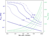 |
Fig. 1 Equilibrium partial pressures of CO2 (dark blue) and NH3 (green) in Titan’s primordial atmosphere as a function of the total NH3 dissolved in the ocean. Each set of green and blue curves, distinguished by different line styles, represents a specified initial CO2 atmospheric pressure prior to chemical equilibrium between the ocean and atmosphere. The initial theoretical PCO2 values of 1, 5, 10, 20, and 30 bar correspond to CO2 bulk masses of 7.8 × 10¹⁹ kg, 3.79 × 10²⁰ kg, 7.38 × 10²⁰ kg, 1.37 × 10²⁰ kg, and 1.92 × 1030 kg, and a dissolved CO2 mole fraction of 1.36 × 10⁻³, 6.78 × 10⁻³, 1.36 × 10⁻², 2.71 × 10⁻², and 4.07 × 10⁻², respectively. |
3 Results
We investigated the composition of Titan’s primordial hydrosphere during two distinct phases: the open-ocean phase, when the ocean directly interacted with the atmosphere, and the closed-ocean phase, when an icy crust formed, isolating the ocean from atmospheric exchange.
3.1 Combined evolution of Titan’s ocean and atmosphere compositions during the open-ocean phase
The composition and evolution of Titan’s primordial hydrosphere were examined based on a specific bulk composition, with particular emphasis on the role of NH3, whose abundance ranges from 1.5 to 15 wt% in the ocean (Tobie et al. 2012). The dissolution of ammonia and carbon dioxide in the global ocean can significantly influence atmospheric composition and thickness through the chemical balance between NH3 and CO2 speciation products. In particular, the ratio of dissolved CO2 to NH3 is a key factor in determining whether a CO2-rich atmosphere can be sustained (Marounina et al. 2018; Amsler Moulanier et al. 2025).
Figure 1 presents the equilibrium partial pressures of CO2 and NH3 in Titan’s primordial atmosphere at 273.15 K, as a function of the total NH3 fraction in the ocean and the theoretical initial CO2 partial pressure. The results indicate that when the NH3 concentration exceeds 2%, even an initially high atmospheric CO2 abundance (>10 bar) cannot be sustained above Titan’s primordial ocean. This finding challenges the hypothesis that Titan once hosted a thick CH4- and CO2-rich primordial atmosphere (Lunine et al. 2009; Tobie et al. 2014) in direct contact with an NH3-rich ocean (Lunine & Stevenson 1987; Tobie et al. 2012). It also raises questions about the feasibility of surface clathrate formation during the open-ocean phase, since this process requires the total atmospheric pressure to exceed the clathrate dissociation pressure. As shown by Marounina et al. (2018), we suggest that, in the temperature range considered, a thick CO2-rich primordial atmosphere in equilibrium with a NH3-rich ocean would not have been sustainable.
The composition of Titan’s primordial atmosphere, and its relative tendency to favor CO2 or NH3, is inferred from its primordial bulk composition. Here, Titan’s volatile inventory is assumed to have originated from volatile-rich icy planetesimals with a comet-like composition, with the volatile fraction in the ice phase analogous to that measured in comet 67P/Churyumov-Gerasimenko (67P/C-G) (Rubin et al. 2019). Given Titan’s bulk density, the total mass of ice in its composition is assumed to be ~50% (Lunine et al. 2009; Tobie et al. 2012). In this study, we assumed that about 30% of Titan’s mass contributed to the melting of ice that formed the primordial atmosphere and ocean (Lunine et al. 2009), corresponding to a melted ice fraction of 60%. By computing the normalized volatile mass distribution in ice, we could estimate the total bulk mass of each volatile delivered to Titan’s hydrosphere (see Table 1). Based on this volatile inventory, Titan’s primordial ocean would be approximately 500 km deep. If the melted ice fraction were to reach 80% (Monteux et al. 2014), the partial pressures above the ocean would increase. Specifically, higher CO2 pressures could support the existence of liquid CO2. However, a higher surface pressure could promote clathrate formation at a temperature slightly higher than 282 K if 80% of the ice melts.
Using our model (Appendix A), we computed the thermodynamic equilibrium between the primordial atmosphere ocean and how volatiles are partitioned between the two phases. Assuming comet-like building blocks, a significant amount of CO2 is released from the ice (4.12 × 10²¹ kg). Our computations show that such a mass of CO2 introduced into the hydrosphere would lead to a considerable pressure at Titan’s surface. To model a physically accurate system, we capped the initial partial pressure of CO2 at its saturation pressure as computed with Antoine’s law. As mentioned previously, both CO2 and NH3 should be present within the primordial hydrosphere of Titan in significant proportion. Although NH3 has a higher solubility than CO2, Table 1 shows that at 273.15 K a thick CO2 atmosphere forms at the ocean surface, while most of NH3 is speciated and retained in the ocean as ions (![Mathematical equation: $\[\mathrm{NH}_{4}^{+}\]$](/articles/aa/full_html/2025/06/aa54398-25/aa54398-25-eq5.png) and NH2COO−) leading to a limited fraction of free NH3 present within the ocean. This conclusion particularly contrasts with the assumption of a primordial NH3-rich global ocean on Titan (Tobie et al. 2012). The formation of a CO2-rich atmosphere is, however, consistent with the findings of Ishimaru et al. (2011), which supports the idea that a CO2-rich oxidized primordial atmosphere could have allowed the formation of N2 from NH3 via impact shock chemistry.
and NH2COO−) leading to a limited fraction of free NH3 present within the ocean. This conclusion particularly contrasts with the assumption of a primordial NH3-rich global ocean on Titan (Tobie et al. 2012). The formation of a CO2-rich atmosphere is, however, consistent with the findings of Ishimaru et al. (2011), which supports the idea that a CO2-rich oxidized primordial atmosphere could have allowed the formation of N2 from NH3 via impact shock chemistry.
Figure 2 illustrates the effect of temperature on the composition of Titan’s primordial atmosphere and ocean at equilibrium. As the temperature decreases from 300 K to 273.15 K, the atmosphere becomes less dense and the fraction of dissolved volatiles increases. The magnitude of this change varies with the gas under consideration. For example, in this temperature range, the partial pressure of Xe decreases by 24%, while the abundance of Ar in the atmosphere is only slightly affected (8%). In contrast, the evolution of the CO2 and NH3 abundances in the atmosphere and ocean follows a distinct trajectory, determined by their chemical equilibrium in the ocean.
Bulk masses, partial pressures (Pi), and mole fractions (xi) of the main volatile species at equilibrium between the primordial atmosphere and ocean at 273.15 K.
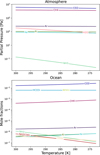 |
Fig. 2 Evolution of the composition of Titan’s primordial atmosphere and ocean at equilibrium, as a function of surface temperature. |
3.2 Effect of clathrate formation on the composition of the primordial atmosphere during Titan’s closed-ocean phase
We focused on two stages of Titan’s evolution, corresponding to a surface temperature of 280 K and 273.15 K. At those temperatures, the equilibrium total surface pressure falls within the mixed clathrate stability region, with boundaries calculated using Eq. (1). This boundary is reached when the surface temperature drops to 282 K, allowing clathrates to form on top of the ocean, still uncovered by the ice crust. In our model, we assumed that the clathration process halts when the surface pressure falls below the dissociation pressure of mixed clathrates. At 280 K and 273.15 K, we calculated the clathrate composition and assessed its impact on the distribution of volatiles in the atmosphere. Figure 3 illustrates the distribution of partial pressures as a function of mixed clathrate crust thickness. The detection limit of the Huygens GCMS instrument for volatile abundances (indicated in dashed black on the figure), set at 10−8 (corresponding to a maximum partial pressure of approximately 1.5 × 10⁻³ Pa; Niemann et al. 2005), serves as the threshold for determining when a gas can be considered depleted from the atmosphere. At 280 K, close to the mixed clathrate stability limit, a 1.23 km thick crust can form until the surface pressure becomes too low to allow clathrate stability. At such a low thickness, the noble gases are not trapped in significant proportions. Titan’s surface must cool to reduce the dissociation pressure of the clathrates, thereby trapping more gases. At 273 K, Xe is almost completely removed from the atmosphere, becoming sufficiently rare to be undetectable by the Huygens GCMS – when the clathrate crust reaches a thickness of 3.3 km. In contrast, trapping all of the Kr in the atmosphere requires a thicker crust, as this noble gas is less efficiently trapped than Xe. Hence, Kr is almost completely trapped in clathrates with a crust thickness of 10.31 km.
However, Ar is much less efficiently trapped in clathrates compared to other noble gases and cannot be sufficiently captured before reaching the maximum crust thickness of 11 km at 273 K. For Ar to be completely removed from the primordial atmosphere, Titan’s surface would need to cool further. Based on the total surface pressure before crust formation and the Ar abundance shown in Table 1, our calculations suggest that complete trapping of Ar in clathrates – whether mixed or pure – likely did not occur during Titan’s early history.
Additionally, a shift in the composition of the mixed clathrates occurs as the crust thickens and time progresses. This transition is highlighted in Fig. 3 by the dashed red line, marking a change in the dominant gas forming the clathrate. To the left of this line, CH4 is the primary gas captured in the clathrate, despite being less abundant than CO2 in the atmosphere, due to thermodynamic conditions favoring its trapping. To the right of the red line, however, CH4 becomes too scarce in the atmosphere, and CO2 takes over as the driving force for clathrate formation. This shift in the dominant clathrate-forming gas significantly alters the overall composition of the mixed clathrates, as shown in Fig. 3, and consequently affects the composition of the crust over time. As shown in Fig. 4, this change in composition leads to a variation in clathrate density. As the crust thickens and clathrates shift from a CH4-rich to a CO2-rich composition, the density of the clathrates increases, surpassing a value of 1. As a result, while CH4-rich clathrates would float on the ocean, the more recent CO2-rich upper layers become denser than the older, lower layers, exceeding the density of liquid water when ρ > 1. This density gradient could eventually lead to structural remodeling of the clathrate crust over time.
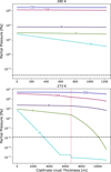 |
Fig. 3 Evolution of atmospheric abundances as a function of clathrate crust thickness at 280 and 273.15 K. The dashed red line indicates the threshold at which the clathrate composition changes from CH4-rich to CO2-rich. The dashed black line represents the detection limit of Huygens’ GCMS. |
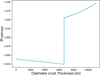 |
Fig. 4 Density of clathrates as a function of crust thickness, assuming formation at 273 K. The step for both temperatures highlights the transition from CH4-rich to denser CO2-rich clathrates. |
3.3 Formation of a crustal CH4-rich reservoir
Titan’s atmosphere features a ~5% CH4 fraction measured at its surface by Huygens (Niemann et al. 2005). Since CH4 is destroyed by UV photochemistry on 10–100 Myr timescales (Yung et al. 1984; Wilson & Atreya 2004), this suggests replenishment from an internal reservoir containing at least ~2.8 × 10¹⁷ kg of CH4 to maintain this level over 4.5 billion years (Niemann et al. 2005).
Assuming a comet-like primordial bulk composition, we estimated that Titan’s primordial atmosphere at 300 K contained at least 9.4 × 10¹⁹ kg of CH4, providing a sufficient initial reservoir. Once clathrates form, our calculations show that at 273.15 K, with a 11 km-thick crust, about 7.76 × 10¹⁹ kg of CH4 would be retained. Thus, a clathrate crust just below a dozen kilometers thick could store enough CH4 to serve as a long-term reservoir to maintain Titan’s atmospheric composition. Based on the current mass of CH4 in Titan’s atmosphere, we estimate that the reservoir could replenish the atmosphere for at least 2.8 Gyr.
4 Discussion and conclusions
This study explores clathrate formation during Titan’s primordial phase as a key factor in its present-day noble gas depletion. If Titan’s volatiles originated from comet-like building blocks, a CO2- and CH4-rich atmosphere would have formed over a liquid water ocean depleted of free NH3. In this ocean, the CO2–NH3 equilibrium would have converted most NH3 into ![Mathematical equation: $\[\mathrm{NH}_{4}^{+}\]$](/articles/aa/full_html/2025/06/aa54398-25/aa54398-25-eq6.png) . Notably, if the NH3 concentration in the ocean did not exceeded a few percent (which is compatible with existing constrains on comets and Enceladus data), the primordial atmosphere should be dominated by CO2. As temperatures fell to 282 K and below, clathrates could have formed a crust on the surface of Titan’s ocean, incorporating Xe and Kr into a CH4- and CO2-rich structure and thereby accounting for their depletion in the atmosphere. In particular, if this clathrate crust reached a thickness of about 10 km at 273.15 K during Titan’s early evolution, it could have efficiently sequestered Xe and Kr from the atmosphere. However, this process could not fully remove Ar, differing from Mousis et al. (2011) due to variations in atmospheric composition. We propose that Titan accreted from planetesimals that partially devolatilized in Saturn’s sub-nebula (Mousis et al. 2009b), which would explain the absence of primordial Ar. This clathrate formation may have also retained CH4, contributing to its long-term atmospheric replenishment.
. Notably, if the NH3 concentration in the ocean did not exceeded a few percent (which is compatible with existing constrains on comets and Enceladus data), the primordial atmosphere should be dominated by CO2. As temperatures fell to 282 K and below, clathrates could have formed a crust on the surface of Titan’s ocean, incorporating Xe and Kr into a CH4- and CO2-rich structure and thereby accounting for their depletion in the atmosphere. In particular, if this clathrate crust reached a thickness of about 10 km at 273.15 K during Titan’s early evolution, it could have efficiently sequestered Xe and Kr from the atmosphere. However, this process could not fully remove Ar, differing from Mousis et al. (2011) due to variations in atmospheric composition. We propose that Titan accreted from planetesimals that partially devolatilized in Saturn’s sub-nebula (Mousis et al. 2009b), which would explain the absence of primordial Ar. This clathrate formation may have also retained CH4, contributing to its long-term atmospheric replenishment.
We emphasize that the modeling carried out in this study does not account for the clathrate formation kinetics, which is a critical aspect in this process. Specifically, our results highlighting the capture of Kr and Xe during Titan’s primordial phase at 273.15 K are valid only if the clathrate crust formation occurred while the surface temperature remained at 273.15 K. Indeed, a comparison between the cooling rate of Titan and the growth rate of the clathrate crust would be necessary but remains challenging given the current state of the art. Moreover, as the crust thickens, the transport of fresh water to the surface and/or the transport of gas through the clathrate crust should be limited, affecting the capture of noble gases from the atmosphere.
The case of argon can be considered a critical aspect in our study. Argon mainly exists as 40Ar in Titan’s atmosphere (Niemann et al. 2010). This isotope likely originated in the rocky mantle as 40K, which subsequently decayed into 40Ar and was transported into the ocean (Tobie et al. 2012). Its presence in the atmosphere suggests outgassing from the icy crust, where it may have interacted with clathrates (Tobie et al. 2014). However, given the low trapping efficiency of Ar in clathrate hydrates (Thomas et al. 2007, 2008), we propose that, in competition with other dissolved species such as CH4 and CO2, 40Ar most likely escaped from the crust without being incorporated into clathrates.
Finally, the bulk composition scenario and the results presented in this study raise the following questions:
If a thick, primordial CO2-rich atmosphere formed from comet-like building blocks shortly after Titan’s accretion, what processes could account for the low present-day abundance of CO2? Beyond clathrate sequestration, several plausible mechanisms include surface condensation as Titan cooled (Lunine et al. 2009), early atmospheric escape (Kuramoto & Matsui 1994), photolysis, and loss through impact-driven chemistry (Ishimaru et al. 2011);
If N2 formation from NH3 via shock chemistry is possible in a CO2-rich atmosphere (Ishimaru et al. 2011), what mechanism could sustain NH3 in the atmosphere, considering its expected retention in the ocean under such conditions? Possible processes include continuous outgassing from the interior, photochemical recycling, or impact-driven volatilization (Sekine et al. 2011);
If primordial clathrates containing CH4, Ar, Kr, and Xe act as a reservoir for CH4, how can CH4 be released without simultaneously reintroducing noble gases – specifically, 3.74 × 10¹⁶ kg of Xe and 5.65 × 10¹⁶ kg of Kr-into the atmosphere? One possibility is that Xe and Kr remain sequestered in residual surface clathrates during CH4 release, or are reenclathrated shortly thereafter. This implies the existence of an additional mechanism that prevents their effective outgassing (Thomas et al. 2008; Mousis et al. 2011). The existence of such a mechanism is supported by the strong thermodynamic preference of Xe and Kr for clathrate formation compared to other gases (Sloan & Koh 2008).
Acknowledgements
O.M. and A.B. acknowledge support from CNES. The project leading to this publication has received funding from the Excellence Initiative of Aix-Marseille Université – A*Midex, a French “Investissements d’Avenir programme” AMX-21-IET-018. This research holds as part of the project FACOM (ANR-22-CE49-0005-01 ACT) and has benefited from a funding provided by l’Agence Nationale de la Recherche (ANR) under the Generic Call for Proposals 2022.
Appendix A Description of the atmosphere-ocean equilibrium
The model presented in this section follows the approach outlined in Marounina et al. (2018), which models the H2O–CO2–NH3 system based on previous works (Göppert & Maurer 1988; Pazuki et al. 2006; Darde et al. 2010). Our ocean equilibrium model, developed in Amsler Moulanier et al. (2025) and in this study, shares several similarities with Marounina et al. (2018), particularly the use of the Peng-Robinson-Gasem equation of state (EOS) for fugacity coefficients of gases and the extended UNIQUAC model for activity coefficients of dissolved species. However, several key differences distinguish our model:
The standard-state fugacity of dissolved species is approximated using Henry’s law constant, with an added Poynting correction factor.
The van der Waals one-fluid mixing rule is incorporated in the Peng-Robinson EOS to account for gas interactions.
Constants such as Henry’s constants, Ki dissociation constants, and Tc, Pc, and ωc values are sourced from different references.
The activity coefficient for CH4 is computed.
Clathrate formation at the surface of the primordial ocean is included. A key novelty of our model is simulating the impact of clathrate formation on the evolution of the primordial atmosphere. Additionally, the composition of clathrates is computed through fractional occupancies of guest molecules, using a statistical thermodynamic model.
The components of our model are outlined below.
A.1 Liquid-vapor equilibrium
We computed the liquid-vapor equilibrium for each species starting from the equality between the vapor and liquid phases’ fugacities, ![Mathematical equation: $\[f_{i}^{V}\]$](/articles/aa/full_html/2025/06/aa54398-25/aa54398-25-eq7.png) and
and ![Mathematical equation: $\[f_{i}^{L}\]$](/articles/aa/full_html/2025/06/aa54398-25/aa54398-25-eq8.png) , respectively:
, respectively:
![Mathematical equation: $\[f_i^V\left(T, P, y_i\right)=f_i^L\left(T, P, x_i\right).\]$](/articles/aa/full_html/2025/06/aa54398-25/aa54398-25-eq9.png) (A.1)
(A.1)
Here, the fugacity of the species i in the vapor phase, ![Mathematical equation: $\[f_{i}^{V}\]$](/articles/aa/full_html/2025/06/aa54398-25/aa54398-25-eq10.png) , is a function of temperature T, pressure P, and mole fraction yi in the vapor phase. Likewise, the fugacity of the species i in the liquid phase,
, is a function of temperature T, pressure P, and mole fraction yi in the vapor phase. Likewise, the fugacity of the species i in the liquid phase, ![Mathematical equation: $\[f_{i}^{L}\]$](/articles/aa/full_html/2025/06/aa54398-25/aa54398-25-eq11.png) , is a function of T, P, and mole fraction xi in the liquid phase.
, is a function of T, P, and mole fraction xi in the liquid phase.
To account for the nonideal behavior in the gas phase and the nonideal interactions between the dissolved species in the liquid phase, we introduced respectively the fugacity coefficient (ϕ) and the activity coefficient (γ). Hence, the fugacity of each phase for an individual species i can be written as
![Mathematical equation: $\[\begin{aligned}& f_i^V=\phi_i y_i P,\\& f_i^L=\gamma_i x_i f_i^0.\end{aligned}\]$](/articles/aa/full_html/2025/06/aa54398-25/aa54398-25-eq12.png) (A.2)
(A.2)
In the vapor phase, the fugacity ![Mathematical equation: $\[f_{i}^{V}\]$](/articles/aa/full_html/2025/06/aa54398-25/aa54398-25-eq13.png) of the specie i is a function of the fugacity coefficient ϕi, the mole fraction yi, and the total pressure P in Pascal. In the liquid phase, the fugacity
of the specie i is a function of the fugacity coefficient ϕi, the mole fraction yi, and the total pressure P in Pascal. In the liquid phase, the fugacity ![Mathematical equation: $\[f_{i}^{L}\]$](/articles/aa/full_html/2025/06/aa54398-25/aa54398-25-eq14.png) is a function of the activity coefficient γi, the mole fraction xi, and the standard-state fugacity
is a function of the activity coefficient γi, the mole fraction xi, and the standard-state fugacity ![Mathematical equation: $\[f_{i}^{0}\]$](/articles/aa/full_html/2025/06/aa54398-25/aa54398-25-eq15.png) .
.
Then, we were able to compute the partitioning of volatiles between the atmosphere and the ocean, taking the nonideal behavior of both phases into account, by substituting these expressions into Eq. (A.1). The standard-state fugacity ![Mathematical equation: $\[(f_{i}^{0})\]$](/articles/aa/full_html/2025/06/aa54398-25/aa54398-25-eq16.png) of H2O is set to the saturation pressure of water,
of H2O is set to the saturation pressure of water, ![Mathematical equation: $\[P_{{H}_{2}{O}}^{s}(T)\]$](/articles/aa/full_html/2025/06/aa54398-25/aa54398-25-eq17.png) , which is calculated using Antoine’s equation (Stull 1947):
, which is calculated using Antoine’s equation (Stull 1947):
![Mathematical equation: $\[\log _{10}\left(P_{H_2 O}^s\right)=A-\frac{B}{T+C},\]$](/articles/aa/full_html/2025/06/aa54398-25/aa54398-25-eq18.png) (A.3)
with A = 4.6543, B = 1435.264, C = −64.848, T in K and P in bar.
(A.3)
with A = 4.6543, B = 1435.264, C = −64.848, T in K and P in bar.
Equation (A.2) can then be rewritten as
![Mathematical equation: $\[\begin{aligned}& \phi_{{H}_2 {O}} ~P ~y_{{H}_2 {O}}=\gamma_{{H}_2 {O}} ~x_{{H}_2 {O}} ~P_{{H}_2 {O}}^s(T) \\& \phi_i P y_i=\gamma_i ~x_i ~H_{{H}_2 {O}, i}(T) ~\exp~ \left(\frac{v_{i, {H}_2 {O}}^{\infty}\left(P-P_{{H}_2 {O}}^s\right)}{R T}\right),\end{aligned}\]$](/articles/aa/full_html/2025/06/aa54398-25/aa54398-25-eq19.png) (A.4)
where the standard-state fugacity
(A.4)
where the standard-state fugacity ![Mathematical equation: $\[f_{i}^{0}\]$](/articles/aa/full_html/2025/06/aa54398-25/aa54398-25-eq20.png) of dissolved species i is approximated as the Henry’s law constant, corrected by a Poynting factor (Kawazuishi & Prausnitz 1987; Darde et al. 2010). The Henry’s law constants and their temperature dependences are reported in Table A.1 and were taken from Kawazuishi & Prausnitz (1987) for CO2 and NH3, and from Warneck & Williams (2012) for the other species.
of dissolved species i is approximated as the Henry’s law constant, corrected by a Poynting factor (Kawazuishi & Prausnitz 1987; Darde et al. 2010). The Henry’s law constants and their temperature dependences are reported in Table A.1 and were taken from Kawazuishi & Prausnitz (1987) for CO2 and NH3, and from Warneck & Williams (2012) for the other species.
The molar volume of the species i at infinite dilution, ![Mathematical equation: $\[v_{i, H_{2} O}^{\infty}\]$](/articles/aa/full_html/2025/06/aa54398-25/aa54398-25-eq21.png) , is extrapolated from Rumpf & Maurer (1993a,b) and Garcia (2001) for CO2 and NH3. For the other species,
, is extrapolated from Rumpf & Maurer (1993a,b) and Garcia (2001) for CO2 and NH3. For the other species, ![Mathematical equation: $\[v_{i, H_{2} O}^{\infty}\]$](/articles/aa/full_html/2025/06/aa54398-25/aa54398-25-eq22.png) is set to 0. R is the ideal gas constant.
is set to 0. R is the ideal gas constant.
We computed the fugacity coefficient (ϕi) for each species using the Peng-Robinson EOS (Peng & Robinson 1976) and the van der Waals one-fluid mixing rule. The molar volume of the mixture v was derived from the Peng-Robinson EOS:
![Mathematical equation: $\[P=\frac{R T}{v-b}-\frac{a \alpha}{v^2+2 v b-b^2},\]$](/articles/aa/full_html/2025/06/aa54398-25/aa54398-25-eq23.png) (A.5)
where
(A.5)
where
![Mathematical equation: $\[\begin{aligned}& a=\frac{0.457235 R^2 T_c^2}{P_c}, \\& b=\frac{0.077796 R T_c}{P_c}, \\& \alpha=\left(1+\kappa\left(1-\sqrt{\frac{T}{T_c}}\right)\right)^2,\end{aligned}\]$](/articles/aa/full_html/2025/06/aa54398-25/aa54398-25-eq24.png) (A.6)
and κ = 0.37464 + 1.54226ω − 0.2699ω2.
(A.6)
and κ = 0.37464 + 1.54226ω − 0.2699ω2.
Here, Tc is the critical temperature, Pc is the critical pressure, and ω is the acentric factor of each volatile. Their values are shown in Table A.2.
The mixture parameters Amix and Bmix required for the Peng-Robinson EOS and the van der Waals one-fluid mixing rule were computed using the following equations:
![Mathematical equation: $\[\begin{aligned}A_i= & ~a_i \times \alpha_i, \\A_{i j}= & ~\left(1-k_{i j}\right) \sqrt{A_i A_j}, \\A_{\text {mix }}= & \sum_i^N \sum_j^N y_i y_j A_{i j}, \\\text { and } B_{{mix }}= & \sum_i^N y_i b_i,\end{aligned}\]$](/articles/aa/full_html/2025/06/aa54398-25/aa54398-25-eq25.png) (A.7)
(A.7)
Henry’s constants’ interpolation formulas of gases in water.
where N is the total number of species. αi, ai and bi are computed for each species i using Eq. A.6. In order to better capture the nonideal behavior of the volatile mixtures in the atmosphere and ocean, binary interaction coefficients kij are used to further account for the nonideal interactions between the volatile species, following the approach described in Gasem et al. (2001). If they are not available in the literature, they are set to 0. These binary interaction coefficients are determined empirically and taken from the literature (Dhima et al. (1999) for H2O-CO2, and Vrabec et al. (2009) for the other couples). After calculating the molar volume v from the Peng-Robinson EOS (Eq. A.5), the fugacity coefficient ϕi of a species i can be derived from Eq. A.5:
![Mathematical equation: $\[\begin{aligned}\ln \left(\phi_i(T, v, y)\right) & =\frac{b_i}{B_{{mix }}}(Z-1)-\ln \left(\frac{P}{R T}\left(v-B_{{mix }}\right)\right)+ \\& \frac{A_{{mix }}}{2 \sqrt{2} R T B_{{mix }}} \ln \left(\frac{v+B_{{mix }} 2.414}{v-B_{{mix }} 0.414}\right)\end{aligned}\]$](/articles/aa/full_html/2025/06/aa54398-25/aa54398-25-eq26.png) (A.8)
with,
(A.8)
with, ![Mathematical equation: $\[Z=\frac{Pv}{RT}\]$](/articles/aa/full_html/2025/06/aa54398-25/aa54398-25-eq27.png) .
.
The activity coefficients of H2O, CO2 and NH3 are computed with the extended UNIQUAC model (Thomsen & Rasmussen 1999). The activity coefficient of CH4 is taken from Kvamme (2021). For the other neutral species, we set γi = 1.
Tc, Pc, and ω values used in the model (Reid et al. 1987).
A.2 Chemical equilibrium
The liquid-vapor equilibrium is coupled with the chemical equilibrium taking place within the aqueous H2O-CO2-NH3 system:
![Mathematical equation: $\[{H}_2 {O} \rightleftharpoons {H}^{+}+{OH}^{-},\]$](/articles/aa/full_html/2025/06/aa54398-25/aa54398-25-eq28.png) (A.9)
(A.9)
![Mathematical equation: $\[{CO}_2+{H}_2 {O} \rightleftharpoons {HCO}_3^{-}+{H}^{+},\]$](/articles/aa/full_html/2025/06/aa54398-25/aa54398-25-eq29.png) (A.10)
(A.10)
![Mathematical equation: $\[{NH}_3+{H}_2 {O} \rightleftharpoons {NH}_4^{+}+{OH}^{-},\]$](/articles/aa/full_html/2025/06/aa54398-25/aa54398-25-eq30.png) (A.11)
(A.11)
![Mathematical equation: $\[{HCO}_3^{-} \rightleftharpoons {CO}_3^{2-}+{H}^{+},\]$](/articles/aa/full_html/2025/06/aa54398-25/aa54398-25-eq31.png) (A.12)
(A.12)
![Mathematical equation: $\[{HCO}_3^{-}+{NH}_3 \rightleftharpoons {NH}_2 {COO}^{-}+{H}_2 {O}.\]$](/articles/aa/full_html/2025/06/aa54398-25/aa54398-25-eq32.png) (A.13)
(A.13)
The equations describing the chemical equilibrium within the H2O-CO2-NH3 system are derived from the dissociation reactions of these species:
![Mathematical equation: $\[K_{{H}_2 {O}}=\frac{m_{{OH}^{-}} m_{{H}^{+}}}{x_{{H}_2 {O}}} \frac{\gamma_{{OH}^{-}} \gamma_{{H}^{+}}}{\gamma_{{H}_2 {O}}},\]$](/articles/aa/full_html/2025/06/aa54398-25/aa54398-25-eq33.png) (A.14)
(A.14)
![Mathematical equation: $\[K_{{CO}_2}=\frac{m_{{HCO}_3^{-}} m_{{H}^{+}}}{x_{{H}_2 {O}} m_{{CO}_2}} \frac{\gamma_{{HCO}_3^{-}} \gamma_{{H}^{+}}}{\gamma_{{H}_2 {O}} \gamma_{{CO}_2}},\]$](/articles/aa/full_html/2025/06/aa54398-25/aa54398-25-eq34.png) (A.15)
(A.15)
![Mathematical equation: $\[K_{{NH}_3}=\frac{m_{{NH}_4^{+}} m_{{OH}^{-}}}{x_{{H}_2 {O}} m_{{NH}_3}} \frac{\gamma_{{NH}_4^{+}} \gamma_{{OH}^{-}}}{\gamma_{{H}_2 {O}} \gamma_{{NH}_3}},\]$](/articles/aa/full_html/2025/06/aa54398-25/aa54398-25-eq35.png) (A.16)
(A.16)
![Mathematical equation: $\[K_{{HCO}_3^{-}}=\frac{m_{{CO}_3^{2-}} m_{{H}^{+}}}{m_{{HCO}_3^{-}}} \frac{\gamma_{{CO}_3^{2-}} \gamma_{{H}^{+}}}{\gamma_{{HCO}_3^{-}}},\]$](/articles/aa/full_html/2025/06/aa54398-25/aa54398-25-eq36.png) (A.17)
(A.17)
![Mathematical equation: $\[K_{{NH}_2 {COO}^{-}}=\frac{m_{{NH}_2 {COO}^{-}} x_{{H}_2 {O}}}{m_{{NH}_3} m_{{HCO}_3^{-}}} \frac{\gamma_{{NH}_2 {COO}^{-}} \gamma_{{H}_2 {O}}}{\gamma_{{NH}_3} \gamma_{{HCO}_3^{-}}},\]$](/articles/aa/full_html/2025/06/aa54398-25/aa54398-25-eq37.png) (A.18)
where Ki(T) is the dissociation constant of each reaction taken from Kawazuishi & Prausnitz (1987), mi (in mol/kg) is the molality of the aqueous species, xH2O the mole fraction of water, and γi the activity coefficient of the species i.
(A.18)
where Ki(T) is the dissociation constant of each reaction taken from Kawazuishi & Prausnitz (1987), mi (in mol/kg) is the molality of the aqueous species, xH2O the mole fraction of water, and γi the activity coefficient of the species i.
To compute the activity coefficients involved in the chemical equilibrium equations, we used the extended UNIQUAC model, first introduced in Thomsen & Rasmussen (1999) and the parameters from Darde et al. (2010). This model calculates the activity coefficient using combinatorial, residual, and electrostatic terms, with the electrostatic terms based on the extended Debye-Hückel law. It is well established for studying this specific chemical equilibrium (Thomsen & Rasmussen 1999; Thomsen 2005; Darde et al. 2010). Finally, we could compute the whole set of variables using the mass and charge balance equations derived as follows:
![Mathematical equation: $\[m_{{CO}_{2 { tot }}}=m_{{CO}_2}+m_{{HCO}_3^{-}}+m_{{CO}_3^{2-}}+m_{{NH}_2 {COO}^{-}},\]$](/articles/aa/full_html/2025/06/aa54398-25/aa54398-25-eq38.png) (A.19)
(A.19)
![Mathematical equation: $\[m_{{NH}_{3 { tot }}}=m_{{NH}_3}+m_{{NH}_4^{+}}+m_{{NH}_2 {COO}^{-}},\]$](/articles/aa/full_html/2025/06/aa54398-25/aa54398-25-eq39.png) (A.20)
(A.20)
![Mathematical equation: $\[m_{{H}^{+}}+m_{{NH}_4^{+}}=m_{{OH}^{-}}+m_{{HCO}_3^{-}}+2 m_{{CO}_3^{2-}}+m_{{NH}_2 {COO}^{-}},\]$](/articles/aa/full_html/2025/06/aa54398-25/aa54398-25-eq40.png) (A.21)
where mCO2tot and mNH3tot are the total molalities of CO2 and NH3 incorporated into the liquid phase.
(A.21)
where mCO2tot and mNH3tot are the total molalities of CO2 and NH3 incorporated into the liquid phase.
Appendix B Clathrate formation model
B.1 The statistical thermodynamic model
The method described in this section, detailed in Mousis et al. (2013), uses classical statistical mechanics to describe the macroscopic thermodynamic properties of clathrates to the molecular structure and interaction energies. It is based on the original model of van der Waals & Platteeuw (1959), which assumes that trapping of guest molecules into cages corresponds to the three-dimensional generalization of ideal localized adsorption. It is based on four hypotheses:
The contribution of the host molecules to the free energy is independent of the clathrate occupancy. This implies that the guest species do not distort the cages.
The cages are singly occupied, and guest molecules rotate freely within the cage.
Guest molecules do not interact with each other.
Classical statistics is valid, meaning that quantum effects are negligible.
Hence, the fractional occupancy of a guest molecule i for a given type of cage q (small or large) in a clathrate structure can be written as
![Mathematical equation: $\[y_{i, q}=\frac{C_{i, q} f_{h y d r o, i}}{1+\sum_J C_{J, q} f_{h y d r o, J}},\]$](/articles/aa/full_html/2025/06/aa54398-25/aa54398-25-eq41.png) (B.1)
where the sum in the denominator includes all the species present in the gas. Ci,q is the Langmuir constant of the species i in the cage of type q, fhydro,i is the fugacity of the guest species i computed at the total gas pressure (see Appendix B.2).
(B.1)
where the sum in the denominator includes all the species present in the gas. Ci,q is the Langmuir constant of the species i in the cage of type q, fhydro,i is the fugacity of the guest species i computed at the total gas pressure (see Appendix B.2).
The Langmuir constant Ci,q depends on the strength of the interaction between each guest species and each type of cage. It can be calculated by integrating the molecular potential energy within the cavity as
![Mathematical equation: $\[C_{i, q}=\frac{4 \pi}{k_B T} \int_0^{R_c} exp \left(-\frac{w_{i, q}(r)}{k_B T}\right) r^2 d r,\]$](/articles/aa/full_html/2025/06/aa54398-25/aa54398-25-eq42.png) (B.2)
where Rc represents the radius of the cavity assumed to be spherical, kB its the Boltzmann constant, and wi,q(r) is the spherically averaged potential (here Kiahara or Lennard-Jones potential) representing the interactions between the guest molecules i and the water molecules forming the surrounding cage q. This potential wi,q(r) can be written for a spherical guest molecule as (McKoy & Sinanoğlu 1963)
(B.2)
where Rc represents the radius of the cavity assumed to be spherical, kB its the Boltzmann constant, and wi,q(r) is the spherically averaged potential (here Kiahara or Lennard-Jones potential) representing the interactions between the guest molecules i and the water molecules forming the surrounding cage q. This potential wi,q(r) can be written for a spherical guest molecule as (McKoy & Sinanoğlu 1963)
![Mathematical equation: $\[w(r)=2 z \epsilon\left[\frac{\sigma^{12}}{R_c^{11} r}\left(\delta^{10}(r)+\frac{a}{R_c} \delta^{11}(r)\right)-\frac{\sigma^6}{R_c^5 r}\left(\delta^4(r)+\frac{a}{R_c} \delta^5(r)\right)\right],\]$](/articles/aa/full_html/2025/06/aa54398-25/aa54398-25-eq43.png) (B.3)
with the mathematical function δN(r) in the form
(B.3)
with the mathematical function δN(r) in the form
![Mathematical equation: $\[\delta^N(r)=\frac{1}{N}\left[\left(1-\frac{r}{R_c}-\frac{a}{R_c}\right)^{-N}-\left(1+\frac{r}{R_c}-\frac{a}{R_c}\right)^{-N}\right].\]$](/articles/aa/full_html/2025/06/aa54398-25/aa54398-25-eq44.png) (B.4)
(B.4)
In Eq. B.3, z is the coordination number of the cell. Parameters z and Rc depend on the cage type q (small or large) and on the clathrate structure (I or II). Their values are given in Table B.1. The intermolecular parameters a, σ and ϵ describing the guest molecule i-water (i-W) interactions in the form of a Kihara or Lennard-Jones potential are listed in Table B.2.
Finally, the mole fraction ![Mathematical equation: $\[x_{i}^{clath}\]$](/articles/aa/full_html/2025/06/aa54398-25/aa54398-25-eq45.png) of a guest molecule i in a clathrate of a given structure (I or II) can be computed as
of a guest molecule i in a clathrate of a given structure (I or II) can be computed as
![Mathematical equation: $\[x_i^{{clath }}=\frac{b_s y_{i, s}+b_l y_{i, l}}{b_s \sum_J y_{J, s}+b_l \sum_J y_{J, l}},\]$](/articles/aa/full_html/2025/06/aa54398-25/aa54398-25-eq46.png) (B.5)
where bs and bl are the number of small and large cages per unit cell, respectively, for the clathrate structure we considered. The mole fractions of the enclathrated species is normalized to 1.
(B.5)
where bs and bl are the number of small and large cages per unit cell, respectively, for the clathrate structure we considered. The mole fractions of the enclathrated species is normalized to 1.
Parameters for the clathrate cavities.
B.2 Calculation of the fugacities
To determine fhydro,i, we first calculated the specific volume (v) of the considered mixture via the Redlich-Kwong EOS (Redlich & Kwong 1949):
![Mathematical equation: $\[P=\frac{R T}{v-b}-\frac{a}{\sqrt{T} v(v+b)}\]$](/articles/aa/full_html/2025/06/aa54398-25/aa54398-25-eq47.png) (B.6)
with
(B.6)
with
![Mathematical equation: $\[a=0.4278 \frac{R^2 T_c^{2.5}}{P_c}, \qquad\qquad b=0.08664 \frac{R T_c}{P_c}\]$](/articles/aa/full_html/2025/06/aa54398-25/aa54398-25-eq48.png) (B.7)
where R is the perfect gas constant, T the ambient temperature, Tc and Pc the critical temperature and pressure of the substance i Tab. A.2. In this case, a and b account for a pure substance. For mixtures, we took the average properties of the mixture into account by using the mixing rules
(B.7)
where R is the perfect gas constant, T the ambient temperature, Tc and Pc the critical temperature and pressure of the substance i Tab. A.2. In this case, a and b account for a pure substance. For mixtures, we took the average properties of the mixture into account by using the mixing rules
![Mathematical equation: $\[\begin{array}{ll}a_m=\sum_i \sum_j y_i y_j a_{i j} &\quad\quad \text { with } a_{i j}=\sqrt{a_i a_j}, \\b_m=\sum_i y_i b_i, &\end{array}\]$](/articles/aa/full_html/2025/06/aa54398-25/aa54398-25-eq49.png) (B.8)
where yi the molar fraction of the gas in the atmosphere, normalized for the enclathrated species to 1. Then, we defined the mixture pressure Pm dissolved in water, which corresponds to the sum of the individual dissolved pressure Pi. This pressure is different than the partial pressure of the gas in the atmosphere. It is expressed as a function of Henry’s law coefficient as
(B.8)
where yi the molar fraction of the gas in the atmosphere, normalized for the enclathrated species to 1. Then, we defined the mixture pressure Pm dissolved in water, which corresponds to the sum of the individual dissolved pressure Pi. This pressure is different than the partial pressure of the gas in the atmosphere. It is expressed as a function of Henry’s law coefficient as
![Mathematical equation: $\[P_i=H_{{hydro }, i} \times y_i,\]$](/articles/aa/full_html/2025/06/aa54398-25/aa54398-25-eq50.png) (B.9)
where Hhydro,i is the Henry’s law constant calculated for specie i at the surface (hydrostatic) pressure Ptot and temperature T. It is calculated as
(B.9)
where Hhydro,i is the Henry’s law constant calculated for specie i at the surface (hydrostatic) pressure Ptot and temperature T. It is calculated as
![Mathematical equation: $\[\ln \left(\frac{H_{{hydro }, i}}{H_{1 a t m, i}}\right)=\frac{\bar{V}_i}{R T}\left(P_{t o t}-1.013 \times 10^5\right),\]$](/articles/aa/full_html/2025/06/aa54398-25/aa54398-25-eq51.png) (B.10)
where H1atm,i is the Henry’s constant of specie i calculated at 1 atmosphere and 0°C and
(B.10)
where H1atm,i is the Henry’s constant of specie i calculated at 1 atmosphere and 0°C and ![Mathematical equation: $\[\bar{V}_{i}\]$](/articles/aa/full_html/2025/06/aa54398-25/aa54398-25-eq52.png) is the partial molar volume of specie i. The fugacity of the mixture at 1 atm pressure (f1atm,m) can be computed as (Redlich & Kwong 1949)
is the partial molar volume of specie i. The fugacity of the mixture at 1 atm pressure (f1atm,m) can be computed as (Redlich & Kwong 1949)
![Mathematical equation: $\[\begin{aligned}& \ln f_{1 a t m, m}=\frac{b_m}{v_m-b_m}+\ln \frac{R T}{v_m-b_m}- \\& \frac{a_m}{R T^{3 / 2}}\left(\frac{1}{v_m+b_m}+\frac{1}{b_m} \ln \frac{\left(v_m+b_m\right)}{v_m}\right)\end{aligned}.\]$](/articles/aa/full_html/2025/06/aa54398-25/aa54398-25-eq53.png) (B.11)
(B.11)
Parameters for the Kihara and Lennard-Jones potentials.
The fugacity of the mixture calculated at the surface pressure fhydro,m is related to f1atm,m via (Miller 1974)
![Mathematical equation: $\[\ln \frac{f_{{hydro }, m}}{f_{1 a t m, m}}=-n {\ln} a_w-\frac{P_{t o t}-1.013 \times 10^5}{R T}\left(v V_{{H}_2 {O}}-V_{c, m}\right),\]$](/articles/aa/full_html/2025/06/aa54398-25/aa54398-25-eq54.png) (B.12)
where aw is the activity of water relative to pure liquid water (~1 here), n is the moles of water per mole of species i in the clathrate (n ~ 6), VH2O is the molar volume of liquid water (1.8 × 10⁻⁵ m3) and Vc,m is the volume of clathrate that contains 1 mol of substance m. Finally, the fugacity coefficient ϕ of the mixture can be computed from
(B.12)
where aw is the activity of water relative to pure liquid water (~1 here), n is the moles of water per mole of species i in the clathrate (n ~ 6), VH2O is the molar volume of liquid water (1.8 × 10⁻⁵ m3) and Vc,m is the volume of clathrate that contains 1 mol of substance m. Finally, the fugacity coefficient ϕ of the mixture can be computed from
![Mathematical equation: $\[f_{{hydro }, i}=\phi \times P_i.\]$](/articles/aa/full_html/2025/06/aa54398-25/aa54398-25-eq55.png) (B.13)
(B.13)
The values of ![Mathematical equation: $\[T_{c}, P_{c}, \bar{V}_{i}, H_{1 a t m, i}\]$](/articles/aa/full_html/2025/06/aa54398-25/aa54398-25-eq56.png) and f1atm,i used for each species i are taken from Mousis et al. (2013) Table 1.
and f1atm,i used for each species i are taken from Mousis et al. (2013) Table 1.
B.3 Calculation of clathrate density
From the calculation of the fractional occupancies (yi,q) in both small and larges cages, it is possible to derive the clathrate density based upon a unit crystal (Sloan & Koh 2008):
![Mathematical equation: $\[\rho=\frac{N_w M_{H_2 O}+\sum_{q=1}^C \sum_{i=1}^N y_{i, q} b_q M_i}{N_{{Ava}} V_{{cell}}},\]$](/articles/aa/full_html/2025/06/aa54398-25/aa54398-25-eq57.png) (B.14)
where NW is the number of water molecules per unit cell, NAna is Avogadro’s number (6.023 × 10²³), Mi the molecular weight of molecule i, yi,q is the fractional occupancy of molecule i in type q cavity (small or large), bq is the number of type q cavities per water molecules in unit cell, Vcell is the volume of an unit cell, N is the number of cavity type per unit cell (in this case 2) and C the number of component trapped in hydrate phase. Nw, bq and Vcell values are given in Table B.1 for each structure (I and II).
(B.14)
where NW is the number of water molecules per unit cell, NAna is Avogadro’s number (6.023 × 10²³), Mi the molecular weight of molecule i, yi,q is the fractional occupancy of molecule i in type q cavity (small or large), bq is the number of type q cavities per water molecules in unit cell, Vcell is the volume of an unit cell, N is the number of cavity type per unit cell (in this case 2) and C the number of component trapped in hydrate phase. Nw, bq and Vcell values are given in Table B.1 for each structure (I and II).
References
- Alibert, Y., & Mousis, O. 2007, A&A, 465, 1051 [NASA ADS] [CrossRef] [EDP Sciences] [Google Scholar]
- Amsler Moulanier, A., Mousis, O., Bouquet, A., & Glein, C. R. 2025, Planet. Sci. J., 6, 1 [Google Scholar]
- Atreya, S. K., Donahue, T. M., & Kuhn, W. R. 1978, Science, 201, 611 [Google Scholar]
- Darde, V., van Well, W. J. M., Stenby, E. H., & Thomsen, K. 2010, Ind. Eng. Chem. Res., 49, 12663 [Google Scholar]
- Dhima, A., de Hemptinne, J.-C., & Jose, J. 1999, Ind. Eng. Chem. Res., 38, 3144 [Google Scholar]
- Englezos, P., Kalogerakis, N., Dholabhai, P., & Bishnoi, P. 1987, Chem. Eng. Sci., 42, 2659 [Google Scholar]
- Garcia, J. E. 2001, Density of aqueous solutions of CO2, Tech. Rep. LBNL-49023, 790022 [CrossRef] [Google Scholar]
- Gasem, K., Gao, W., Pan, Z., & Robinson, R. 2001, Fluid Phase Equilibria, 181, 113 [Google Scholar]
- Glein, C. R., Desch, S. J., & Shock, E. L. 2009, Icarus, 204, 637 [Google Scholar]
- Grasset, O., & Sotin, C. 1996, Icarus, 123, 101 [Google Scholar]
- Göppert, U., & Maurer, G. 1988, Fluid Phase Equilibria, 41, 153 [Google Scholar]
- Ishimaru, R., Sekine, Y., Matsui, T., & Mousis, O. 2011, ApJ, 741, L10 [Google Scholar]
- Jones, T. D., & Lewis, J. S. 1987, Icarus, 72, 381 [Google Scholar]
- Kawazuishi, K., & Prausnitz, J. M. 1987, Ind. Eng. Chem. Res., 26, 1482 [Google Scholar]
- Kuramoto, K., & Matsui, T. 1994, J. Geophys. Res.: Planets, 99, 21183 [NASA ADS] [CrossRef] [Google Scholar]
- Kvamme, B. 2021, Fluids, 6, 345 [Google Scholar]
- Lipenkov, V. Y., & Istomin, V. A. 2001, Mater. Glyatsiol. Issled., 91, 129 [Google Scholar]
- Lunine, J. I., & Stevenson, D. J. 1987, Icarus, 70, 61 [Google Scholar]
- Lunine, J. I., & Nolan, M. C. 1992, Icarus, 100, 221 [NASA ADS] [CrossRef] [Google Scholar]
- Lunine, J. I., Atreya, S. K., & Pollack, J. B. 1989, Present State and Chemical Evolution of the Atmospheres of Titan, Triton, and Pluto, 605 [Google Scholar]
- Lunine, J., Choukroun, M., Stevenson, D., & Tobie, G. 2009, in Titan from Cassini-Huygens, eds. R. H. Brown, J.-P. Lebreton, & J. H. Waite (Dordrecht: Springer Netherlands), 35 [CrossRef] [Google Scholar]
- Marounina, N., Grasset, O., Tobie, G., & Carpy, S. 2018, Icarus, 310, 127 [Google Scholar]
- McKoy, V., & Sinanoğlu, O. 1963, J. Chem. Phys., 38, 2946 [Google Scholar]
- McKay, C. P., Scattergood, T. W., Pollack, J. B., Borucki, W. J., & Ghyseghem, H. T. V. 1988, Nature, 332, 520 [NASA ADS] [CrossRef] [Google Scholar]
- Miller, S. L. 1974, in Natural Gases in Marine Sediments, ed. I. R. Kaplan (Boston, MA: Springer US), 151 [CrossRef] [Google Scholar]
- Monteux, J., Tobie, G., Choblet, G., & Le Feuvre, M. 2014, Icarus, 237, 377 [Google Scholar]
- Mousis, O., Lunine, J. I., Pasek, M., et al. 2009a, Icarus, 204, 749 [Google Scholar]
- Mousis, O., Lunine, J. I., Thomas, C., et al. 2009b, ApJ, 691, 1780 [Google Scholar]
- Mousis, O., Marboeuf, U., Lunine, J. I., et al. 2009c, ApJ, 696, 1348 [NASA ADS] [CrossRef] [Google Scholar]
- Mousis, O., Lunine, J. I., Picaud, S., et al. 2011, ApJ, 740, L9 [Google Scholar]
- Mousis, O., Lakhlifi, A., Picaud, S., Pasek, M., & Chassefière, E. 2013, Astrobiology, 13, 380 [Google Scholar]
- Niemann, H. B., Atreya, S. K., Bauer, S. J., et al. 2005, Nature, 438, 779 [Google Scholar]
- Niemann, H. B., Atreya, S. K., Demick, J. E., et al. 2010, J. Geophys. Res.: Planets, 115, 2010JE003659 [Google Scholar]
- Osegovic, J. P., & Max, M. D. 2005, J. Geophys. Res.: Planets, 110, 2005JE002435 [Google Scholar]
- Parrish, W. R., & Prausnitz, J. M. 1972, Ind. Eng. Chem. Process Des. Dev., 11, 26 [CrossRef] [Google Scholar]
- Pazuki, G., Pahlevanzadeh, H., & Ahooei, A. M. 2006, Fluid Phase Equilibria, 242, 57 [Google Scholar]
- Peng, D.-Y., & Robinson, D. B. 1976, Ind. Eng. Chem. Fundam., 15, 59 [CrossRef] [Google Scholar]
- Redlich, O., & Kwong, J. N. S. 1949, Chem. Rev., 44, 233 [Google Scholar]
- Reid, R., Prausnitz, J. M., & Poling, B. 1987, The Properties of Gases & Liquids 4th edn. (New York: McGraw-Hill) [Google Scholar]
- Reynard, B., & Sotin, C. 2023, Earth Planet. Sci. Lett., 612, 118172 [Google Scholar]
- Rubin, M., Altwegg, K., Balsiger, H., et al. 2019, MNRAS, 489, 594 [Google Scholar]
- Rumpf, B., & Maurer, G. 1993a, Berichte Bunsengesell. Physikal. Chem., 97, 85 [Google Scholar]
- Rumpf, B., & Maurer, G. 1993b, Ind. Eng. Chem. Res., 32, 1780 [Google Scholar]
- Ruppel, C. D., & Waite, W. F. 2020, J. Geophys. Res.: Solid Earth, 125, e2018JB016459 [Google Scholar]
- Sekine, Y., Genda, H., Sugita, S., Kadono, T., & Matsui, T. 2011, Nat. Geosci., 4, 359 [NASA ADS] [CrossRef] [Google Scholar]
- Sloan, E., & Koh, C. A. 2008, Clathrate Hydrates of Natural Gases, 3rd edn. (CRC Press) [Google Scholar]
- Stull, D. R. 1947, Ind. Eng. Chem., 39, 517 [CrossRef] [Google Scholar]
- Thomsen, K. 2005, Pure Appl. Chem., 77, 531 [Google Scholar]
- Thomas, C., Mousis, O., Ballenegger, V., & Picaud, S. 2007, A&A, 474, L17 [NASA ADS] [CrossRef] [EDP Sciences] [Google Scholar]
- Thomas, C., Picaud, S., Mousis, O., & Ballenegger, V. 2008, Planet. Space Sci., 56, 1607 [Google Scholar]
- Thomsen, K., & Rasmussen, P. 1999, Chem. Eng. Sci., 54, 1787 [Google Scholar]
- Tobie, G., Gautier, D., & Hersant, F. 2012, ApJ, 752, 125 [Google Scholar]
- Tobie, G., Lunine, J. I., Monteux, J., Mousis, O., & Nimmo, F. 2014, in Titan: Interior, Surface, Atmosphere, and Space Environment. I. Müller-Wodarg, C. A. Griffith, E. Lellouch, & T. E. Cravens, Cambridge Planetary Science (Cambridge: Cambridge University Press), 29 [Google Scholar]
- Uchida, T., Moriwaki, M., Takeya, S., et al. 2004, AIChE J., 50, 518 [Google Scholar]
- Vrabec, J., Huang, Y.-l., & Hasse, H. 2009, Fluid Phase Equilibria, 279, 120 [Google Scholar]
- van der Waals, J. H., & Platteeuw, J. C. 1959, in Advances in Chemical Physics, (Wiley), 1 [Google Scholar]
- Waite, J. H., Lewis, W. S., Magee, B. A., et al. 2009, Nature, 460, 487 [NASA ADS] [CrossRef] [Google Scholar]
- Warneck, P., & Williams, J. 2012, The Atmospheric Chemist’s Companion: Numerical Data for Use in the Atmospheric Sciences (Dordrecht: Springer Netherlands) [CrossRef] [Google Scholar]
- Wilson, E. H., & Atreya, S. K. 2004, J. Geophys. Res.: Planets, 109, 2003JE002181 [Google Scholar]
- Yung, Y. L., Allen, M., & Pinto, J. P. 1984, ApJS, 55, 465 [NASA ADS] [CrossRef] [Google Scholar]
All Tables
Bulk masses, partial pressures (Pi), and mole fractions (xi) of the main volatile species at equilibrium between the primordial atmosphere and ocean at 273.15 K.
All Figures
|
Fig. 1 Equilibrium partial pressures of CO2 (dark blue) and NH3 (green) in Titan’s primordial atmosphere as a function of the total NH3 dissolved in the ocean. Each set of green and blue curves, distinguished by different line styles, represents a specified initial CO2 atmospheric pressure prior to chemical equilibrium between the ocean and atmosphere. The initial theoretical PCO2 values of 1, 5, 10, 20, and 30 bar correspond to CO2 bulk masses of 7.8 × 10¹⁹ kg, 3.79 × 10²⁰ kg, 7.38 × 10²⁰ kg, 1.37 × 10²⁰ kg, and 1.92 × 1030 kg, and a dissolved CO2 mole fraction of 1.36 × 10⁻³, 6.78 × 10⁻³, 1.36 × 10⁻², 2.71 × 10⁻², and 4.07 × 10⁻², respectively. |
| In the text | |
|
Fig. 2 Evolution of the composition of Titan’s primordial atmosphere and ocean at equilibrium, as a function of surface temperature. |
| In the text | |
|
Fig. 3 Evolution of atmospheric abundances as a function of clathrate crust thickness at 280 and 273.15 K. The dashed red line indicates the threshold at which the clathrate composition changes from CH4-rich to CO2-rich. The dashed black line represents the detection limit of Huygens’ GCMS. |
| In the text | |
|
Fig. 4 Density of clathrates as a function of crust thickness, assuming formation at 273 K. The step for both temperatures highlights the transition from CH4-rich to denser CO2-rich clathrates. |
| In the text | |
Current usage metrics show cumulative count of Article Views (full-text article views including HTML views, PDF and ePub downloads, according to the available data) and Abstracts Views on Vision4Press platform.
Data correspond to usage on the plateform after 2015. The current usage metrics is available 48-96 hours after online publication and is updated daily on week days.
Initial download of the metrics may take a while.