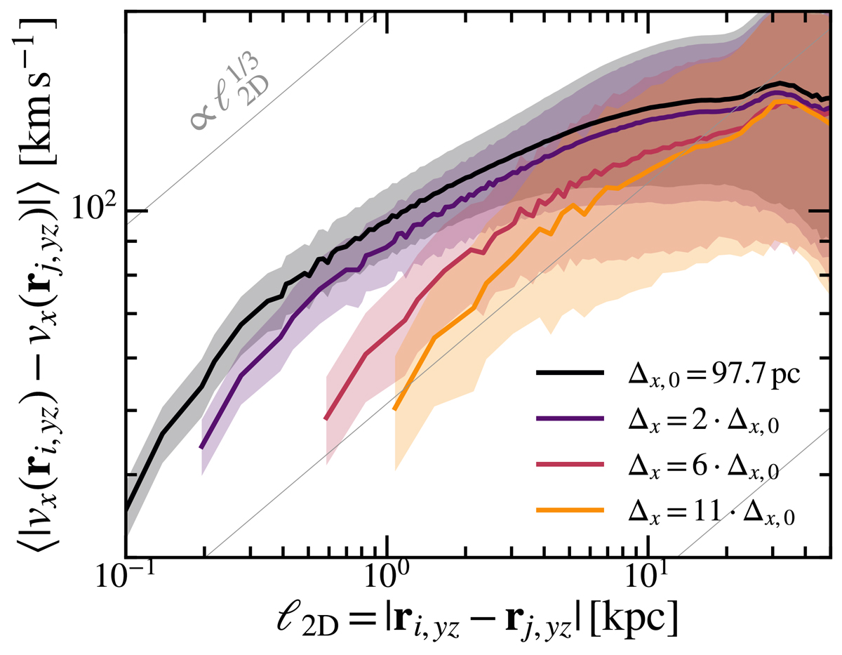
Velocity structure functions obtained from projected maps taking various spatial resolutions for the cold gas located at a projected radius of r ≤ 25 kpc. The projection method for all curves is equivalent to the third curve in Fig. 8 (i.e., labeled as ℓ_yz + w(Hα)). Consequently, the VSFs presented here are shallower than their three-dimensional counterparts (labeled as ℓ_3D in Fig. 8) due to projection and emission weighting. The darkest curve corresponds to the maximum spatial resolution Δ_x, 0 of our simulation. All brighter curves are obtained from coarse-grained maps with pixel size Δ_x. The colored areas represent the standard deviation resulting from time variation across all snapshots.