Galaxy infall models for arbitrary velocity directions

Jenny Wagner; David Benisty

doi:10.1051/0004-6361/202553892

Home

All issues

Volume 698 (May 2025)

A&A, 698 (2025) A211

Full HTML

Open Access

Issue		A&A Volume 698, May 2025


Article Number		A211
Number of page(s)		13
Section		Extragalactic astronomy
DOI		https://doi.org/10.1051/0004-6361/202553892
Published online		17 June 2025

A&A, 698, A211 (2025)

Galaxy infall models for arbitrary velocity directions

Jenny Wagner¹^,2^,3^⋆ and David Benisty⁴^⋆

¹ Helsinki Institute of Physics, P.O. Box 64 FI-00014 University of Helsinki, Finland
² Academia Sinica Institute of Astronomy and Astrophysics, 11F of AS/NTU Astronomy-Mathematics Building, No.1, Sec. 4, Roosevelt Rd, Taipei 106216, Taiwan, ROC
³ Bahamas Advanced Study Institute and Conferences, 4A Ocean Heights, Hill View Circle, Stella Maris, Long Island, The Bahamas
⁴ Leibniz-Institut für Astrophysik Potsdam (AIP), An der Sternwarte 16, 14482 Potsdam, Germany

^⋆ Corresponding authors: wagner@asiaa.sinica.edu.tw; benidav@aip.de

Received: 24 January 2025
Accepted: 15 May 2025

Abstract

For most galaxies in the cosmos, our knowledge of their motion is limited to line-of-sight velocities from redshift observations. To determine the radial velocity between two galaxies, the “minor” and “major infall models” were established by Igor Karachentsev and colleagues. Regardless of the background cosmology, our derivations reveal that these infall models approximate the total radial velocity between two galaxies by two different projections employing different information about the system. For galaxies that have small angular separations, θ, all infall models agree that the radial velocity is the difference of their line-of-sight components. Applying these models to around 500 halos of the Illustris-3 simulation, we find the perpendicular and tangential velocity parts to be non-negligible for more than 90% of over 5000 infalling subhalos investigated. Thus, even for θ < 10 deg, the infall-model velocities deviate from the true radial velocity. Only for 30% did we find the true one lay between the minor and major infall velocity. However, the infall models yield robust upper and lower limits to the true radial velocity dispersion. Observed under θ < 10 deg, the velocity dispersion inferred from the sole difference of line-of-sight velocity components even coincides with the true one, justifying this approach for high-redshift groups and clusters. Based on these findings, we predict the radial velocity dispersion of the M81 group from the minor infall model (upper bound) to be σ_r, min = (180 ± 42) km/s, from the major infall model (lower bound) to be σ_r, maj = (142 ± 64) km/s and σ_r, Δv = (99 ± 36) km/s from the line-of-sight-velocity difference.

Key words: techniques: radial velocities / astrometry / galaxies: kinematics and dynamics / galaxies: statistics / galaxies: groups: individual: M81

© The Authors 2025

Open Access article, published by EDP Sciences, under the terms of the Creative Commons Attribution License (https://creativecommons.org/licenses/by/4.0), which permits unrestricted use, distribution, and reproduction in any medium, provided the original work is properly cited.

This article is published in open access under the Subscribe to Open model. Subscribe to A&A to support open access publication.

1. Introduction

Studying the relative motion between cosmic structures is complicated for observers like us who are located at a random external position. In the majority of cases, external observers only measure velocity components along their lines of sight to the cosmic objects. This is often done with highly precise spectroscopic redshift observations. Most objects, such as galaxies, do not have a directly observable peculiar motion on the observer’s celestial sky. For instance, the peculiar motion for our neighbour-galaxy, M31, was inferred from peculiar-motion measurements of its stars and modelling of its satellite dwarf galaxy motions (Sohn et al. 2012; van der Marel et al. 2012).

Depending on the distance to us, spectroscopic redshifts need to be partitioned into a contribution from a cosmological background model and the velocity on top of it. The latter task is difficult in our cosmic neighbourhood, where both contributions play an equally important role (see recent observations and estimates by Cosmicflows (Tully et al. 2023; Valade et al. 2024) or the Dark Energy Spectroscopic Instrument DESI Collaboration 2024; Said et al. 2025).

Reconstructing a self-consistent map of our cosmic neighbourhood of mass (density) distributions from galaxies, over groups to clusters and their motions, many models have been used. Two seminal works were Karachentsev & Kashibadze (2006) and Karachentsev & Nasonova (2010). They considered two limiting cases: the minor infall model assumes that galaxies are mainly moved by an expanding cosmological background, a linear Hubble flow, and are only subject to a small mutual gravitational attraction. The major infall model assumes that galaxies fall into the gravitational potential of a galaxy group or cluster instead of following the Hubble flow.

Both models neglect the velocity components perpendicular to the observer’s line of sight. They assume that the structure is spherically symmetric to calculate the radial infall velocity and that it is embedded in a linear Hubble flow. The authors then tried to select applications that obey these assumptions well and reduce the impact of the unknown tangential velocity component at the same time. Karachentsev & Kashibadze (2006) applied both models to the Local Group and the M81/M82 group, Karachentsev & Nasonova (2010) analysed the Virgo cluster. In Karachentsev & Kashibadze (2006) they probed the impact of the tangential velocity by a simulation. Following up, Kim et al. (2020) analysed the Hubble flow around Virgo and used minor and major infall velocities, after Sorce et al. (2016) only used the minor infall for a similar study. Even though there are only a few papers mentioning the names of these infall models, many works, such as Diaz et al. (2014), Peñarrubia et al. (2014), use the minor infall model to estimate the radial velocity component of binaries or galaxy groups.

To overcome these restrictions and to generalise the models for a deeper analytical understanding, we describe a general binary motion without assuming spherical symmetry or specifying the embedding cosmology. Staying on this general, kinematics-only level, it remains an open question as to whether the motions occur in a gravitationally bound or unbound volume. We also include the perpendicular velocity components in the models, detailed in Sect. 2. For the first time, we quantify their impact on the infall models and derive conditions under which the infall models yield lower or upper bounds to the true radial infall velocity. Analogously, we investigate the role of the tangential velocity. We also compare the two infall models with each other to derive the general conditions under which both models coincide. In Sect. 3, we then extend the formalism to galaxy groups or clusters and investigate the impact of the statistics on the accuracy of the models for larger structures. Section 4 applies the infall models to cosmic structures from a snapshot at redshift z = 0 simulated in the Illustris-3 dataset that is publicly available online¹ in order to investigate the limits of the models in a realistic setting. Subsequently, in Sect. 5, we revisit the M81 system to discuss the accuracy of the reconstruction that is possible given the findings in this work. Finally, Sect. 6 summarises our results and gives an outlook on the applicability of the generalised models.

2. Pairwise infall models

2.1. Definitions and notation

To simplify the calculations, we used three-dimensional vectors in bold-font, like r. Their amplitudes² are denoted with |r| and their directions in terms of unit vectors by $\hat{r}$ $\hat{\boldsymbol{r}}$ . Line-of-sight components are denoted by subscript l, while components perpendicular to the line of sight are denoted with ⊥ as subscript. By construction, their scalar product vanishes, r_l ⋅ r_⊥ = 0.

In this notation, let galaxy i at redshift z_i be at a (cosmological) distance r_i, moving at a total velocity v_i with respect to this observer. We partitioned v_i into a projection along the observer’s line of sight and one perpendicular to it as

$\begin{matrix} v_{l i} \equiv (v_{i} \cdot {\hat{r}}_{i}) {\hat{r}}_{i} = | v_{l i} | {\hat{r}}_{i}, v_{⊥ i} \equiv (v_{i} \cdot {\hat{r}}_{⊥ i}) {\hat{r}}_{⊥ i} = | v_{⊥ i} | {\hat{r}}_{⊥ i} . \end{matrix}$ $\begin{aligned} \boldsymbol{v}_{\mathrm{l} i} \equiv \left(\boldsymbol{v}_i \cdot \hat{\boldsymbol{r}}_i \right) \, \hat{\boldsymbol{r}}_i = \left| \boldsymbol{v}_{\mathrm{l} i} \right| \, \hat{\boldsymbol{r}}_i \;, \quad \boldsymbol{v}_{\perp i} \equiv \left(\boldsymbol{v}_i \cdot \hat{\boldsymbol{r}}_{\perp i} \right) \, \hat{\boldsymbol{r}}_{\perp i} = \left| \boldsymbol{v}_{\perp i} \right| \, \hat{\boldsymbol{r}}_{\perp i}. \end{aligned}$ (1)

Considering arbitrary motions of two galaxies i = 1, 2 with distances from the observer r₁ and r₂ and total velocities v₁ and v₂, respectively, Fig. 1 shows all distances, and velocity components. To split every vector in its amplitude and direction, we used |r_i| ≡ ∥r_i∥₂, i = 1, 2 and read off Fig. 1 that

$\begin{matrix} | r_{21} | & \equiv (| | r_{1} {| |}_{2}^{2} + | | r_{2} {| |}_{2}^{2} - 2 | | r_{1} {| |}_{2} | | r_{2} {| |}_{2} cos θ)^{1 / 2}, \end{matrix}$ $\begin{aligned} \left| \boldsymbol{r}_{21} \right|&\equiv \Big ( ||\boldsymbol{r}_1||_{2}^2 + ||\boldsymbol{r}_2||_{2}^2 - 2||\boldsymbol{r}_{1}||_2 ||\boldsymbol{r}_{2}||_2 \cos \theta \Big )^{1/2},\end{aligned}$ (2)

$\begin{matrix} {\hat{r}}_{21} & = \frac{r_{2} - r_{1}}{| r_{21} |} = \frac{| r_{2} | {\hat{r}}_{2} - | r_{1} | {\hat{r}}_{1}}{| r_{21} |} \equiv {\bar{r}}_{2} {\hat{r}}_{2} - {\bar{r}}_{1} {\hat{r}}_{1}, \end{matrix}$ $\begin{aligned} \hat{\boldsymbol{r}}_{21}&= \frac{\boldsymbol{r}_{2} - \boldsymbol{r}_{1}}{\left| \boldsymbol{r}_{21}\right|} = \frac{\left| \boldsymbol{r}_2 \right| \hat{\boldsymbol{r}}_{2} - \left| \boldsymbol{r}_1 \right| \hat{\boldsymbol{r}}_{1}}{\left| \boldsymbol{r}_{21} \right|} \equiv \overline{r}_2 \hat{\boldsymbol{r}}_{2} - \overline{r}_1 \hat{\boldsymbol{r}}_{1},\end{aligned}$ (3)

$\begin{matrix} {\hat{r}}_{21} & = ({\bar{r}}_{2} cos θ - {\bar{r}}_{1}) {\hat{r}}_{1} - {\bar{r}}_{2} sin θ {\hat{r}}_{⊥ 1}, \end{matrix}$ $\begin{aligned} \hat{\boldsymbol{r}}_{21}&= \left( \overline{r}_2 \cos \theta - \overline{r}_1 \right) \hat{\boldsymbol{r}}_1 - \overline{r}_2 \sin \theta \,\hat{\boldsymbol{r}}_{\perp 1},\end{aligned}$ (4)

$\begin{matrix} = ({\bar{r}}_{2} - {\bar{r}}_{1} cos θ) {\hat{r}}_{2} - {\bar{r}}_{1} sin θ {\hat{r}}_{⊥ 2}, \end{matrix}$ $\begin{aligned}&= \left( \overline{r}_2 - \overline{r}_1 \cos \theta \right) \hat{\boldsymbol{r}}_2 - \overline{r}_1 \sin \theta \, \hat{\boldsymbol{r}}_{\perp 2},\end{aligned}$ (5)

$\begin{matrix} {\hat{r}}_{i} \cdot {\hat{r}}_{⊥ i} & = 0, i = 1, 2, \end{matrix}$ $\begin{aligned} \hat{\boldsymbol{r}}_i \cdot \hat{\boldsymbol{r}}_{\perp i}&= 0, \quad i = 1,2,\end{aligned}$ (6)

$\begin{matrix} {\hat{r}}_{1} \cdot {\hat{r}}_{2} & = {\hat{r}}_{⊥ 1} \cdot {\hat{r}}_{⊥ 2} = cos θ, \end{matrix}$ $\begin{aligned} \hat{\boldsymbol{r}}_1 \cdot \hat{\boldsymbol{r}}_2&= \hat{\boldsymbol{r}}_{\perp 1} \cdot \hat{\boldsymbol{r}}_{\perp 2} = \cos \theta ,\end{aligned}$ (7)

$\begin{matrix} {\hat{r}}_{1} \cdot {\hat{r}}_{⊥ 2} & = - {\hat{r}}_{2} \cdot {\hat{r}}_{⊥ 1} = sin θ . \end{matrix}$ $\begin{aligned} \hat{\boldsymbol{r}}_1 \cdot \hat{\boldsymbol{r}}_{\perp 2}&= - \hat{\boldsymbol{r}}_2 \cdot \hat{\boldsymbol{r}}_{\perp 1} = \sin \theta . \end{aligned}$ (8)

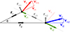Fig. 1.

Three-dimensional motion of two galaxies and definition of notations. The maximum information a distant observer can measure is the velocity components along the line of sight v_l1, v_l2 to a high precision via spectroscopy, highly precise angle between the galaxy positions on the sky, θ, and line-of-sight distances r₁, r₂ with a precision depending on the probe used (see Tully et al. 2023 for recent examples).

Eq. (8) can acquire a minus depending on the definition of r_⊥i. Here, it follows the definition of Fig. 1. The directions of r_i are chosen to be positive from the observer towards the galaxies. Hence the velocity amplitudes, |v_li|, can be positive or negative for i = 1, 2, depending on the relative orientation of the velocity with respect to the distance vector. There is no unique r_⊥i to r_i in three dimensions. Since only r_i and projections onto this vector yield observables, the non-uniqueness of r_⊥i implies that this component does not have a known direction in space. Only parts can be constrained by a projection onto the observer’s sky. Due to this freedom, r_⊥i are defined such that |v_⊥i| ≥ 0.

Similarly, we expressed the motion perpendicular to ${\hat{r}}_{21}$ $\hat{\boldsymbol{r}}_{21}$ . To calculate ${\hat{r}}_{⊥ 21}$ $\hat{\boldsymbol{r}}_{\perp 21}$ , we defined

$\begin{matrix} {\hat{n}}_{1} & = {\bar{r}}_{2} sin θ {\hat{r}}_{1} + ({\bar{r}}_{2} cos θ - {\bar{r}}_{1}) {\hat{r}}_{⊥ 1}, \end{matrix}$ $\begin{aligned} \hat{\boldsymbol{n}}_{1}&= \overline{r}_2 \sin \theta \, \hat{\boldsymbol{r}}_1 + \left(\overline{r}_2 \cos \theta - \overline{r}_1 \right) \hat{\boldsymbol{r}}_{\perp 1},\end{aligned}$ (9)

$\begin{matrix} {\hat{n}}_{2} & = {\bar{r}}_{1} sin θ {\hat{r}}_{2} + ({\bar{r}}_{2} - {\bar{r}}_{1} cos θ) {\hat{r}}_{⊥ 2}, \end{matrix}$ $\begin{aligned} \hat{\boldsymbol{n}}_{2}&= \overline{r}_1 \sin \theta \, \hat{\boldsymbol{r}}_2 + \left(\overline{r}_2 - \overline{r}_1 \cos \theta \right) \hat{\boldsymbol{r}}_{\perp 2}, \end{aligned}$ (10)

which obey $| {\hat{n}}_{i} | = 1$ $\left| \hat{\boldsymbol{n}}_i \right| = 1$ , ${\hat{r}}_{21} \cdot {\hat{n}}_{i} = 0$ $\hat{\boldsymbol{r}}_{21} \cdot \hat{\boldsymbol{n}}_{i} = 0$ , and ${\hat{n}}_{1} \cdot {\hat{n}}_{2} = 1$ $\hat{\boldsymbol{n}}_{1} \cdot \hat{\boldsymbol{n}}_{2} = 1$ , i = 1, 2. Since v_i = v_li + v_⊥i and there is no velocity component simultaneously perpendicular to ${\hat{r}}_{i}$ $\hat{\boldsymbol{r}}_i$ and ${\hat{r}}_{⊥ i}$ $\hat{\boldsymbol{r}}_{\perp i}$ , ${\hat{r}}_{⊥ 21} \equiv {\hat{n}}_{i}$ $\hat{\boldsymbol{r}}_{\perp 21} \equiv \hat{\boldsymbol{n}}_i$ , i = 1, 2.

Based on these relations, we derived

$\begin{matrix} {\hat{r}}_{1} \cdot {\hat{r}}_{21} & = {\bar{r}}_{2} cos θ - {\bar{r}}_{1}, \end{matrix}$ $\begin{aligned} \hat{\boldsymbol{r}}_1 \cdot \hat{\boldsymbol{r}}_{21}&= \overline{r}_2 \cos \theta - \overline{r}_1,\end{aligned}$ (11)

$\begin{matrix} {\hat{r}}_{2} \cdot {\hat{r}}_{21} & = {\bar{r}}_{2} - {\bar{r}}_{1} cos θ, \end{matrix}$ $\begin{aligned} \hat{\boldsymbol{r}}_2 \cdot \hat{\boldsymbol{r}}_{21}&= \overline{r}_2 - \overline{r}_1 \cos \theta ,\end{aligned}$ (12)

$\begin{matrix} {\hat{r}}_{⊥ 1} \cdot {\hat{r}}_{21} & = - {\bar{r}}_{2} sin θ, \end{matrix}$ $\begin{aligned} \hat{\boldsymbol{r}}_{\perp 1} \cdot \hat{\boldsymbol{r}}_{21}&= - \overline{r}_2 \sin \theta ,\end{aligned}$ (13)

$\begin{matrix} {\hat{r}}_{⊥ 2} \cdot {\hat{r}}_{21} & = - {\bar{r}}_{1} sin θ, \end{matrix}$ $\begin{aligned} \hat{\boldsymbol{r}}_{\perp 2} \cdot \hat{\boldsymbol{r}}_{21}&= - \overline{r}_1 \sin \theta ,\end{aligned}$ (14)

$\begin{matrix} {\hat{r}}_{1} \cdot {\hat{r}}_{⊥ 21} & = {\bar{r}}_{2} sin θ, \end{matrix}$ $\begin{aligned} \hat{\boldsymbol{r}}_1 \cdot \hat{\boldsymbol{r}}_{\perp 21}&= \overline{r}_2 \sin \theta ,\end{aligned}$ (15)

$\begin{matrix} {\hat{r}}_{2} \cdot {\hat{r}}_{⊥ 21} & = {\bar{r}}_{1} sin θ, \end{matrix}$ $\begin{aligned} \hat{\boldsymbol{r}}_2 \cdot \hat{\boldsymbol{r}}_{\perp 21}&= \overline{r}_1 \sin \theta ,\end{aligned}$ (16)

$\begin{matrix} {\hat{r}}_{⊥ 1} \cdot {\hat{r}}_{⊥ 21} & = ({\bar{r}}_{2} cos θ - {\bar{r}}_{1}), \end{matrix}$ $\begin{aligned} \hat{\boldsymbol{r}}_{\perp 1} \cdot \hat{\boldsymbol{r}}_{\perp 21}&= \left(\overline{r}_2 \cos \theta - \overline{r}_1 \right),\end{aligned}$ (17)

$\begin{matrix} {\hat{r}}_{⊥ 2} \cdot {\hat{r}}_{⊥ 21} & = ({\bar{r}}_{2} - {\bar{r}}_{1} cos θ) . \end{matrix}$ $\begin{aligned} \hat{\boldsymbol{r}}_{\perp 2} \cdot \hat{\boldsymbol{r}}_{\perp 21}&= \left(\overline{r}_2 - \overline{r}_1 \cos \theta \right). \end{aligned}$ (18)

2.2. General infall model

In the notation of Sect. 2.1, the relative velocity between the two galaxies reads

$\begin{matrix} v_{21} \equiv v_{2} - v_{1} & = v_{l 2} - v_{l 1} + v_{⊥ 2} - v_{⊥ 1} \end{matrix}$ $\begin{aligned} \boldsymbol{v}_{21} \equiv \boldsymbol{v}_2 - \boldsymbol{v}_1&= \boldsymbol{v}_{\mathrm{l} 2} - \boldsymbol{v}_{\mathrm{l} 1} + \boldsymbol{v}_{\perp 2} - \boldsymbol{v}_{\perp 1}\end{aligned}$ (19)

$\begin{matrix} = | v_{l 2} | {\hat{r}}_{2} - | v_{l 1} | {\hat{r}}_{1} + | v_{⊥ 2} | {\hat{r}}_{⊥ 2} - | v_{⊥ 1} | {\hat{r}}_{⊥ 1} . \end{matrix}$ $\begin{aligned}&= \left| \boldsymbol{v}_{\mathrm{l} 2} \right| \hat{\boldsymbol{r}}_{2} - \left| \boldsymbol{v}_{\mathrm{l} 1} \right| \hat{\boldsymbol{r}}_{1} + \left| \boldsymbol{v}_{\perp 2} \right| \hat{\boldsymbol{r}}_{\perp 2} - \left| \boldsymbol{v}_{\perp 1} \right| \hat{\boldsymbol{r}}_{\perp 1}. \end{aligned}$ (20)

To infer their radial infall velocity, we projected Eq. (20) onto their connection line. Using Eqs. (2)–(18), we obtained

$\begin{matrix} | v_{r} | & \equiv (v_{2} - v_{1}) \cdot {\hat{r}}_{21} = (v_{l 2} - v_{l 1}) \cdot {\hat{r}}_{21} + (v_{⊥ 2} - v_{⊥ 1}) \cdot {\hat{r}}_{21} \end{matrix}$ $\begin{aligned} \left| \boldsymbol{v}_{\mathrm{r} } \right|&\equiv \left( \boldsymbol{v}_2 - \boldsymbol{v}_1 \right) \cdot \hat{\boldsymbol{r}}_{21} = \left( \boldsymbol{v}_{\mathrm{l} 2} - \boldsymbol{v}_{\mathrm{l} 1} \right) \cdot \hat{\boldsymbol{r}}_{21} + \left( \boldsymbol{v}_{\perp 2} - \boldsymbol{v}_{\perp 1} \right) \cdot \hat{\boldsymbol{r}}_{21}\end{aligned}$ (21)

$\begin{matrix} = | v_{l 1} | {\bar{r}}_{1} + | v_{l 2} | {\bar{r}}_{2} - cos θ (| v_{l 1} | {\bar{r}}_{2} + | v_{l 2} | {\bar{r}}_{1}) \\ + sin θ (| v_{⊥ 1} | {\bar{r}}_{2} - | v_{⊥ 2} | {\bar{r}}_{1}) . \end{matrix}$ $\begin{aligned}&= \left| \boldsymbol{v}_{\mathrm{l} 1} \right| \bar{r}_1 + \left| \boldsymbol{v}_{\mathrm{l} 2} \right| \bar{r}_2 - \cos \theta \left( \left| \boldsymbol{v}_{\mathrm{l} 1} \right| \bar{r}_2 + \left| \boldsymbol{v}_{\mathrm{l} 2} \right| \bar{r}_1 \right)\\ &\quad \qquad \qquad \qquad + \sin \theta \left( \left| \boldsymbol{v}_{\perp 1} \right| \bar{r}_2 - \left| \boldsymbol{v}_{\perp 2} \right|\bar{r}_1 \right). \end{aligned}$ (22)

Thus, the radial velocity is expressed via the observable quantities θ, r₁, r₂, v_l1, and v_l2 and the unknown quantities v_⊥1 and v_⊥2. As a derived quantity, |v_r| can have negative, positive, or zero values. To linear order in θ, Eq. (22) reads

$\begin{matrix} | v_{r} | \approx | v_{l 2} | - | v_{l 1} | + θ (| v_{⊥ 1} | {\bar{r}}_{2} - | v_{⊥ 2} | {\bar{r}}_{1}), \end{matrix}$ $\begin{aligned} \left| \boldsymbol{v}_{\mathrm{r} } \right| \approx \left| \boldsymbol{v}_{\mathrm{l} 2} \right| - \left| \boldsymbol{v}_{\mathrm{l} 1} \right| + \theta \left( \left| \boldsymbol{v}_{\perp 1} \right|\overline{r}_2 - \left| \boldsymbol{v}_{\perp 2} \right|\overline{r}_1 \right), \end{aligned}$ (23)

such that |v_r| is the difference between the line-of-sight components plus a perturbation.

Similarly, projecting Eq. (19) onto ${\hat{r}}_{⊥ 21}$ $\hat{\boldsymbol{r}}_{\perp 21}$ , we obtained the velocity component perpendicular to the radial component,

$\begin{matrix} | v_{t} | & \equiv (v_{2} - v_{1}) \cdot {\hat{r}}_{⊥ 21} \end{matrix}$ $\begin{aligned} \left| \boldsymbol{v}_{\mathrm{t} } \right|&\equiv \left( \boldsymbol{v}_2 - \boldsymbol{v}_1 \right) \cdot \hat{\boldsymbol{r}}_{\perp 21}\end{aligned}$ (24)

$\begin{matrix} = (v_{l 2} - v_{l 1}) \cdot {\hat{r}}_{⊥ 21} + (v_{⊥ 2} - v_{⊥ 1}) \cdot {\hat{r}}_{⊥ 21} \end{matrix}$ $\begin{aligned}&= \left( \boldsymbol{v}_{\mathrm{l} 2} - \boldsymbol{v}_{\mathrm{l} 1} \right) \cdot \hat{\boldsymbol{r}}_{\perp 21} + \left( \boldsymbol{v}_{\perp 2} - \boldsymbol{v}_{\perp 1} \right) \cdot \hat{\boldsymbol{r}}_{\perp 21}\end{aligned}$ (25)

$\begin{matrix} = sin θ (| v_{l 2} | {\bar{r}}_{1} - | v_{l 1} | {\bar{r}}_{2}) \end{matrix}$ $\begin{aligned}&= \sin \theta \left( \left| \boldsymbol{v}_{\mathrm{l} 2} \right| \overline{r}_1 - \left| \boldsymbol{v}_{\mathrm{l} 1} \right| \overline{r}_2 \right)\end{aligned}$ (26)

$\begin{matrix} + | v_{⊥ 2} | {\bar{r}}_{2} + | v_{⊥ 1} | {\bar{r}}_{1} - cos θ (| v_{⊥ 1} | {\bar{r}}_{2} + | v_{⊥ 2} | {\bar{r}}_{1}) \\ \approx | v_{⊥ 2} | - | v_{⊥ 1} | + θ (| v_{l 2} | {\bar{r}}_{1} - | v_{l 1} | {\bar{r}}_{2}) . \end{matrix}$ $\begin{aligned}&\quad + \left| \boldsymbol{v}_{\perp 2} \right| \overline{r}_2 + \left| \boldsymbol{v}_{\perp 1} \right| \overline{r}_1 - \cos \theta \left(\left| \boldsymbol{v}_{\perp 1} \right| \overline{r}_2 + \left| \boldsymbol{v}_{\perp 2} \right| \overline{r}_1 \right) \nonumber \\&\approx \left| \boldsymbol{v}_{\perp 2} \right| - \left| \boldsymbol{v}_{\perp 1} \right| + \theta \left( \left| \boldsymbol{v}_{\mathrm{l} 2} \right| \overline{r}_1 - \left| \boldsymbol{v}_{\mathrm{l} 1} \right| \overline{r}_2 \right). \end{aligned}$ (27)

We denoted this component the tangential velocity. As a derived quantity, it can have any negative, positive, or zero value. To leading order, |v_t| is proportional to the difference of the perpendicular velocity components plus a perturbation.

We also expressed the velocity difference as a combination of radial and tangential components,

$\begin{matrix} v_{2} - v_{1} \equiv v_{r} + v_{t} = | v_{r} | {\hat{r}}_{21} + | v_{t} | {\hat{r}}_{⊥ 21} . \end{matrix}$ $\begin{aligned} \boldsymbol{v}_2 - \boldsymbol{v}_1 \equiv \boldsymbol{v}_{\mathrm{r} } + \boldsymbol{v}_{\mathrm{t} } = \left| \boldsymbol{v}_{\mathrm{r} }\right| \hat{\boldsymbol{r}}_{21} + \left| \boldsymbol{v}_{\mathrm{t} } \right| \hat{\boldsymbol{r}}_{\perp 21}. \end{aligned}$ (28)

Since v_t is not observable in general, we read off Eq. (26), under which conditions |v_t| = 0. For arbitrary θ, we obtained the general relation between the unknown and known quantities,

$\begin{matrix} | v_{⊥ 1} | + | v_{⊥ 2} | \frac{{\bar{r}}_{2} - {\bar{r}}_{1} cos θ}{{\bar{r}}_{1} - {\bar{r}}_{2} cos θ} = \frac{sin θ (| v_{l 2} | {\bar{r}}_{1} - | v_{l 1} | {\bar{r}}_{2})}{{\bar{r}}_{2} cos θ - {\bar{r}}_{1}} \cdot \end{matrix}$ $\begin{aligned} \left| \boldsymbol{v}_{\perp 1} \right| + \left| \boldsymbol{v}_{\perp 2} \right| \frac{\overline{r}_2- \overline{r}_1 \cos \theta }{\overline{r}_1 - \overline{r}_2 \cos \theta } = \frac{\sin \theta \left( \left| \boldsymbol{v}_{\mathrm{l} 2} \right| \overline{r}_1 - \left| \boldsymbol{v}_{\mathrm{l} 1} \right| \overline{r}_2 \right)}{\overline{r}_2 \cos \theta - \overline{r}_1}\cdot \end{aligned}$ (29)

Two special cases are

$\begin{matrix} θ = 0 & \land | v_{⊥ 1} | = | v_{⊥ 2} |, \end{matrix}$ $\begin{aligned} \theta = 0&\quad \wedge \quad \left| \boldsymbol{v}_{\perp 1} \right| = \left| \boldsymbol{v}_{\perp 2} \right|,\end{aligned}$ (30)

$\begin{matrix} | v_{⊥ 1} | = | v_{⊥ 2} | \frac{{\bar{r}}_{2} - {\bar{r}}_{1} cos θ}{{\bar{r}}_{2} cos θ - {\bar{r}}_{1}} & \land {\bar{r}}_{2} | v_{l 1} | = {\bar{r}}_{1} | v_{l 2} | . \end{matrix}$ $\begin{aligned} \left| \boldsymbol{v}_{\perp 1} \right| = \left| \boldsymbol{v}_{\perp 2} \right| \frac{\overline{r}_2 - \overline{r}_1 \cos \theta }{\overline{r}_2 \cos \theta - \overline{r}_1}&\quad \wedge \quad \overline{r}_2 \left| \boldsymbol{v}_{\mathrm{l} 1} \right| = \overline{r}_1 \left| \boldsymbol{v}_{\mathrm{l} 2} \right|. \end{aligned}$ (31)

Thus, the conditions for a purely radial infall are fine-tuned relative velocity components. The cases stated in prior work like Eq. (30) within the measurement precision thus greatly depend on additional assumptions, such as spherical symmetry, to achieve the fine-tuning. Only selecting galaxies almost aligned on the observer’s line of sight is not sufficient to achieve |v_t| = 0.

Assuming the perpendicular velocity components are unknown in Eq. (22), we found that the last term containing these components vanishes for θ ≠ 0 and |r_i| ≠ 0 if

$\begin{matrix} | v_{⊥ 1} | {\bar{r}}_{2} = | v_{⊥ 2} | {\bar{r}}_{1} \Leftrightarrow (\frac{| v_{⊥ 1} |}{| v_{⊥ 2} |} = \frac{| r_{1} |}{| r_{2} |}) \lor (v_{⊥ 1} = v_{⊥ 2} = 0) . \end{matrix}$ $\begin{aligned} \left| \boldsymbol{v}_{\perp 1} \right| \bar{r}_2 = \left| \boldsymbol{v}_{\perp 2} \right|\bar{r}_1 \; \Leftrightarrow \; \left( \frac{\left| \boldsymbol{v}_{\perp 1} \right|}{\left| \boldsymbol{v}_{\perp 2} \right|} = \frac{\left| \boldsymbol{r}_1 \right|}{\left| \boldsymbol{r}_2 \right|} \right) \; \vee \; \left( \boldsymbol{v}_{\perp 1} = \boldsymbol{v}_{\perp 2} = 0 \right). \end{aligned}$ (32)

These insights have an important impact on the minor and major infall models as discussed below.

2.3. Minor infall: Projection on the connection line

In this infall model, originally defined to describe the motion of two galaxies whose velocities are dominated by their surrounding Hubble flow, |v_li| ≫ |v_⊥i|, their relative radial velocity is

$\begin{matrix} | v_{r, \min} | & \equiv (v_{l 2} - v_{l 1}) \cdot {\hat{r}}_{21} \end{matrix}$ $\begin{aligned} \left| \boldsymbol{v}_{\mathrm{r} ,\mathrm{min} } \right|&\equiv \left( \boldsymbol{v}_{\mathrm{l} 2} - \boldsymbol{v}_{\mathrm{l} 1} \right) \cdot \hat{\boldsymbol{r}}_{21}\end{aligned}$ (33)

$\begin{matrix} = | v_{l 1} | {\bar{r}}_{1} + | v_{l 2} | {\bar{r}}_{2} - cos θ (| v_{l 1} | {\bar{r}}_{2} + | v_{l 2} | {\bar{r}}_{1}), \end{matrix}$ $\begin{aligned}&= \left| \boldsymbol{v}_{\mathrm{l} 1} \right| \overline{r}_1 + \left| \boldsymbol{v}_{\mathrm{l} 2} \right| \overline{r}_2 - \cos \theta \left( \left| \boldsymbol{v}_{\mathrm{l} 1} \right| \overline{r}_2 + \left| \boldsymbol{v}_{\mathrm{l} 2} \right| \overline{r}_1 \right), \end{aligned}$ (34)

which neglects the last term in Eq. (22). Fig. 2 visualises the situation. For θ ≠ 0 and r_i ≠ 0, we found that the minor infall model is a good approximation to the true radial velocity, if one of the two options in Eq. (32) holds. We also read off Eqs. (22) and (34) that, for 0 < θ < π, |v_r| is under-estimated by Eq. (34) if |v_⊥1|/|v_⊥2| > |r₁|/|r₂|. Vice versa, |v_r| is over-estimated by Eq. (34) if |v_⊥1|/|v_⊥2| < |r₁|/|r₂|.

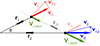Fig. 2.

Minor infall model: the line-of-sight velocity components of both galaxies are projected onto their connection line. The difference of these projections yields the relative radial velocity.

For v_i ≈ v_li, i = 1, 2, meaning v_⊥i ≈ 0, we found that Eq. (26) is reduced to the first term which consists of observable quantities up to the unknown direction of ${\hat{r}}_{⊥ 21}$ $\hat{\boldsymbol{r}}_{\perp 21}$ . So it is impossible to calculate v_t in general, which explains why the minor infall model does not make a statement about it. At best, we could exploit the fact that we observed θ with sin θ ∈ [−1;1] for v_i ≈ v_li to constrain |v_t| by

$\begin{matrix} - | | sin θ (| v_{l 2} | {\bar{r}}_{1} - | v_{l 1} | {\bar{r}}_{2}) {| |}_{2} \leq | v_{t} | \leq + | | sin θ (| v_{l 2} | {\bar{r}}_{1} - | v_{l 1} | {\bar{r}}_{2}) {| |}_{2} . \end{matrix}$ $\begin{aligned} - {||\sin \theta \left( \left| \boldsymbol{v}_{\mathrm{l} 2} \right| \overline{r}_1 - \left| \boldsymbol{v}_{\mathrm{l} 1} \right| \overline{r}_2 \right) ||_2} \le \left| \boldsymbol{v}_{\mathrm{t} } \right| \le + { ||\sin \theta \left( \left| \boldsymbol{v}_{\mathrm{l} 2} \right| \overline{r}_1 - \left| \boldsymbol{v}_{\mathrm{l} 1} \right| \overline{r}_2 \right) ||_2}. \end{aligned}$ (35)

2.4. Major infall: Projection on one line of sight

We first employed this infall model for two galaxies. Yet, we had already noted that the original approach replaced galaxy 2 by the centre of mass of a galaxy group and considered the infall of a galaxy onto the centre instead of a binary motion (see Sect. 3).

Shown in Fig. 3, the major infall model determines the radial velocity of galaxy 1 with respect to galaxy 2 by projecting all relevant velocity components onto ${\hat{r}}_{1}$ $\hat{\boldsymbol{r}}_1$

$\begin{matrix} | v_{r, maj 1} | {\hat{r}}_{21} \cdot {\hat{r}}_{1} = (v_{l 2} - v_{l 1}) \cdot {\hat{r}}_{1}, \end{matrix}$ $\begin{aligned} \left| \boldsymbol{v}_{\mathrm{r} , \mathrm{maj} 1} \right| \hat{\boldsymbol{r}}_{21} \cdot \hat{\boldsymbol{r}}_1 = \left( \boldsymbol{v}_{\mathrm{l} 2} - \boldsymbol{v}_{\mathrm{l} 1} \right) \cdot \hat{\boldsymbol{r}}_1, \end{aligned}$ (36)

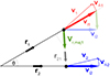Fig. 3.

Major infall model for galaxy 1: the radial infall velocity of galaxy 1 onto galaxy 2 can be determined from the projection of the radial infall velocity and the line-of-sight velocity of galaxy 2 onto the line-of-sight of galaxy 1. An analogous procedure yields the major infall model for galaxy 2. Due to the asymmetry of this model, both radial infall velocities need not be of the same size.

analogously for galaxy 2. Solving for |v_r, maji| for i = 1, 2, yields

$\begin{matrix} | v_{r, maj 1} | & = \frac{| v_{l 2} | cos θ - | v_{l 1} |}{{\bar{r}}_{2} cos θ - {\bar{r}}_{1}}, \end{matrix}$ $\begin{aligned} \left| \boldsymbol{v}_{\mathrm{r} , \mathrm{maj} 1} \right|&= \frac{\left| \boldsymbol{v}_{\mathrm{l} 2} \right| \cos \theta - \left| \boldsymbol{v}_{\mathrm{l} 1} \right|}{\overline{r}_2 \cos \theta -\overline{r}_1},\end{aligned}$ (37)

$\begin{matrix} | v_{r, maj 2} | & = \frac{| v_{l 1} | cos θ - | v_{l 2} |}{{\bar{r}}_{2} - {\bar{r}}_{1} cos θ} . \end{matrix}$ $\begin{aligned} \left| \boldsymbol{v}_{\mathrm{r} , \mathrm{maj} 2} \right|&= \frac{\left| \boldsymbol{v}_{\mathrm{l} 1} \right| \cos \theta - \left| \boldsymbol{v}_{\mathrm{l} 2} \right|}{\overline{r}_2 -\overline{r}_1 \cos \theta }. \end{aligned}$ (38)

For comparison, the generalised version of the major infall model is obtained by projecting Eq. (28) onto ${\hat{r}}_{i}$ $\hat{\boldsymbol{r}}_i$ :

$\begin{matrix} (v_{2} - v_{1}) \cdot {\hat{r}}_{i} = (| v_{r} | {\hat{r}}_{21} + | v_{t} | {\hat{r}}_{⊥ 21}) \cdot {\hat{r}}_{i}, i = 1, 2 . \end{matrix}$ $\begin{aligned} \left( \boldsymbol{v}_2 - \boldsymbol{v}_1 \right) \cdot \hat{\boldsymbol{r}}_i = \left( \left| \boldsymbol{v}_{\mathrm{r} }\right| \hat{\boldsymbol{r}}_{21} + \left| \boldsymbol{v}_{\mathrm{t} } \right| \hat{\boldsymbol{r}}_{\perp 21} \right) \cdot \hat{\boldsymbol{r}}_i \;, \quad i = 1,2. \end{aligned}$ (39)

Solving for |v_r|, we obtained

$\begin{matrix} | v_{r} | & = \frac{| v_{l 2} | cos θ - | v_{l 1} | + sin θ (| v_{⊥ 2} | - {\bar{r}}_{2} | v_{t} |)}{({\bar{r}}_{2} cos θ - {\bar{r}}_{1})}, i = 1 \end{matrix}$ $\begin{aligned} \left| \boldsymbol{v}_{\mathrm{r} } \right|&= \frac{\left| \boldsymbol{v}_{\mathrm{l} 2} \right| \cos \theta - \left| \boldsymbol{v}_{\mathrm{l} 1} \right| + \sin \theta \left( \left| \boldsymbol{v}_{\perp 2} \right| - \overline{r}_2 \left| \boldsymbol{v}_{\mathrm{t} } \right| \right)}{\left(\overline{r}_2 \cos \theta - \overline{r}_1 \right)}, \; i = 1\end{aligned}$ (40)

$\begin{matrix} \approx | v_{l 2} | - | v_{l 1} | + θ (| v_{⊥ 2} | - {\bar{r}}_{2} | v_{t} |), \end{matrix}$ $\begin{aligned}&\approx \left| \boldsymbol{v}_{\mathrm{l} 2} \right| - \left| \boldsymbol{v}_{\mathrm{l} 1} \right| + \theta \left( \left| \boldsymbol{v}_{\perp 2} \right| - \overline{r}_2 \left| \boldsymbol{v}_{\mathrm{t} } \right| \right),\end{aligned}$ (41)

$\begin{matrix} | v_{r} | & = \frac{| v_{l 2} | - | v_{l 1} | cos θ + sin θ (| v_{⊥ 1} | - {\bar{r}}_{1} | v_{t} |)}{({\bar{r}}_{2} - {\bar{r}}_{1} cos θ)}, i = 2 \end{matrix}$ $\begin{aligned} \left| \boldsymbol{v}_{\mathrm{r} } \right|&= \frac{\left| \boldsymbol{v}_{\mathrm{l} 2} \right| - \left| \boldsymbol{v}_{\mathrm{l} 1} \right| \cos \theta + \sin \theta \left( \left| \boldsymbol{v}_{\perp 1} \right| - \overline{r}_1 \left| \boldsymbol{v}_{\mathrm{t} } \right| \right)}{\left(\overline{r}_2 - \overline{r}_1 \cos \theta \right)}, \; i = 2\end{aligned}$ (42)

$\begin{matrix} \approx | v_{l 2} | - | v_{l 1} | + θ (| v_{⊥ 1} | - {\bar{r}}_{1} | v_{t} |) . \end{matrix}$ $\begin{aligned}&\approx \left| \boldsymbol{v}_{\mathrm{l} 2} \right| - \left| \boldsymbol{v}_{\mathrm{l} 1} \right| + \theta \left( \left| \boldsymbol{v}_{\perp 1} \right| - \overline{r}_1 \left| \boldsymbol{v}_{\mathrm{t} } \right| \right). \end{aligned}$ (43)

Thus, the major infall model is accurate for θ ≠ 0 and r_i ≠ 0 if

$\begin{matrix} i = 1 : | v_{⊥ 2} | = {\bar{r}}_{2} | v_{t} |, or i = 2 : | v_{⊥ 1} | = {\bar{r}}_{1} | v_{t} | . \end{matrix}$ $\begin{aligned} i = 1: \; \left| \boldsymbol{v}_{\perp 2} \right| = \overline{r}_2 \left| \boldsymbol{v}_{\mathrm{t} } \right|, \quad \mathrm{or} \quad i = 2: \; \left| \boldsymbol{v}_{\perp 1} \right| = \overline{r}_1 \left| \boldsymbol{v}_{\mathrm{t} } \right|. \end{aligned}$ (44)

Combining both equations to eliminate the unknown |v_t| yields Eq. (32) again. So, the conditions for over- or under-estimation of the true radial velocity are the same as for the minor infall.

A special case is |v_t| = 0, implying a purely radial infall, and |v_⊥i| = 0, i = 1, 2. Only considering one equation of Eqs. (40) and (42), this case yields a purely radial infall of one galaxy under a symmetry constraint that forces the perpendicular velocity of the other galaxy or the group centre to vanish (see Sect. 3).

2.5. Comparison and limits

The general versions of the infall models are easily related to each other via the different projections and it is obvious that both models are independent of a background cosmology. The minor infall model is best used when we do not have more information beyond θ, v_li, i = 1, 2. Since the model does not make any assumption about v_t and treats each galaxy of a pair equally, it is well suited for describing binary galaxies.

In contrast, the major infall model is best used for an ensemble of several galaxies. While it can also describe a pair, it requires information about the tangential and perpendicular components. The latter can be added via symmetry assumptions, readily testable in groups but hard to establish for binaries, with the Milky Way and Andromeda system being the only exception known so far, Benisty et al. (2022).

Replacing galaxy 2 with the centre of mass of the entire structure explains why the major infall model is asymmetric in the infalling objects. Any external impact, such as an accelerated cosmic expansion, will not generate additional angular momentum, increasing v_⊥2. Symmetry assumptions and a correspondingly well-sampled distribution of galaxies then allow us to describe groups and clusters robustly even over cosmic time.

Comparing Eqs. (34) and (37), or (38), their difference reads

$\begin{matrix} | v_{r, \min} | - | v_{r, maj 1} | = \frac{{\bar{r}}_{2} ({cos}^{2} θ - 1)}{{\bar{r}}_{2} cos θ - {\bar{r}}_{1}} (| v_{l 2} | {\bar{r}}_{1} - | v_{l 1} | {\bar{r}}_{2}), \end{matrix}$ $\begin{aligned} \left| \boldsymbol{v}_{\mathrm{r} , \mathrm{min} } \right| -\left| \boldsymbol{v}_{\mathrm{r} , \mathrm{maj} 1} \right| = { \tfrac{\overline{r}_2 \left( \cos ^2 \theta -1 \right)}{\overline{r}_2 \cos \theta - \overline{r}_1} \left( \left| \boldsymbol{v}_{\mathrm{l} 2} \right| \overline{r}_1 - \left| \boldsymbol{v}_{\mathrm{l} 1} \right| \overline{r}_2 \right)}, \end{aligned}$ (45)

and analogously for |v_r, maj2|. For r_i ≠ 0 and $v_{l 2} {\bar{r}}_{1} \neq v_{l 1} {\bar{r}}_{2}$ $\boldsymbol{v}_{\mathrm{l} 2} \overline{r}_1 \ne \boldsymbol{v}_{\mathrm{l} 1} \overline{r}_2$ , the infall models only agree for θ = 0 or θ = π. Thus, for small angles, as considered in prior work, both models coincide in the trivial relation up to small deviations:

$\begin{matrix} | v_{r, \min} | = | v_{r, maj 1} | = | v_{r, maj 2} | = | v_{r} | = | v_{l 2} | - | v_{l 1} | . \end{matrix}$ $\begin{aligned} \left| \boldsymbol{v}_{\mathrm{r} , \mathrm{min} } \right| = \left| \boldsymbol{v}_{\mathrm{r} , \mathrm{maj} 1} \right| = \left| \boldsymbol{v}_{\mathrm{r} , \mathrm{maj} 2} \right| = \left| \boldsymbol{v}_\mathrm{r} \right| = \left| \boldsymbol{v}_{\mathrm{l} 2} \right| - \left| \boldsymbol{v}_{\mathrm{l} 1} \right|. \end{aligned}$ (46)

In addition, for θ = π, both infall models coincide again. For 0 < θ < π, the difference can be positive or negative depending on the relations between all quantities involved. Since both models can over- or under-estimate the true radial infall velocity based on Eq. (32), we cannot decide which model is closer to the true radial component without additional information or assumptions.

3. From binaries to groups and clusters

The approaches in Karachentsev & Kashibadze (2006) rely on spherical symmetry and require the member galaxies to sample the total spherical mass distribution well. To investigate the impact of each assumption, let the centre of the total mass distribution (stellar, gaseous, dark mass) be r_cm and its total velocity $v_{cm} = d r_{cm} / d t$ $\boldsymbol{v}_{\mathrm{cm}} = \rm{d}\boldsymbol{r}_{\mathrm{cm}}/\rm{d}t$ . For n member galaxies sampling this mass-density profile, their centre of mass and its velocity are given by

$\begin{matrix} r_{cg} = \frac{1}{M_{g}} \sum_{i = 1}^{n} m_{i} r_{i}, v_{cg} = \frac{1}{M_{g}} \sum_{i = 1}^{n} m_{i} v_{i}, \end{matrix}$ $\begin{aligned} \boldsymbol{r}_{\mathrm{cg} } = \frac{1}{M_{\mathrm{g} }} \sum \limits _{i = 1}^{n}m_i \boldsymbol{r}_i \;, \quad \boldsymbol{v}_{\mathrm{cg} } = \frac{1}{M_{\mathrm{g} }} \sum \limits _{i = 1}^{n}m_i \boldsymbol{v}_i, \end{aligned}$ (47)

where M_g is the mass of all galaxies and we assumed that the galaxies move non-relativistically. While M_g is known when the mass-to-light ratio of the galaxies is known, the total mass of the structure, M, remains unknown, for instance, including a galaxy-cluster-scale dark-matter halo in which the galaxies are moving, so M ≥ M_g. The galaxies are a representative sample if, at least, r_cm = r_cg and v_cm = v_cg. These quantities need not agree generally, for instance, for a very small number of galaxies, in merger scenarios, or if the dark matter distribution is not well traced by the luminous matter. For r_i = r_cm − r_cm i and v_i = v_cm − v_cm i, the total momentum with respect to the observer is

$\begin{matrix} P = M_{g} v_{cm} - \sum_{i = 1}^{n} m_{i} v_{cm i} . \end{matrix}$ $\begin{aligned} \boldsymbol{P} = M_\mathrm{g} \boldsymbol{v}_\mathrm{cm} - \sum \limits _{i = 1}^{n} m_i \, \boldsymbol{v}_{\mathrm{cm} \, i}. \end{aligned}$ (48)

If r_cm = r_cg, the sum vanishes. Assuming a spherically symmetric structure on a homogeneous and isotropic background, v_cm reduces to the cosmic velocity along the observer’s line of sight. Without these assumptions, P is not well constrained even for n ≫ 2 due to the unknown perpendicular and tangential parts.

The total angular momentum with respect to the observer is

$\begin{matrix} L = \sum_{i = 1}^{n} m_{i} r_{i} \times v_{i} \equiv | L_{1} + L_{2} - L_{3} - L_{4} | {\hat{r}}_{cm} \times {\hat{r}}_{⊥ cm} . \end{matrix}$ $\begin{aligned} \boldsymbol{L} = \sum \limits _{i = 1}^{n} m_i \, \boldsymbol{r}_i \times \boldsymbol{v}_i \equiv \left| \boldsymbol{L}_1 + \boldsymbol{L}_2 - \boldsymbol{L}_3 - \boldsymbol{L}_4 \right| \, \hat{\boldsymbol{r}}_{\mathrm{cm} } \times \hat{\boldsymbol{r}}_{\perp \mathrm{cm} } . \end{aligned}$ (49)

With the relations in Sect. 2.1, the four parts read

$\begin{matrix} | L_{1} | & = | \sum_{i = 1}^{n} m_{i} r_{cm} \times v_{⊥ cm} | = M_{g} | r_{cm} | | v_{⊥ cm} |, \end{matrix}$ $\begin{aligned} \left| \boldsymbol{L}_1 \right|&= \Big | \sum \limits _{i = 1}^{n} m_i \, \boldsymbol{r}_{\mathrm{cm} } \times \boldsymbol{v}_{\perp \mathrm{cm} } \Big | = M_{\mathrm{g} } \left| \boldsymbol{r}_{\mathrm{cm} } \right| \left| \boldsymbol{v}_{\perp \mathrm{cm} } \right|,\end{aligned}$ (50)

$\begin{matrix} | L_{2} | & = | \sum_{i = 1}^{n} m_{i} r_{cm i} \times v_{⊥ cm i} | = \sum_{i = 1}^{n} m_{i} | r_{cm i} | | v_{t i} |, \end{matrix}$ $\begin{aligned} \left| \boldsymbol{L}_2 \right|&= \Big | \sum \limits _{i = 1}^{n} m_i \, \boldsymbol{r}_{\mathrm{cm} \, i} \times \boldsymbol{v}_{\perp \mathrm{cm} \, i} \Big | = \sum \limits _{i = 1}^{n} m_i \left|\boldsymbol{r}_{\mathrm{cm} \, i} \right| \left| \boldsymbol{v}_{\mathrm{t} \, i} \right|,\end{aligned}$ (51)

$\begin{matrix} | L_{3} | & = | \sum_{i = 1}^{n} m_{i} r_{cm i} \times v_{cm} |, \end{matrix}$ $\begin{aligned} \left| \boldsymbol{L}_3 \right|&= \Big | \sum \limits _{i = 1}^{n} m_i \, \boldsymbol{r}_{\mathrm{cm} \, i} \times \boldsymbol{v}_{\mathrm{cm} } \Big |,\end{aligned}$ (52)

$\begin{matrix} = \sum_{i = 1}^{n} m_{i} (| v_{⊥ cm} | (| r_{cm} | - | r_{i} | cos θ_{i}) + | v_{l cm} | | r_{i} | sin θ_{i}), \end{matrix}$ $\begin{aligned}&= \sum \limits _{i = 1}^{n} m_i \, \Big ( \left| \boldsymbol{v}_{\perp \mathrm{cm} } \right| (\left| \boldsymbol{r}_{\mathrm{cm} } \right| - \left|\boldsymbol{r}_i \right| \cos \theta _i) + \left| \boldsymbol{v}_{\mathrm{l} \, \mathrm{cm} } \right| \left| \boldsymbol{r}_i \right| \sin \theta _i \Big ),\end{aligned}$ (53)

$\begin{matrix} | L_{4} | & = | \sum_{i = 1}^{n} m_{i} r_{cm} \times v_{cm i} | = - \sum_{i = 1}^{n} m_{i} | v_{r i} | | r_{cm} | {\bar{r}}_{i} sin θ_{i} . \end{matrix}$ $\begin{aligned} \left| \boldsymbol{L}_4 \right|&= \Big | \sum \limits _{i = 1}^{n} m_i \, \boldsymbol{r}_{\mathrm{cm} } \times \boldsymbol{v}_{\mathrm{cm} \, i} \Big | = - \sum \limits _{i = 1}^{n} m_i \, \left|\boldsymbol{v}_{\mathrm{r} \, i} \right| \left| \boldsymbol{r}_{\mathrm{cm} } \right| \overline{r}_i \sin \theta _i. \end{aligned}$ (54)

For an arbitrary observer in a homogeneous and isotropic universe, there is no reason for a total angular momentum to exist, such that |L| = 0 for an isolated single structure, supported by observations Hawking (1969), Saadeh et al. (2016). As assumed in Karachentsev & Kashibadze (2006), if r_cm = r_cg, L₃ and L₄ vanish. From the remaining |L₁| = −|L₂|, we obtained

$\begin{matrix} | v_{⊥ cm} | + \frac{m_{j}}{M_{g}} \frac{| r_{cm j} |}{| r_{cm} |} | v_{t j} | = - \sum_{i = 1, i \neq j}^{n} \frac{m_{i}}{M_{g}} \frac{| r_{cm i} |}{| r_{cm} |} | v_{t i} |, \end{matrix}$ $\begin{aligned} \left| \boldsymbol{v}_{\perp \mathrm{cm} } \right| + \frac{m_j}{M_\mathrm{g} } \frac{\left| \boldsymbol{r}_{\mathrm{cm} \, j} \right|}{\left| \boldsymbol{r}_{\mathrm{cm} }\right|} \left| \boldsymbol{v}_{\mathrm{t} \, j} \right| = - \sum \limits _{i = 1, i\ne j}^{n} \frac{m_i}{M_\mathrm{g} } \frac{\left| \boldsymbol{r}_{\mathrm{cm} \, i} \right|}{\left| \boldsymbol{r}_{\mathrm{cm} } \right|} \left| \boldsymbol{v}_{\mathrm{t} \, i} \right|, \end{aligned}$ (55)

taking galaxy j outside the sum, assuming it falls onto a structure of n − 1 galaxies. Then, we required n ≫ 1 and a spherically symmetric structure in which the right-hand side of Eq. (55) averages to zero. Eq. (55) amounts to $| v_{⊥ cm} | = λ {\bar{r}}_{cm} | v_{t j} |$ $\left| \boldsymbol{v}_{\perp \mathrm{cm}} \right| = \lambda \overline{r}_{\mathrm{cm}} \left| \boldsymbol{v}_{\mathrm{t} \, j} \right|$ compared to Eq. (44). However, only the projection of v_t on the observer’s sky can be observed. So we may absorb λ into the definition of v_t for the infall model and study its degeneracies with the projection angle on the observer’s sky in a subsequent step. The major infall model then relates |v_t j| to |v_⊥cm|.

Alternatively, all galaxies are in the spherically symmetric structure on the right-hand side of Eq. (55), hence |v_⊥cm| = 0. Inserting the latter into Eqs. (40) and (42), solving for |v_⊥i| and |v_t i| yields

$\begin{matrix} | v_{⊥ i} | = 0 \lor θ = 0 \lor θ = π / 2 \lor θ = π . \end{matrix}$ $\begin{aligned} \left| \boldsymbol{v}_{\perp i} \right| = 0 \quad \vee \quad \theta = 0 \quad \vee \quad \theta = \pi /2 \quad \vee \quad \theta = \pi . \end{aligned}$ (56)

Hence, the |v_t i| do not need to vanish, so that the minor infall model is equally suitable to be used in this case.

The trivial case, |v_⊥cm| = |v_t j| = 0, mentioned in Sect. 2.4 is obtained for a purely radial infall, |v_t j| = 0 either for galaxy j onto a spherical structure, or even ∀j = 1, …n, both yielding |L₁| = |L₂| = 0. Deviations from Eq. (44) can already arise from |L₂| due to a less symmetric structure or insufficient sampling n, apart from asymmetries between r_cm and r_cg causing L₃ and L₄ to be non-zero.

Rewriting Eq. (49) in terms of all |v_r, maj i|, we used Eq. (40) with a λ-factor in front of |v_t i| as above but without the mass ratio, and θ_i ≠ 0 to obtain

$\begin{matrix} | L_{1} + L_{2} | = \sum_{i = 1}^{n} \frac{m_{i}}{sin θ_{i}} | r_{cm} | ({\bar{r}}_{cm} cos θ_{i} - {\bar{r}}_{i}) (| v_{r i} | - | v_{r, maj i} |) . \end{matrix}$ $\begin{aligned} \left| \boldsymbol{L}_1 + \boldsymbol{L}_2 \right| = \sum \limits _{i = 1}^{n} \frac{m_i}{\sin \theta _i} \left| \boldsymbol{r}_{\mathrm{cm} } \right| (\overline{r}_{\mathrm{cm} } \cos \theta _i - \overline{r}_i) \left( \left| \boldsymbol{v}_{\mathrm{r} \, i} \right| - \left| \boldsymbol{v}_{\mathrm{r,maj} \, i} \right| \right). \end{aligned}$ (57)

For θ_i = 0, Eq. (46) holds without giving a contribution to Eq. (57). Detailed in Sect. 2.4, the major infall model may over- or under-estimate |v_r|, such that any |L| ≠ 0 depends on the sum of deviations for all galaxies, which, in turn, depends on the symmetry of the structure. Since the minor infall does not include |v_t|, Eq. (57) only relates the major infall model to the true radial velocity.

4. Application to simulated structures

As a proof-of-principle test, we applied the infall models to the snapshot of cosmic structures at z = 0 in the Illustris-3 simulation, Vogelsberger et al. (2014) and Nelson et al. (2015), which is based on our cosmological concordance model. While Sect. 2 tackles binaries and groups with more than two members alike, Benisty et al. (2025a) will provide more details about infall models for binaries, so we focussed on groups here.

From all of the halos identified by the friends-of-friends clustering, we selected those with a galaxy-group-scale mass of m_halo > 10¹² M_⊙/h with the dimensionless Hubble constant, h = 0.704. To ensure that all halos and their subhalos are well sampled, we considered halos with a minimum number of particles larger than 100 and subhalos with at least 20 particles. While Illustris-3 is the least resolved simulation compared to Illustris-1 and 2, its halo and subhalo catalogues list the centre of mass position of the halos and subhalos in addition to the position of the most bound particle. The additional information allowed us to select relaxed halos and non-merging subhalos: we required both comoving positions to differ by less than 10 ckpc/h for halos and subhalos. Yet, this is just one option among many, as is detailed in Zjupa & Springel (2017) and references therein.

We furthermore required that the halos be isolated, meaning we only investigated halos without any neighbouring halos within the radius of their own zero-velocity surface r₀ ≡ ∥r₀∥₂ plus the maximum r₀ of all halos in the simulation. To calculate r₀, we used the relation derived in Peirani & de Freitas Pacheco (2006)

$\begin{matrix} m_{0} \approx 4.1 \times 10^{12} h^{2} {(\frac{r_{0}}{1 Mpc})}^{3} M_{⊙} \end{matrix}$ $\begin{aligned} m_{0} \approx 4.1 \times 10^{12} h^2 \left(\frac{r_0}{1\,\mathrm{Mpc}}\right)^3\,M_\odot \end{aligned}$ (58)

for r₀, setting the mass enclosed in this radius m₀ equal to the simulated halo mass. For our final set of 344 halos, r₀ ∈ [0.89,2.00] Mpc. As we assumed that the origin of the simulation is a random position in the snapshot, we placed the observer at this position. Fig. 4 shows the distribution of physical distances versus the halo masses for the 344 selected halos.

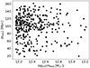Fig. 4.

Physical distances from an observer at the origin to the centre of mass of 344 isolated, relaxed halos versus their halo masses in the z = 0-snapshot of Illustris-3. In the notation of Sect. 3, |r_halo|≡|r_cm|.

For the selection of subhalos, we pursued two approaches: first, we loaded all subhalos that are gravitationally bound to their parent halo as indicated in the subhalo catalogue. Second, to study the behaviour of the infall models in the Hubble flow around the structures, we selected all subhalos that are within a sphere of 1.5 r₀. For the first approach, the number of subhalos per halo is n_sub ∈ [1,38] with a total of 1476 bound subhalos, for the second n_sub ∈ [1,92] with a total of 5036 subhalos.

After the selection process, we converted all comoving quantities to physical ones. This required us to add a Hubble flow to the simulated velocities of all halos and subhalos v_simj as

$\begin{matrix} v_{j} = v_{sim j} + H_{0} r_{j} . \end{matrix}$ $\begin{aligned} \boldsymbol{v}_j = \boldsymbol{v}_{\mathrm{sim} j} + H_0 \boldsymbol{r}_j. \end{aligned}$ (59)

As a result, we obtained the final data on which we performed our infall-model tests.

While the position of the most bound particle is usually used to locate halos and subhalos, we employed the centre of mass coordinates instead. This is motivated by the derivations of Sect. 3. Based on our selection criteria, the differences between using the most bound particle or the centre of mass are minor. Moreover, using the most bound particle, numerical instabilities occur for most of the central subhalos when their most bound particle has exactly the same position as the most bound particle of the parent halo, such that no infall models can be calculated for it.

At first, we tested the accuracy of the minor and major infall models to reconstruct the radial velocity. Since the halos are at distances beyond 18 Mpc, ∥r_cmj∥₂ ∈ [0,3] Mpc with ∥θ∥₂ ∈ [0,7.4] deg and thus small compared to the angles of objects in our cosmic neighbourhood investigated by Karachentsev & Kashibadze (2006), Karachentsev & Nasonova (2010), and others. Thus, the small-angle approximation discussed in Sect. 2 should hold, implying that the sin θ-terms in Eqs. (22), (40), and (42) are suppressed.

Yet, Fig. 5 shows a different picture: in Fig. 5 (left), we plotted the infall velocities according to Eqs. (34), (37), and (46) of all 5036 subhalos, bound and unbound, onto their parent-halo centre versus the true radial velocity. The approximation of Eq. (46) shows a similar scatter as the minor infall model, supporting the statement in Sect. 2.5 that it is a good approximation of the latter for the small angles at least out to 7.4 deg. Both models have a limited spread, such that a linear fit |v_infj|=m_v|v_rj| can be calculated together with its 1-σ confidence bounds b_v. For the minor infall model we obtained m_v = 0.43, b_v = 81.06 km/s, for the approximation by Eq. (46) m_v = −0.04, b_v = 153.39 km/s. Comparing Eqs. (34) and (37), the spread of the major infall velocity is larger, which is caused by the fact that the major infall model is a ratio and the denominator can have a small absolute value. Fitting a line to this data, yields m_v = 1.01, but also b_v = 5578.32 km/s. As Fig. 5 (left) only shows infall velocities up to an absolute value of 4000 km/s, not all major-infall velocities are in the plot. Restricting the line fits to consider bound subhalos only, the values only change marginally.

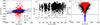Fig. 5.

Left: Reconstructed infall velocities by Eqs. (34), (37), and (46) for all subhalos (bound in dark colours, Hubble-flow subhalos in light colours) onto their parent-halo centre versus the true radial velocity by Eq. (22). Linear fits with 1-σ confidence bounds to the point clouds of the minor infall model and the velocity-difference approximation are shown in blue and grey, respectively. The fit for the major infall is not shown as its confidence bound covers the entire plot. Centre: Perpendicular velocities of all subhalos versus their distance to the observer (bound in black, Hubble-flow subhalos in grey). Only the six subhalos in the Hubble flow marked in blue have a tangential velocity close to zero. In the notation of Sect. 3, |r_subhalo|≡|r_j|. Right: Absolute value of the tangential velocity of all subhalos (bound in dark colours, Hubble-flow subhalos in light colours) versus their radial velocity. Only 337 subhalos with radial velocity close to zero also have a tangential velocity close to zero (marked in blue), while 3575 subhalos have a larger tangential velocity than radial one (marked in red).

To investigate the source of the deviations from the true radial velocity, we plotted the perpendicular velocities for each subhalo versus its physical distance to us in Fig. 5 (centre). As the plot shows, there is no trend of vanishing perpendicular velocities visible, although they maximally amount to 34% of the line-of-sight velocities and are therefore much smaller. Only six subhalos in the Hubble flow have perpendicular velocities smaller than 10 km/s, which can be interpreted as conservatively compatible with zero (see for instance Kim et al. 2020). So even though sin θ is small, the perpendicular velocities multiplied by the normalised distances compensate for the small angle and therefore yield a non-negligible contribution to the last term of the radial infall velocity in Eq. (22). This is in contrast to the assumptions made in Karachentsev & Kashibadze (2006) that the peculiar velocities of the galaxies are small compared to the line-of-sight velocities subject to the Hubble flow.

Since the perpendicular velocities are not negligible, we plotted the absolute value of the tangential velocity for all subhalos in Fig. 5 (right). The plot shows a similar result. Only 337 subhalos out of 5036 subhalos have a tangential velocity that is smaller than 10 km/s. Further investigating the properties of these subhalos, we discovered that 309 approximately obey Eq. (30) with θ ≈ 0, even |r_cmj|≈0 and a maximum ||v_⊥cm − v_⊥j||₂ = 12 km/s. These subhalos are the central subhalos close to the centre of the parent halo. For three additional bound halos and 25 in the Hubble flow, another fine-tuning reduces ||v_tj||₂ < 10 km/s by chance. The remaining 4699 subhalos thus have a non-negligible tangential velocity, for 3575 of those even ||v_tj||₂ > ||v_rj||₂ holds. In summary, 93% of all tangential velocities are not negligible and 71% of all ||v_tj||₂ exceed ||v_rj||₂.

Based on these findings and supported by Eq. (30), it is not sufficient to restrict the application of the infall models to galaxies that are in front and behind the cluster centre with θ ≈ 0 in order to reduce the impact of the tangential velocity, as stated in Karachentsev & Nasonova (2010). Moreover, Karachentsev & Kashibadze (2006) studied the impact of v_tj by simulating a distributions of tangential velocities as a Gaussian amplitude with mean 70 km/s and standard deviation of 30 km/s combined with a uniform distribution in the orientation. While this might be a realistic choice of parameters for the close-by low-mass cosmic structures they investigated, the result does not hold in general, as Fig. 5 (right) reveals.

At last, we investigated the statement made in Kim et al. (2020) that the true radial velocities of the Virgo cluster are expected to lie between the major and minor infall model estimates, which is not supported by the theoretical derivations in Sect. 2.5. Out of 5036 subhalos in our data set, only 34%, meaning 1707, fulfill this condition. Since Virgo is at 16.5 Mpc from us as observers and has m₀ ≈ 6 × 10¹⁴ M_⊙ according to Kim et al. (2020), it is out of the distance and mass range covered by our halo selection. However, the infall models are based on a purely geometrical kinematics construct, so that it is very likely that our findings also apply to the Virgo cluster. To support this claim, Fig. 6 (left, centre) shows there is no correlation between the radial velocity of a subhalo and its parent halo mass or the physical distance of its parent halo to the observer. Marking all subhalos whose radial velocity lies between the minor and major infall velocity in blue, we also read off Fig. 6 (left, centre) that there is no correlation for those cases, either. Analogously to Fig. 7 in Kim et al. (2020), we plotted the Hubble flow around the centre of our most massive halo in Fig. 6 (right) to show that the true radial velocity need not lie between the minor and major infall velocity. For this halo, m_halo = 1.64 × 10¹³ M_⊙ corresponding to r₀ = 2.00 Mpc. We counted 38 bound subhalos and 54 in the Hubble flow out to 1.5 r₀, amounting to 92 subhalos in total. For those, 14 out of 38 bound subhalos have a radial velocity between the minor and major infall velocities, and 31 out of the 54 in the Hubble flow. Hence, only 49% of all subhalos fulfil this constraint. (For the second most massive halo with a total of 43 subhalos (20 bound, 23 in the Hubble flow), the ratio is only 30%.)

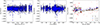Fig. 6.

Left: Radial velocity of all 5036 subhalos onto their parent halo versus the mass of their parent halo, highlighted in blue are those subhalos whose radial velocity lies between the minor and major infall velocity (dark colours mark bound halos, light colours mark subhalos in the Hubble flow). Centre: Same as the previous plot, but depending on the distance of the parent halo to the observer instead of the parent-halo mass. Right: Hubble-flow diagram for the most massive halo in our halo set to be compared with Fig. 7 of Kim et al. (2020). The major and minor infall velocities can be compared to the true radial infall velocity (dark colours mark bound halos, light colours mark subhalos in the Hubble flow), squared markers indicate which radial velocities lie between the minor and major infall velocities.

While the infall model velocities themselves cannot constrain the radial velocity in a robust way, Fig. 7 shows that the velocity dispersions are more suitable to constrain the true velocity dispersion. The plot shows the velocity dispersions of the bound subhalos for all 109 halos containing at least five bound subhalos. With only a few exceptions, the minor infall model systematically underestimates the true velocity dispersion, and the major infall model, even with a larger spread, systematically overestimates it. The infall velocity of Eq. (46) seems to yield the closest match to the true velocity dispersion. However, this result may not hold for cosmic structures at closer distances to the observer with larger θ. Fitting a line with a 1-σ confidence bound to all three velocity dispersion estimates, we obtained for the minor infall model m_σ = 0.58, b_σ = 25.78 km/s, for the major infall model m_σ = 3.48, b_σ = 208.36 km/s, and for the velocity difference model of Eq. (46) m_σ = 0.99, b_σ = 47.06 km/s. In order to discard the quasi numerically unstable major infall velocities for which |r_cmj|≈0, we cut the absolute value at 3000 km/s, omitting 2%, 31 out of 1476, bound subhalos. Hence, the plotted major-infall velocity dispersions are marginally lower compared to including these outliers. For a set of observed galaxy groups in the same mass and distance range as our simulated selection, the parameters from the line fits could also be used to calibrate the velocity dispersions as obtained from the data in order to alleviate the model-based biases (see Sect. 5 for an example).

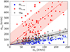Fig. 7.

Velocity dispersions of bound subhalos for halos containing at least five bound subhalos j = 1, …, 109, calculated based on the minor and major infall models, as well as the infall velocity approximated by Eq. (46).

Given these findings, any quantity which is dependent on the velocity dispersion can have a robust upper and lower bound based on the velocity dispersions of the minor and major infall model, or even a strong estimate based on the velocity dispersion of Eq. (46), if the cosmic structure is far away enough from the observer. One example of such a quantity is the virial mass. In contrast to this, any quantity which is dependent on the infall velocity itself may not have a robust upper and lower bound when the infall models are employed. One example is the m₀- and r₀-estimates based on Hubble-flow fits, as performed in Kim et al. (2020). It still remains an open question in how far a Hubble-flow fit to the minor and major infall models robustly yields upper and lower bounds on m₀ and r₀. Since this may also depend on the specific version of the Hubble-flow fitting function, this analysis is beyond the scope of this work.

At last, we investigated the assumptions made in Sect. 3 that motivate the major infall model. The Illustris-3 simulation has too low a resolution that we could have tested the impact of offsets between dark and luminous matter, i.e. whether the centre of light of the observed galaxies coincides with their centre of their mass and then infers the centre of mass of the galaxy cluster correctly. So we could only analyse the ideal case, assuming we knew the centre of mass of the member galaxies of a cluster. Fig. 8 (left) shows that the offset between the centre of mass of a halo and the centre of mass position of all its bound subhalos is very small compared to the halo extent, r₀. Thus, r_cm = r_cg can be assumed for our halo selection.

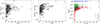Fig. 8.

Left: Difference between the centre of mass of the parent halo and the centre of mass of the bound subhalos calculated as the mass-weighted sum of all their centre-of-mass positions versus the number of bound subhalos. The difference in the centre-of-mass positions is scaled to the zero-velocity radius of the halo for comparison. Centre: Total angular momentum as given by Eq. (49) versus the number of bound subhalos. Right: Individual components of the angular momentum given by Eqs. (50)–(54) with respect to the total one versus the number of bound subhalos.

Next, we determined the total angular momentum of a halo from all bound subhalos as defined by Eq. (49) and plotted its value against the number of bound subhalos in Fig. 8 (centre). Obviously, the angular momenta of the halos are far from vanishing. To sort the four individual parts of L as defined by Eqs. (50)–(54), we scaled each of them to the total angular momentum and plotted them in Fig. 8 (right). As can be read off Fig. 8 (right), the largest contribution to L comes from the angular momentum of the halo with respect to the observer. Hence, a vanishing overall angular momentum may be applicable to a large ensemble of halos that sample the volume around the observer well. However, for individual galaxy groups and clusters, this assumption does not hold. Only the assumption that the angular momentum within the cosmic structure L₂ is negligible compared to L₁ is true to a good approximation for our selected halos. More interestingly, the contributions of L₃ and L₄ are generally larger then the one of L₂, even for the small offsets between the halo centre of mass and the centre of mass inferred from its bound subhalos. So we concluded that the major infall model might be motivated by the derivations in Sect. 3, yet, the assumptions made to arrive at Eqs. (37) and (38) do not hold. Nevertheless, as we showed above, it is still a useful model to obtain an upper limit on the true radial velocity dispersion.

5. Application to the M81 group

After investigating the validity and limits of the infall-model assumptions with simulations, we applied the infall models to observations of the M81 group, whose Hubble flow was analysed in Karachentsev & Kashibadze (2006). We employed the recent data of M81 member galaxies, detailed in Müller et al. (2024). While there are more member galaxies known by now, we restricted our sample to the 21 of Müller et al. (2024), as listed in Table A.1, because they based their collection on a comparably homogeneous data set to avoid self-inconsistencies due to potential biases caused by using various observational methods together. As Müller et al. (2024) did not list the line-of-sight velocities and distances of M81 and M82, we added them from the same data base as used by Müller et al. (2024), Karachentsev et al. (2013).

Before we applied the infall models to the M81 group observables, we re-used the Illustris-3 simulation to select halos that have similar properties as those inferred from observations of the M81 group. This helps to understand the large spread of the major-infall velocity dispersion in the Hubble flow around the M81 group that Karachentsev & Kashibadze (2006) discovered. It also gives an insight into the behaviour of the infall models at local-universe distances and we could compare the simulated velocity dispersion values with those from the observations.

5.1. M81-group-like simulated structures

Similarly as in Sect. 4, we selected halos and subhalos from Illustris-3 that contain at least 30 and 20 particles, respectively. Based on the estimates of r₀ ≈ 1 Mpc for the M81 group in Karachentsev & Kashibadze (2006) and given that its environment has further infalling structures at a distance of about 1 Mpc (Chiboucas et al. 2013), we selected halos that do not have any other halo within 2 r₀ from their centre of mass. In addition, we required that the total halo mass m_halo ∈ [0.5,5.0] × 10¹² M_⊙, based on the Hubble-flow estimate of Karachentsev & Kashibadze (2006) that m_M81 ≈ 10¹² M_⊙. The halo should also contain at least six subhalos, as the data by Müller et al. (2024) contains 11 galaxies inside what is assumed to be the second turn-around radius of 230 kpc and we allowed for some fluctuations. Since the M81 group has three strongly interacting galaxies in its centre, M81, M82, and NGC 3077 and seems to be a merging group, we allowed a maximum offset between the centre of mass of the halo and the position of its most bound particle to be 100 kpc because this is the range of relative distances of the three interacting galaxies (see also Table A.1). The position of the centre of mass of the halo is used in the following as the distance to the halo. For the subhalos, we did not set any limits on their relaxation to account for their potential interactions and employed the position of their most bound particle as their position.

After selecting all halos and bound subhalos fulfilling these criteria, we also collected all subhalos around the halo out to 1.5 r₀ for the Hubble-flow analysis. Next, we set the observers’ position with respect to each halo such that their distance to the centre of mass of the halo is 3.7 Mpc and their relative velocity is –38 km/s, which corresponds to the velocity by which M81 is approaching us as observers.

Under these conditions, we obtained 281 halos to analyse. They contain a total of 2099 bound subhalos and 5938 out to 1.5 r₀ with n_subhalo ∈ [6,14] bound subhalos per halo and n_subhalo ∈ [7,127] out into the Hubble flow. Fig. 9 shows the same plots as in Fig. 5 for the new halo selection. Compared to Fig. 5, the peculiar velocities of the galaxies play a larger role here, as they cause larger deviations between the infall models and the true radial velocity (left). The perpendicular velocities exceed the line-of-sight velocities for 91% of all subhalos (92% of the bound ones) and are only compatible with zero in 2% of all cases (5% of the bound ones). Considering the tangential velocities, only 2% of all subhalos (6% of the bound ones) have such a component compatible with zero with a trend of jointly having a small radial velocity, similarly to the one observed in Fig. 5. However, 87% of all tangential velocities exceed the absolute value of the radial component and 89% out of all tangential velocities of bound subhalos. On the whole, the results obtained for the infall models applied to more massive halos at larger distances are also found for less massive halos at smaller distances. Even less subhalos fulfil the requirements of the infall models as stated in Karachentsev & Kashibadze (2006) because the impact of the peculiar velocities on top of the cosmic expansion is stronger at smaller distances from the observer. 695 (33%) of the bound subhalos have a radial velocity between the minor and major infall velocities, similarly, 1905 (32%) of all subhalos into the Hubble flow fulfil this criterion. This is approximately the same ratio as for the far-away, more massive halos of Sect. 4.

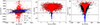Fig. 9.

Same as Fig. 5 but for the 281 M81-group-like halos. From all 5938 subhalos out to 1.5 r₀, 125 have a perpendicular velocity compatible with zero, 5427 have one that is larger than their line-of-sight velocity. For the bound subhalos, the numbers are 114 and 1925 out of 2099, respectively. 132 out of 5938 subhalos have a tangential velocity compatible with zero, for 5190, the tangential velocity exceeds the absolute value of the radial one. For the bound halos, the numbers are 118 and 1870, respectively.

5.2. Evaluation of observations and comparison

Many data points listed in Table A.1 lack proper measurement uncertainties. Thus, we took the heliocentric velocity components without accounting for their uncertainties to calculate the infall-model velocities and velocity dispersions of the member galaxies with respect to M81 as the centre for the infall. We then compared their results to those obtained by the simulation set up in Sect. 5.1, which amounts to the most direct comparison between observables and simulations possible. Fig. 10 (left) shows the infall-model velocities and the velocity according to Eq. (46) for the individual member galaxies. As we read off the plot, the spread in the infall velocities and even the large deviation between the infall velocity of Eq. (46) and the other infall models for many M81-group members resembles the findings of the simulations of Sect. 5.1, even though the simulated structures may not fully represent the characteristics of the M81 group.

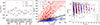Fig. 10.

Left: Infall-model velocities defined in Eqs. (34), (37), and (46) for each member of the M81 group (see Table A.1 for details on the data). Centre: Velocity dispersions of the infall models and the approximation of Eq. (46) of the bound subhalos in the simulation set up in Sect. 5.1 (same as Fig. 7) for j = 1, …, 281 halos. Dotted lines mark the velocity dispersions as determined for the M81 group members of Table A.1. Right: Ratios of absolute values of angular momenta as given by Eqs. (50)–(54) with respect to the total angular momentum (same as Fig. 8, right).

In Fig. 10 (centre), we applied the infall models to the bound subhalos of the M81-group-like simulated halos and plotted their velocity dispersions. Fitting lines with 1-σ confidence bounds to the data points, we found for the minor infall model m_σ = 0.53, b_σ = 22.21 km/s, for the approximation by Eq. (46) m_σ = 1.03, b_σ = 37.31 km/s, and for the major infall model m_σ = 4.01, b_σ = 254.60 km/s³. Thus, we found similar results as for the halo selection of Sect. 4.

The dotted lines in Fig. 10 (centre) are the velocity dispersions of the M81 group calculated for the heliocentric velocities, v_hel, of all members as listed in Table A.1. We obtained from

$\begin{matrix} the minor infall : σ_{r, \min} & = 96 km / s, \end{matrix}$ $\begin{aligned} \mathrm{the~minor~infall}: \sigma _{\mathrm{r,min}}&= 96\,\mathrm{km}/\mathrm{s},\end{aligned}$ (60)

$\begin{matrix} the major infall : σ_{r, maj} & = 564 km / s, \end{matrix}$ $\begin{aligned} \mathrm{the~major~infall}: \sigma _{\mathrm{r,maj}}&= 564\,\mathrm{km}/\mathrm{s},\end{aligned}$ (61)

$\begin{matrix} (46) : σ_{r, Δ v_{l}} & = 102 km / s . \end{matrix}$ $\begin{aligned} (46): \sigma _{\mathrm{r},\Delta \mathrm{v}_{\mathrm{l}}}&= 102\,\mathrm{km}/\mathrm{s}. \end{aligned}$ (62)

Often, heliocentric velocities are corrected for the motion of the sun with respect to a reference frame at larger scales. For the M81 group, which is a neighbour of the Local Group, Karachentsev et al. (2013) also gave all velocities of M81 members in the Local-Group-centroid frame, thus correcting for the solar motion within the Local Group (see Appendix A for details). Using these velocities given by v_LG in Table A.1, we obtained σ_r, min = 97 km/s, σ_r, maj = 631 km/s, and σ_{r, Δv_l} = 102 km/s. Thus, given the size of the 1-σ bounds on the simulated set of M81-like groups, the impact of this correction is likely to be absorbed in these bounds.

Yet, it remains questionable if this correction is reasonable to apply because it breaks the direct comparison to simulations, in which no such corrections are considered. The Local-Group centroid is further moving with respect to larger scales, as is M81 and additional corrections may need to be considered. The infall models also assume that the unobserved velocity components are fine-tuned and transforming into one from the above mentioned reference frames does not necessarily match these conditions. Moreover, the heliocentric velocities correspond to us as observers and have the tightest error bars, while transformations into other reference frames, like the Local-Group centroid frame, accumulate additional uncertainties and model assumptions, such as the uncertainties from the proper motion of M31 (see van der Marel et al. 2019 and Salomon et al. 2021), the Local-Group mass ratio (Karachentsev et al. 2009), and that the dark matter is concentrated around the Milky Way and Andromeda (Benisty & Mota 2025).

Assuming the M81 group to be a typical group obeying the average trends of the fitted lines, we read off the most likely radial velocity for all three approximations of Eqs. (60)–(62) from Fig. 10 (centre) as outlined to be a possible bias-correction method in Sect. 4:

$\begin{matrix} minor infall : σ_{r} & = (180 \pm 42) km / s, \end{matrix}$ $\begin{aligned} \mathrm{minor~infall} : \sigma _{\mathrm{r} }&= ({180} \pm 42)\,\mathrm{km}/\mathrm{s},\end{aligned}$ (63)

$\begin{matrix} major infall : σ_{r} & = (142 \pm 64) km / s, \end{matrix}$ $\begin{aligned} {\mathrm{major~infall}} : \sigma _{\mathrm{r} }&= ({142} \pm 64)\,\mathrm{km}/\mathrm{s},\end{aligned}$ (64)

$\begin{matrix} (46) : σ_{r} & = (99 \pm 36) km / s, \end{matrix}$ $\begin{aligned} (46) : \sigma _{\mathrm{r} }&= ({99} \pm 36)\,\mathrm{km}/\mathrm{s}, \end{aligned}$ (65)

in which the error bounds are obtained from the 1-σ confidence bounds of the linear fit. Due to the small angles, θ < 6 deg, in the M81 group, we found Eq. (46) still to be a reliable approximation to the radial velocity dispersion.

The latter approach is a simple application of Bayes’ theorem

$\begin{matrix} P (σ_{r} | σ_{r, \inf} = x) = \frac{P (σ_{r, \inf} = x | σ_{r}) P (σ_{r})}{P (σ_{r, \inf} = x)}, \end{matrix}$ $\begin{aligned} P\left(\sigma _\mathrm{r} \; | \; \sigma _\mathrm{r,inf} = x \right) = \frac{P \left( \sigma _\mathrm{r,inf} = x \; | \; \sigma _\mathrm{r} \right) P\left(\sigma _\mathrm{r} \right)}{P\left( \sigma _\mathrm{r,inf} = x \right)}, \end{aligned}$ (66)

in which we implicitly assumed a Gaussian likelihood for the velocity dispersions of the infall models, P(σ_r, inf=x | σ_r) with x given by Eqs. (60)–(62), and a uniform prior on the true radial velocity dispersion, P(σ_r). Subsequently, we used the peak of the posterior distribution as the most likely radial velocity dispersion (coinciding with its Maximum A-Posteriori estimate) inferred from each infall model and the 1-σ spread around it as the credible interval. Yet, as an Anderson-Darling test shows, these requirements are not well matched by the 281 simulated halos. To improve on the estimates, we created a numerical approximation of the posterior distribution. We kept the assumption of a uniform prior on σ_r, but inferred the likelihood function from the distribution of sample halos in Fig. 10 (centre) for each infall model and the approximation of Eq. (46). Then, we took the maximum A-Posteriori estimate again to infer the most likely value for the radial infall velocity. To implement this numerically, we partitioned the data into bins of 25 km/s width. Performing the Bayesian analysis in Eq. (66), we obtained from

$\begin{matrix} the minor infall : σ_{r} & \approx 150 km / s, \end{matrix}$ $\begin{aligned} \mathrm{the~minor~infall}: \sigma _{\mathrm{r} }&\approx {150}\,\mathrm{km}/\mathrm{s},\end{aligned}$ (67)

$\begin{matrix} the major infall : σ_{r} & = 88 km / s, \end{matrix}$ $\begin{aligned} \mathrm{the~major~infall}: \sigma _{\mathrm{r} }&= 88\,\mathrm{km}/\mathrm{s},\end{aligned}$ (68)

$\begin{matrix} (46) : σ_{r} & = 100 km / s . \end{matrix}$ $\begin{aligned} (46): \sigma _{\mathrm{r} }&= 100\,\mathrm{km}/\mathrm{s}. \end{aligned}$ (69)

Hence, even with this very sparse statistics, the results show a promising trend to use this approach as an estimator of the true radial velocity dispersion. With an increasing amount of simulated halos, it will also be possible to extend this simple model, for instance, by calculating the posterior under the constraint of the joint set of Eqs. (60)–(62).

While we did not investigate the velocity dispersion on top of the Hubble flow around the M81 group as Karachentsev & Kashibadze (2006), we still confirmed the increase in the spread of the major-infall-model results compared to those of the minor-infall-model results for the group itself. Moreover, as we discovered in Benisty et al. (2025b), we could confirm the increased spread of the infall velocities around the Hubble flow when analysing the outskirts of the Coma cluster, whose turnaround radius is approximately about 7 Mpc and whose mass is around 10¹⁵ M_⊙. Taken altogether, these results show that the definitions of the infall models as purely kinetic estimates and once as a symmetric projection (minor infall model), once as an asymmetric projection resulting in a velocity-distance ratio (major infall model) cause the effects that seemed surprising in Karachentsev & Kashibadze (2006).

At last, we briefly commented on the assumption of spherical symmetry for the M81-group-like simulated halos. Fig. 10 (right) shows the absolute values of the angular momenta compared to the total one, analogously to Fig. 8 (right). Since the halos are at closer distances to us, we found that the total angular momentum cannot be approximated as the angular momentum of the entire halo with respect to the observer anymore. The intrinsic angular momentum has now a comparably large value. Analogously to Fig. 8, we additionally saw that the offset between the centre of mass of the subhalos and the halo itself plays a significant role as well and cannot be neglected. We also observed a slightly decreasing trend of intrinsic angular momentum ||L₂||₂ with increasing number of subhalos. It may come from the sparser statistics, but it could also imply that the sampling comes more spherically symmetric with increasing number of samples, similarly to what was observed for the halo selection in Sect. 4. To corroborate this hypothesis, simulations with a better resolution and larger number of subhalos need to be evaluated.

6. Conclusions

We described an arbitrary binary motion on a general background including the velocity components perpendicular to the observer’s lines of sight and the tangential velocity. In doing so, we generalised the radial infall models of Karachentsev & Kashibadze (2006) that predict the relative velocity between pairs of galaxies or a galaxy falling towards the centre of mass of a group or cluster using the observed line-of-sight velocity components only.

Both models are just different approximations of the general description when different information is available, as is summarised in Fig. 11: For galaxies that have small angular separations, all infall models agree that their relative radial velocity is the difference of their line-of-sight velocity components, Eq. (46). The M81-M82 binary system from Karachentsev & Kashibadze (2006), which is revisited in Benisty et al. (2025a), is such an example. For arbitrary angles, we derived how the original models under- or overestimate the true radial velocity depending on the distance ratio, Eq. (32). This extends the findings of Kim et al. (2020) why minor and major infall models yield different H₀-values and that the true radial velocity need not be between the ones inferred from both models. In Eq. (45), we also showed that the difference between the two infall models can be larger or smaller than zero depending on the difference between the line-of-sight velocities.

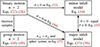Fig. 11.

Summary of all results: conditions to apply the infall models, their formulae, relations, and accuracy.

Applying the infall models and their small-angle approximation given by Eq. (46) to 344 isolated, relaxed halos of the Illustris-3 simulation in a mass range of m ∈ [1.4,16.4] × 10¹² M_⊙ and at distances from an observer in the range of d ∈ [18,162] Mpc, we found that the following assumptions made in Karachentsev & Kashibadze (2006), Karachentsev & Nasonova (2010), and Kim et al. (2020) do not hold: even for small separation angles θ < 10 deg of subhalos with respect to the centre of their parent halo, neither the velocity components perpendicular to the observers’ line of sight, nor the tangential velocity components vanish. Fig. 5 documents all the deviations from the true radial infall velocity and the expected vanishing velocity components. So we concluded that it is not sufficient to select galaxies at large distances from an observer to make perpendicular velocity components vanish, nor is it sufficient to select galaxies in front and behind their cluster centre along the observers’ line of sight to reduce the impact of the tangential velocity components. Moreover, as Fig. 6 revealed, it is not true that the true infall velocity always lies between the major and minor infall velocities. Overall, this only applied to 34% of all subhalos bound to the 344 halos and out to 1.5 times the zero-velocity radius into their Hubble flow region. In addition to that, we discovered that the possible motivation of the major infall model based on a vanishing total angular momentum of a cosmic structure is invalid as well. The total angular momenta of the halos in our selection are non-zero and their largest contribution originates from the angular momentum of the halo with respect to the observer. While the angular momentum within the halos is compatible with zero compared to the angular momentum of the entire structure with respect to the observer, as shown in Fig. 8 (right), the contributions of the angular momenta due to an offset between the centre of mass of the halo and the centre of mass of all its bound subhalos were non-negligible. Thus, even in the ideal case, when we knew the centre of mass and all masses of the subhalos, the additional constituents of the halo yielded a contribution to the angular momentum that may be relevant.

More positively, we also discovered that the velocity dispersions inferred from the infall models yield robust upper and lower bounds on the true velocity dispersion, as is depicted in Fig. 7. This allowed us to constrain the true velocity dispersion and all quantities that depend on it much more robustly than any quantities depending on the infall velocities directly. For the large halo distances to the observer considered in our selection d > 18 Mpc, the velocity dispersion based on the infall velocity in Eq. (46) even falls tightly onto the true velocity dispersion. So this may even be a good direct estimator instead of only upper and lower bounds for cosmic structures at large distances.

Applying the infall models to the M81 group also analysed in Karachentsev & Kashibadze (2006), we arrived at similar results for a newer dataset as is detailed in Müller et al. (2024). Yet, we could explain the large spread between the minor and major infall models as supported by a second selection of halos from the Illustris-3 simulation to imitate M81-like groups. For the latter simulations, we corroborated our results and thereby also showed that the infall models are purely based on kinematics and are thus independent of the masses involved in the models. Since the small-angle approximation also holds for the M81 group and 99% of all selected halos which are M81-group-like have θ < 10 deg, the results of our latter simulation are also similar in that respect. The main difference between the two selected halo sets is that the perpendicular velocity components as well as the intrinsic angular momentum of the structure increase in their importance at closer distances. From the observations of the M81 group, we arrived at the infall model approximations to the radial velocities as σ_r, min ≈ 96 km/s, σ_r, maj ≈ 564 km/s, σ_r, Δv ≈ 102 km/s. As the M81 group falls under the small angle approximation, the latter estimate is most likely to closest to the true radial velocity dispersion. A similar result is also obtained with the more elaborate Bayesian inference of the radial velocity dispersion from the infall model approximations (see Sect. 5.2), which, however, requires a larger amount of simulated M81-group-like halos in order to cover the feature space of all possible velocity dispersions in a more representative way.

One important aspect of observational data is the choice of reference frame. Corrections to account for the Earth’s motion around the sun are necessary, as they directly affect all lines of sight to all structures. The heliocentric velocities are measured to high precision, such that they are considered as observables seen from our cosmic position. Further corrections for the solar motion in the Milky Way, the Local-Group centroid or beyond up to the cosmic microwave background vary in their impact along different lines of sight and are subject to much larger uncertainties (see Aluri et al. 2023 for a recent overview of all relative motions and their tensions in our current concordance cosmology). Moreover, the infall models require fine-tuned assumptions about the velocity components to be accurate and transforming into one of these reference frames does not necessarily match these assumptions. While studies of bulk flows or inferences of cosmological parameters in the local universe are best performed in the fundamental rest frame of matter (see Ellis et al. 1985 and Maartens et al. 2024 for more details), they often rely on a sufficiently large local volume containing so many cosmic structures that the approximation of a pressureless dust density is valid. In contrast, our analysis of the M81 group is different, as we studied an individual cosmic structure. Thus, it is questionable whether any corrections for relative motions with respect to standard rest frames should be applied, as the transformations accumulate further uncertainties without making the infall models more accurate. For the corrections of the solar motion within the Local Group, we found that they are so small that they are likely to be absorbed in measurement uncertainties anyway.

In summary, the infall models cannot constrain the true radial infall velocity as originally expected due to the surprisingly large contributions of the perpendicular and tangential velocity components. However, the velocity dispersion calculated from the infall model velocities is a more robust quantity to constrain the true velocity dispersion and quantities depending on it. This is even true if the structure under analysis is not spherically symmetric, or is only sparsely sampled, as is shown by the simulated halos with only a few number of subhalos. Potentially, further summary-statistics based on a set of infall velocities could also be made robust bounds. One example is the Hubble flow fit to an ensemble of infall velocities.

How far the infall models can yield robust upper and lower bounds for binaries thus remains an open question. One possibility is to investigate if observations of tangential velocity components projected on the sky can alleviate the deviations or whether it is necessary to include satellite galaxies to the pair. An ideal system to study is the Local Group, for which respective observables are available (Benisty et al. 2022).

For galaxy clusters of masses above 10¹⁴ M_⊙ with velocity dispersions of 1000 km/s, the difference in the velocity dispersions of the major and minor infall models is assumed to be larger than for our halo selection with the true velocity dispersion being closer to the one of the minor infall model. Hence, in contrast to the original motivation for the major infall model, the minor infall model may yield more accurate velocity dispersions and dependent quantities than the major infall model for galaxy clusters. A further simulation of high-redshift clusters will also reveal if the velocity dispersion given by Eq. (46) actually yields the tightest constraint on the true velocity dispersion. If true, virial mass estimates of high-redshift clusters based on the difference of line-of-sight velocity components will be confirmed to be the most accurate estimate with the tightest confidence bounds. More generally, as corroborated by our study of the M81 group, any structure for which the small-angle approximation holds can employ this result. For all other structures, the major and minor infall models provide the most robust upper and lower limits to the radial velocity dispersion.

¹

https://www.tng-project.org/data/docs/scripts/

²

Amplitudes |⋅| can be negative, while the absolute (non-negative) size of a vector is denoted as ∥ ⋅ ∥₂.

³

As in Sect. 4, the fit excludes outliers with ||v_r, maj||₂ > 3000 km/s. Yet, only 1% (21) of all bound subhalos are affected by this cut.

Acknowledgments

We cordially thank the anonymous referee for suggesting valuable improvements, Rainer Weinberger, Dylan Nelson and Volker Springel for their further comments and discussion on the TNG simulations and Roy Maartens for his help on the rest-frame issue. DB is supported by a Minerva Fellowship of the Minerva Stiftung Gesellschaft für die Forschung mbH.

References

Aluri, P., Cea, P., Chingangbam, P., et al. 2023, Class. Quant. Grav., 40, 094001 [NASA ADS] [CrossRef] [Google Scholar]
Benisty, D., & Mota, D. 2025, A&A, 698, A43 [NASA ADS] [CrossRef] [EDP Sciences] [Google Scholar]
Benisty, D., Vasiliev, E., Evans, N. W., et al. 2022, ApJ, 928, L5 [NASA ADS] [CrossRef] [Google Scholar]
Benisty, D., Libeskind, N. I., & Hoffman, Y. 2025a, A&A, submitted [Google Scholar]
Benisty, D., Wagner, J., Haridasu, S., & Salucci, P. 2025b, ApJ, submitted [arXiv:2504.04135] [Google Scholar]
Chiboucas, K., Jacobs, B. A., Tully, R. B., & Karachentsev, I. D. 2013, AJ, 146, 126 [Google Scholar]
DESI Collaboration (Adame, A. G., et al.) 2024, AJ, 168, 58 [NASA ADS] [CrossRef] [Google Scholar]
Diaz, J. D., Koposov, S. E., Irwin, M., Belokurov, V., & Evans, N. W. 2014, MNRAS, 443, 1688 [CrossRef] [Google Scholar]
Ellis, G. F. R., Nel, S. D., Maartens, R., Stoeger, W. R., & Whitman, A. P. 1985, Phys. Rep., 124, 315 [Google Scholar]
Hawking, S. 1969, MNRAS, 142, 129 [Google Scholar]
Karachentsev, I. D., & Kashibadze, O. G. 2006, Astrophysics, 49, 3 [NASA ADS] [CrossRef] [Google Scholar]
Karachentsev, I. D., & Makarov, D. A. 1996, AJ, 111, 794 [NASA ADS] [CrossRef] [Google Scholar]
Karachentsev, I. D., & Nasonova, O. G. 2010, MNRAS, 405, 1075 [NASA ADS] [Google Scholar]
Karachentsev, I. D., Kashibadze, O. G., Makarov, D. I., & Tully, R. B. 2009, MNRAS, 393, 1265 [NASA ADS] [CrossRef] [Google Scholar]
Karachentsev, I. D., Makarov, D. I., & Kaisina, E. I. 2013, AJ, 145, 101 [Google Scholar]
Kim, Y. J., Kang, J., Lee, M. G., & Jang, I. S. 2020, ApJ, 905, 104 [NASA ADS] [CrossRef] [Google Scholar]
Maartens, R., Santiago, J., Clarkson, C., Kalbouneh, B., & Marinoni, C. 2024, JCAP, 2024, 070 [Google Scholar]
Müller, O., Heesters, N., Pawlowski, M. S., et al. 2024, A&A, 683, A250 [NASA ADS] [CrossRef] [EDP Sciences] [Google Scholar]
Nelson, D., Pillepich, A., Genel, S., et al. 2015, Astron. Comput., 13, 12 [Google Scholar]
Peirani, S., & de Freitas Pacheco, J. A. 2006, New Astron., 11, 325 [NASA ADS] [CrossRef] [Google Scholar]
Peñarrubia, J., Ma, Y.-Z., Walker, M. G., & McConnachie, A. 2014, MNRAS, 443, 2204 [Google Scholar]
Saadeh, D., Feeney, S. M., Pontzen, A., Peiris, H. V., & McEwen, J. D. 2016, Phys. Rev. Lett., 117, 131302 [NASA ADS] [CrossRef] [Google Scholar]
Said, K., Howlett, C., Davis, T., et al. 2025, MNRAS, 539, 3627 [Google Scholar]
Salomon, J. B., Ibata, R., Reylé, C., et al. 2021, MNRAS, 507, 2592 [NASA ADS] [Google Scholar]
Sohn, S. T., Anderson, J., & van der Marel, R. P. 2012, ApJ, 753, 7 [NASA ADS] [CrossRef] [Google Scholar]
Sorce, J. G., Gottlöber, S., Hoffman, Y., & Yepes, G. 2016, MNRAS, 460, 2015 [NASA ADS] [CrossRef] [Google Scholar]
Tully, R. B., Kourkchi, E., Courtois, H. M., et al. 2023, ApJ, 944, 94 [NASA ADS] [CrossRef] [Google Scholar]
Valade, A., Libeskind, N. I., Pomarède, D., et al. 2024, Nat. Astron., 8, 1610 [Google Scholar]
van der Marel, R. P., Fardal, M., Besla, G., et al. 2012, ApJ, 753, 8 [NASA ADS] [CrossRef] [Google Scholar]
van der Marel, R. P., Fardal, M. A., Sohn, S. T., et al. 2019, ApJ, 872, 24 [NASA ADS] [CrossRef] [Google Scholar]
Vogelsberger, M., Genel, S., Springel, V., et al. 2014, Nature, 509, 177 [Google Scholar]
Zjupa, J., & Springel, V. 2017, MNRAS, 466, 1625 [Google Scholar]

Appendix A: Observational data set

The data shown in Table A.1 is taken from Müller et al. (2024) except for the entries of M81 and M82 which are taken from Karachentsev et al. (2013). As stated in the latter, the measured heliocentric radial velocities are corrected for the motion of the sun within the Local-Group centroid frame as

$\begin{matrix} v_{LG} = v_{hel} & + 316 \frac{km}{s} (sin (b) sin (- 4^{°}) + cos (b) cos (- 4^{°}) cos (l - 93^{°})), \end{matrix}$ $\begin{aligned} v_\mathrm{LG} = v_\mathrm{hel}&+ 316~\tfrac{\mathrm{km}}{\mathrm{s}} \, \Big ( \sin (b) \sin (-4^\circ ) + \cos (b) \cos (-4^\circ ) \cos (l-93^\circ ) \Big ) \;, \end{aligned}$ (A.1)

in which b and l denote the coordinates of the galaxy in the Galactic coordinate system (following the IAU’s 1958 definition). The apex velocity of 316 km/s and the apex coordinates of (93° , − 4° ) in Galactic longitude and latitude are taken from Karachentsev & Makarov (1996). As stated in this work, uncertainties in the coordinates amount to 2 deg and to 5 km/s in the apex velocity. They need to be taken into account to obtain confidence bounds on v_LG. Consequently, uncertainties after applying the correction are larger than those in the heliocentric frame. No uncertainties are listed for v_LG in the data base of Karachentsev et al. (2013). As our proof-of-principle analysis focussed on accuracy and not precision, v_LG are listed without uncertainties, but the latter should be included in a full analysis of the data.

Table A.1.

M81 group members.

All Tables

Table A.1.

M81 group members.

In the text

All Figures

Fig. 1.

Three-dimensional motion of two galaxies and definition of notations. The maximum information a distant observer can measure is the velocity components along the line of sight v_l1, v_l2 to a high precision via spectroscopy, highly precise angle between the galaxy positions on the sky, θ, and line-of-sight distances r₁, r₂ with a precision depending on the probe used (see Tully et al. 2023 for recent examples).

In the text

	Fig. 2. Minor infall model: the line-of-sight velocity components of both galaxies are projected onto their connection line. The difference of these projections yields the relative radial velocity.
In the text

Fig. 3.

Major infall model for galaxy 1: the radial infall velocity of galaxy 1 onto galaxy 2 can be determined from the projection of the radial infall velocity and the line-of-sight velocity of galaxy 2 onto the line-of-sight of galaxy 1. An analogous procedure yields the major infall model for galaxy 2. Due to the asymmetry of this model, both radial infall velocities need not be of the same size.

In the text

	Fig. 4. Physical distances from an observer at the origin to the centre of mass of 344 isolated, relaxed halos versus their halo masses in the z = 0-snapshot of Illustris-3. In the notation of Sect. 3, \|r_halo\|≡\|r_cm\|.
In the text

Fig. 5.

Left: Reconstructed infall velocities by Eqs. (34), (37), and (46) for all subhalos (bound in dark colours, Hubble-flow subhalos in light colours) onto their parent-halo centre versus the true radial velocity by Eq. (22). Linear fits with 1-σ confidence bounds to the point clouds of the minor infall model and the velocity-difference approximation are shown in blue and grey, respectively. The fit for the major infall is not shown as its confidence bound covers the entire plot. Centre: Perpendicular velocities of all subhalos versus their distance to the observer (bound in black, Hubble-flow subhalos in grey). Only the six subhalos in the Hubble flow marked in blue have a tangential velocity close to zero. In the notation of Sect. 3, |r_subhalo|≡|r_j|. Right: Absolute value of the tangential velocity of all subhalos (bound in dark colours, Hubble-flow subhalos in light colours) versus their radial velocity. Only 337 subhalos with radial velocity close to zero also have a tangential velocity close to zero (marked in blue), while 3575 subhalos have a larger tangential velocity than radial one (marked in red).

In the text

Fig. 6.

Left: Radial velocity of all 5036 subhalos onto their parent halo versus the mass of their parent halo, highlighted in blue are those subhalos whose radial velocity lies between the minor and major infall velocity (dark colours mark bound halos, light colours mark subhalos in the Hubble flow). Centre: Same as the previous plot, but depending on the distance of the parent halo to the observer instead of the parent-halo mass. Right: Hubble-flow diagram for the most massive halo in our halo set to be compared with Fig. 7 of Kim et al. (2020). The major and minor infall velocities can be compared to the true radial infall velocity (dark colours mark bound halos, light colours mark subhalos in the Hubble flow), squared markers indicate which radial velocities lie between the minor and major infall velocities.

In the text

	Fig. 7. Velocity dispersions of bound subhalos for halos containing at least five bound subhalos j = 1, …, 109, calculated based on the minor and major infall models, as well as the infall velocity approximated by Eq. (46).
In the text

Fig. 8.

Left: Difference between the centre of mass of the parent halo and the centre of mass of the bound subhalos calculated as the mass-weighted sum of all their centre-of-mass positions versus the number of bound subhalos. The difference in the centre-of-mass positions is scaled to the zero-velocity radius of the halo for comparison. Centre: Total angular momentum as given by Eq. (49) versus the number of bound subhalos. Right: Individual components of the angular momentum given by Eqs. (50)–(54) with respect to the total one versus the number of bound subhalos.

In the text

Fig. 9.

Same as Fig. 5 but for the 281 M81-group-like halos. From all 5938 subhalos out to 1.5 r₀, 125 have a perpendicular velocity compatible with zero, 5427 have one that is larger than their line-of-sight velocity. For the bound subhalos, the numbers are 114 and 1925 out of 2099, respectively. 132 out of 5938 subhalos have a tangential velocity compatible with zero, for 5190, the tangential velocity exceeds the absolute value of the radial one. For the bound halos, the numbers are 118 and 1870, respectively.

In the text

Fig. 10.

Left: Infall-model velocities defined in Eqs. (34), (37), and (46) for each member of the M81 group (see Table A.1 for details on the data). Centre: Velocity dispersions of the infall models and the approximation of Eq. (46) of the bound subhalos in the simulation set up in Sect. 5.1 (same as Fig. 7) for j = 1, …, 281 halos. Dotted lines mark the velocity dispersions as determined for the M81 group members of Table A.1. Right: Ratios of absolute values of angular momenta as given by Eqs. (50)–(54) with respect to the total angular momentum (same as Fig. 8, right).

In the text

	Fig. 11. Summary of all results: conditions to apply the infall models, their formulae, relations, and accuracy.
In the text

Current usage metrics show cumulative count of Article Views (full-text article views including HTML views, PDF and ePub downloads, according to the available data) and Abstracts Views on Vision4Press platform.

Data correspond to usage on the plateform after 2015. The current usage metrics is available 48-96 hours after online publication and is updated daily on week days.

Initial download of the metrics may take a while.

[1] Aluri, P., Cea, P., Chingangbam, P., et al. 2023, Class. Quant. Grav., 40, 094001 [NASA ADS] [CrossRef] [Google Scholar]

[2] Benisty, D., & Mota, D. 2025, A&A, 698, A43 [NASA ADS] [CrossRef] [EDP Sciences] [Google Scholar]

[3] Benisty, D., Vasiliev, E., Evans, N. W., et al. 2022, ApJ, 928, L5 [NASA ADS] [CrossRef] [Google Scholar]

[4] Benisty, D., Libeskind, N. I., & Hoffman, Y. 2025a, A&A, submitted [Google Scholar]

[5] Benisty, D., Wagner, J., Haridasu, S., & Salucci, P. 2025b, ApJ, submitted [arXiv:2504.04135] [Google Scholar]

[6] Chiboucas, K., Jacobs, B. A., Tully, R. B., & Karachentsev, I. D. 2013, AJ, 146, 126 [Google Scholar]

[7] DESI Collaboration (Adame, A. G., et al.) 2024, AJ, 168, 58 [NASA ADS] [CrossRef] [Google Scholar]

[8] Diaz, J. D., Koposov, S. E., Irwin, M., Belokurov, V., & Evans, N. W. 2014, MNRAS, 443, 1688 [CrossRef] [Google Scholar]

[9] Ellis, G. F. R., Nel, S. D., Maartens, R., Stoeger, W. R., & Whitman, A. P. 1985, Phys. Rep., 124, 315 [Google Scholar]

[10] Hawking, S. 1969, MNRAS, 142, 129 [Google Scholar]

[11] Karachentsev, I. D., & Kashibadze, O. G. 2006, Astrophysics, 49, 3 [NASA ADS] [CrossRef] [Google Scholar]

[12] Karachentsev, I. D., & Makarov, D. A. 1996, AJ, 111, 794 [NASA ADS] [CrossRef] [Google Scholar]

[13] Karachentsev, I. D., & Nasonova, O. G. 2010, MNRAS, 405, 1075 [NASA ADS] [Google Scholar]

[14] Karachentsev, I. D., Kashibadze, O. G., Makarov, D. I., & Tully, R. B. 2009, MNRAS, 393, 1265 [NASA ADS] [CrossRef] [Google Scholar]

[15] Karachentsev, I. D., Makarov, D. I., & Kaisina, E. I. 2013, AJ, 145, 101 [Google Scholar]

[16] Kim, Y. J., Kang, J., Lee, M. G., & Jang, I. S. 2020, ApJ, 905, 104 [NASA ADS] [CrossRef] [Google Scholar]

[17] Maartens, R., Santiago, J., Clarkson, C., Kalbouneh, B., & Marinoni, C. 2024, JCAP, 2024, 070 [Google Scholar]

[18] Müller, O., Heesters, N., Pawlowski, M. S., et al. 2024, A&A, 683, A250 [NASA ADS] [CrossRef] [EDP Sciences] [Google Scholar]

[19] Nelson, D., Pillepich, A., Genel, S., et al. 2015, Astron. Comput., 13, 12 [Google Scholar]

[20] Peirani, S., & de Freitas Pacheco, J. A. 2006, New Astron., 11, 325 [NASA ADS] [CrossRef] [Google Scholar]

[21] Peñarrubia, J., Ma, Y.-Z., Walker, M. G., & McConnachie, A. 2014, MNRAS, 443, 2204 [Google Scholar]

[22] Saadeh, D., Feeney, S. M., Pontzen, A., Peiris, H. V., & McEwen, J. D. 2016, Phys. Rev. Lett., 117, 131302 [NASA ADS] [CrossRef] [Google Scholar]

[23] Said, K., Howlett, C., Davis, T., et al. 2025, MNRAS, 539, 3627 [Google Scholar]

[24] Salomon, J. B., Ibata, R., Reylé, C., et al. 2021, MNRAS, 507, 2592 [NASA ADS] [Google Scholar]

[25] Sohn, S. T., Anderson, J., & van der Marel, R. P. 2012, ApJ, 753, 7 [NASA ADS] [CrossRef] [Google Scholar]

[26] Sorce, J. G., Gottlöber, S., Hoffman, Y., & Yepes, G. 2016, MNRAS, 460, 2015 [NASA ADS] [CrossRef] [Google Scholar]

[27] Tully, R. B., Kourkchi, E., Courtois, H. M., et al. 2023, ApJ, 944, 94 [NASA ADS] [CrossRef] [Google Scholar]

[28] Valade, A., Libeskind, N. I., Pomarède, D., et al. 2024, Nat. Astron., 8, 1610 [Google Scholar]

[29] van der Marel, R. P., Fardal, M., Besla, G., et al. 2012, ApJ, 753, 8 [NASA ADS] [CrossRef] [Google Scholar]

[30] van der Marel, R. P., Fardal, M. A., Sohn, S. T., et al. 2019, ApJ, 872, 24 [NASA ADS] [CrossRef] [Google Scholar]

[31] Vogelsberger, M., Genel, S., Springel, V., et al. 2014, Nature, 509, 177 [Google Scholar]

[32] Zjupa, J., & Springel, V. 2017, MNRAS, 466, 1625 [Google Scholar]