| Issue |
A&A
Volume 697, May 2025
|
|
|---|---|---|
| Article Number | L9 | |
| Number of page(s) | 7 | |
| Section | Letters to the Editor | |
| DOI | https://doi.org/10.1051/0004-6361/202553735 | |
| Published online | 16 May 2025 | |
Letter to the Editor
On the limitations of using metric radio bursts as diagnostic tools for interplanetary coronal mass ejections
1
Department of Physics, Ahmednagar College, Station Road, Ahilyanagar, 414001 Maharashtra, India
2
Udaipur Solar Observatory, Physical Research Laboratory, Dewali, Badi Road, Udaipur, 313 001 Rajasthan, India
⋆ Corresponding author: This email address is being protected from spambots. You need JavaScript enabled to view it.
Received:
13
January
2025
Accepted:
15
April
2025
Abstract
Aims. Metric radio bursts are often said to be valuable diagnostic tools for studying the near-sun kinematics and energetics of the interplanetary coronal mass ejections (ICMEs). Radio observations also serve as indirect tools to estimate the coronal magnetic fields. However, how these estimated coronal magnetic fields are related to the magnetic field strength in the ICME at 1 AU has rarely been explored. Our aim was to establish a relation between the coronal magnetic fields obtained from the radio observations very close to the Sun and the magnetic field measured at 1 AU when the ICME arrives at the Earth.
Methods. We performed statistical analyses of all metric type II radio bursts in solar cycles 23 and 24 that were found to be associated with ICMEs. We estimated the coronal magnetic field associated with the corresponding CME near the Sun (middle corona) using a split-band radio technique and compared them with the magnetic fields recorded at 1 AU with in situ observations.
Results. We found that the estimated magnetic fields near the Sun using radio techniques are not well correlated with the magnetic fields measured at 1 AU using in situ observations. This could be due to the complex evolution of the magnetic field as it propagates through the heliosphere.
Conclusions. Our results suggest that while metric radio observations can serve as effective proxies for estimating magnetic fields near the Sun, they may not be as effective close to the Earth. At least, no linear relation could be established using metric radio emissions to estimate the magnetic fields at 1 AU with acceptable error margins.
Key words: Sun: activity / Sun: corona / Sun: coronal mass ejections (CMEs) / Sun: heliosphere / Sun: magnetic fields / Sun: radio radiation
© The Authors 2025
 Open Access article, published by EDP Sciences, under the terms of the Creative Commons Attribution License (https://creativecommons.org/licenses/by/4.0), which permits unrestricted use, distribution, and reproduction in any medium, provided the original work is properly cited.
This article is published in open access under the Subscribe to Open model. This email address is being protected from spambots. You need JavaScript enabled to view it. to support open access publication.
1. Introduction
The coronal magnetic field (B) serves as a fundamental factor governing the formation, evolution, and dynamics of solar corona structures (Dulk & McLean 1978). Measuring these fields directly from observations, particularly in the chromosphere and corona, remains a significant challenge in solar physics (White 2002; Carley et al. 2020, and the references therein). Various methods exist to infer coronal magnetic fields, encompassing techniques such as coronal seismology (Jess et al. 2016), Zeeman splitting of spectral lines (Lin et al. 2004), and extrapolation methods (Wiegelmann et al. 2017), though constrained to specific regions of the solar atmosphere. Among these, including the shock-standoff technique (Gopalswamy & Yashiro 2011) and radio techniques, estimations from solar radio bursts offer valuable insights into the coronal magnetic field, especially in the middle corona (Carley et al. 2017).
Solar eruptive phenomena, such as solar flares and coronal mass ejections (CMEs), significantly influence space weather dynamics. These events often trigger energetic electron acceleration, generating radio emissions like type II and type IV bursts observed in the metric and decameter-hectometric (DH) frequency range (Dulk & Suzuki 1980). Taking advantage of these radio bursts enables the study of the CME early evolution and dynamics near the Sun (within 10 solar radii), which can help in estimating CME magnetic fields and in assessing their geo-effectiveness. Since radio observations consist of solar, heliospheric, and ionospheric space weather phenomena, radio techniques can offer a practical approach to probing the solar atmosphere’s magnetic field (White 2004; Gopalswamy 2006). Combining diverse radio techniques with broadband spectroscopic solar radio imaging allows coronal magnetic fields to be derived in various solar regions (Ramesh & Sastry 2000; Kumari et al. 2017a). However, while metric type II radio bursts and their spectral characteristics, such as split-band features, have long served as robust tools for direct coronal magnetic field estimation (Smerd & Sheridan 1974; Vršnak & Cliver 2008; Mahrous et al. 2018), their correlation with magnetic fields observed at 1 AU during near-Earth interplanetary coronal mass ejections (ICMEs) remains less explored.
Previously, researchers have investigated metric and DH radio bursts and their correlation with electron accelerations, coronal mass ejections (CMEs), and their variations throughout the solar cycle (Kahler et al. 2019; Kumari et al. 2023). However, to the best of our knowledge, no prior study has explored how the characteristics of metric radio bursts can provide insights into space weather phenomena, such as ICMEs. For this study we investigated the long-term datasets of solar radio bursts and ICMEs over solar cycles 23 and 24 to explore the feasibility of using radio techniques for coronal magnetic field estimation and their relationship with in situ magnetic field observations at 1 AU during ICME events.
This article is structured as follows. Section 2 discusses the observational data utilized in this study along with detailed data analysis procedures. The findings of the present study are presented in Section 3. Section 4 contains a discussion of the results and their implications, followed by a summary of the study.
2. Observations and data analysis
For this study, we identified 88 metric type IIs associated with the ICMEs of solar cycles 23 and 24 (1997–2019). The CME event list used here was obtained from the Coordinated Data Analysis Workshop (CDAW; Yashiro et al. 2004) database1, which is a manual catalogue of the CMEs and their properties recorded by the Solar and Heliospheric Observatory’s (SOHO) Large Angle and Spectrometric Coronagraph (LASCO) white-light coronagraph observations (Brueckner et al. 1995). This list has the CME properties and parameters such as linear and second-order speed, kinetic energy, mass, angle of position. Additionally, we used the ICME list2 provided by Richardson & Cane (2010), which contains the dates and times of plasma disturbances of the ICMEs, duration, magnetic field strength, and speed, among other details, and associated with the date and time of the CMEs when they reach 1 AU. This list consists of ICME events since January 1996. Following the CME events associated with the ICME events, the radio data obtained from the Solar Electro-Optical Network (SEON) database3 was used for the data analysis. It consists of two networks: (1) the Solar Observing Optical Network (SOON) and (2) the Radio Spectral Telescope Network (RSTN). The RSTN contains four solar radio observatories across the globe. The radio database from the Radio Spectral Telescope Network (RSTN) was utilized; this data consists of the Solar Radio Spectrographs (SRS) over a wide band (25–180 MHz), where the Radio Interference Measuring Set (RIMS) is the instrument detecting radio emissions at eight different frequencies. For the missing type IIs in the SEON RSTN database, eCallisto data4 was referred. Furthermore, Hiraiso Radio Spectrograph (HiRAS) data (Kondo et al. 1995) managed by the National Institute of Information and Communications Technology (NICT5) was also utilized to obtain the spectra of type II bursts. We used the OMNI 5 min data from NASA/GSFC’s OMNIweb for the related ICMEs. The data was accessed through NASA’s Coordinated Data Analysis Web (CDAWeb6). We utilized the 5 min high-resolution flow speed (km/s) and the magnetic field (nT) data.
Out of the 88 events identified, only 31 metric type IIs for solar cycles 23 (1996–2008) and 24 (2008–2019) had split-band features identified in the solar dynamic spectra. Few of the type IIs had a start frequency > 180 MHz (Appendix A.1). The 31 CME-ICME associated split-band events comprised a fundamental band and a harmonic band. As shown in Figure 1, these events also exhibited a clear three-part structure (core, cavity and leading edge, Riley et al. 2008). For radio data analysis, the dynamic spectra were cleaned and the radio frequency interference was removed. We used the four-fold Newkirk density model (Newkirk 1961) to convert the type II frequencies into radio heights. We used the following equation to estimate the magnetic field strength of 31 split-bands (CME-ICME associated events) (Smerd & Sheridan 1974; Vršnak et al. 2002)
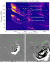 |
Fig. 1. Upper panel: Dynamic spectrum of type II burst recorded by Learmonth Observatory on 6 July 2006 in the range 180–25 MHz. The type II burst started at 08:24 UTC and lasted for 17 minutes. The white dotted lines represent the fundamental and harmonic bands. Lower panel: Three-part structure of the CME with a core, cavity, and leading edge recorded by LASCO C2 on 6 July 2006 at 09:06 UTC and 10:06 UTC. The CME started at 08:54 UTC (Appendix A.1). |
![Mathematical equation: $$ \begin{aligned} B = 5.1 \times 10^{-5} \times F_{\rm LB}\times v_{\rm A},~~[\mathrm{G}] \end{aligned} $$](/articles/aa/full_html/2025/05/aa53735-25/aa53735-25-eq1.gif) (1)
(1)
where B is the magnetic field strength derived from the type II bursts in gauss, FLB (MHz) is the lower band frequency of the undisturbed corona (Vršnak et al. 2002), and vA (km/s) is the Alfvén speed. The magnetic fields obtained were compared with the magnetic fields recorded at 1 AU. A master list of solar cycle 23 and 24 events was created and divided into two tables. Table A.1 is for type IIs and CME events, and lists date, start time (UT), end time (UT), duration (min), start and end frequency (MHz), start time of CME (UT), CME’s width (deg), and CME speed (km/s) obtained from the CDAW database. Table A.2 is for ICME events, and lists date, start time (UT), start and end time of the disturbances in plasma along with its start-end date, ICME Plasma speed (km/s), magnetic field strength (G) obtained from the Richardson–Cane catalogue and the shock speed and the B field strength (G), which obtained from the radio data analysis of type II burst as described in this section.
3. Results
3.1. Case study
The dynamic spectra of the slowly drifting type II burst with a fundamental and harmonic band, which occurred on 6 July 2006 at 08:23:12 UT, is displayed in Fig. 1. The CME with a distinct three-part structure begins at 08:54 UT in the lower panel and is subsequently displayed, followed by a disturbance recorded near Earth at 21:36 UT on 9 July 2006 (Richardson & Cane 2010) (Appendix A.2), where the ICME started on 10 July 2006 at 21:00 UT and ended on 11 July 2006 at 19:00 UT, lasting for 22 hours (see Fig. 2). The CME propagated at a speed of 911 km/s, which was higher than the shock speed estimated from the type II radio burst (≈369 km/s). The associated speed from the Richardson catalogue was 380 km/s. The difference in speeds of type II, CME, and ICME arises because the CME’s interaction with the surroundings affects their speed (Gopalswamy et al. 2000); in this case, we have a CME with a speed of ≈1100 km/s (Kumari et al. 2023). The split-band type IIs bursts are seen as well-accepted techniques to estimate magnetic field strengths just above the shock (i.e. B in gauss derived from the type II radio bursts) (Smerd et al. 1975; Vršnak et al. 2002; Cho et al. 2007; Kumari et al. 2017b). Based on this and as described in Sect. 2, we obtained three values for electron density (cm−1), three values for each FLB (MHz) and FUB (MHz), three values for heliocentric distance (R⊙) for each corresponding value (i.e. six values of heliocentric distance, R⊙), and estimated three values of the magnetic field strength (B (G)). These values served as a basis for our power-law fit equation (Kumari et al. 2019)
![Mathematical equation: $$ \begin{aligned} B = 2 \times r^{-a}~~[\mathrm{G}], \end{aligned} $$](/articles/aa/full_html/2025/05/aa53735-25/aa53735-25-eq2.gif) (2)
(2)
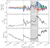 |
Fig. 2. Associated plot of ICME parameters obtained from Omni data for the type II burst and CME that occurred on 6 July 2006. The top panel illustrates the Bx, By, and Bz vector components of the B field (G); the middle panel shows the average strength of the B field vector (G); and the bottom panel shows the flow speed across the timeline of the event. The vertical dotted line shows the near-Earth shock arrival at 21:36 UT on 9 July 2006 and the grey-shaded region shows the start and end time of the disturbance in the plasma (Richardson & Cane 2010), starting at 19:00 UT on 9 July 2006 and ending at 21:00 UT on 11 July 2006. |
where B is the average magnetic field and r is the heliocentric distance (in terms of R⊙, which is the radius of the photospheric Sun). At the range of 1.36–1.5 R⊙ and the lower band frequency range of FLB ≈ 141 − 101 MHz, we estimated the average B field strength of 0.45 G using the Equation (2), for the type II burst that occurred on 6 July 2006. The mean B (G) field associated with the upstream field just before the ICME (B1 AU (G)) was found to be 4.5 × 10⁻⁵ (G). This associated ICME lasted 22 hours (10 July 2006 21:00 UT to 11 July 2006 19:00 UT). The B1 AU (G) was significantly attenuated compared to the estimated coronal B field strength (G), as expected due to the propagation of the CME in the heliosphere and its interaction with other magnetic structures there. Since the magnetic field derived from radio observations were from the lower frequency bands, which can be associated with the undisturbed corona, and the ICME field is, by definition, the disturbed field, we used the B fields from the upstream field (pre-shock region). For this study we also explored the ICME parameters obtained from OMNIweb7 (NASA/GSFC). The average strength of the B field vector (G) was obtained to be 9.4 × 10⁻⁵ (G) (mean) with the mean flow speed of 369 km/s for the start and end date time of the ICME disturbance (see Figure 2). These values are consistent with those of the values in the Richardson–Cane catalogue.
3.2. Statistical study of split-band type II bursts
Similarly, we derived the B field strength values (BRadio (G)) for 31 such split-band observations for the solar cycles of 23 and 24, varying from 0.04 G to 4.59 G for the heliocentric distance (r) ranging from 1.1 R⊙ to 2.5 R⊙. We note that the ‘a’ in the Equation (2) varies for individual split-band observations. We calculated the upstream magnetic field values, B1 AU (G) at 1 AU in the range 4.5 − 20.8 × 10⁻⁵ G obtained from the OMNI database. A correlation between the near-Sun coronal magnetic fields and near-Earth upstream magnetic field strength observed just before the ICME was established by linearly fitting the magnetic fields (B1 AU (G)) at 1 AU and the estimated (BRadio (G)) was derived from the type II radio bursts (see Fig. 3), yielding a slope of 0.36 and an intercept of 8.19, suggesting a linearly weak relation. The weak correlation was confirmed by the obtained correlation coefficient (r of 0.14; see Fig. 3).
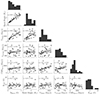 |
Fig. 3. Correlation between various parameters of 31 CME- and ICME-related events. The scattered hexagonal points are the data that contain shock height (R⊙), Fstart (MHz), Fend (MHz), speed of radio bursts (km/s), ICME speed (km/s), CME speed (km/s), and magnetic field strength derived from type IIs and obtained with ICME in situ measurements. |
We used a four-fold Newkirk density model to estimate the shock heights (the radial distance from the Sun’s centre to the leading edge of the shock wave that forms ahead of a CME as it propagates through the solar corona), in terms of R⊙, close to the corona. We used three-fold and five-fold Newkirk density models to estimate the error bars for these shock height values (see Fig. 3). These height estimate errors were then used to set the upper and lower limits of the error bars in the shock speed calculations. Similarly, we averaged over ≈ 15 min of upstream magnetic field values at 1 AU and used the rms values to estimate the uncertainties in B1 AU (G) values in the pre-shock region (see Fig. 3). The uncertainties in the speed of CME (VCME) were estimated assuming linear propagation of the CME leading edge. The resulting uncertainties in the present study and correlation coefficients with error bars are shown in Fig. 3.
4. Summary and discussion
Figure 3 shows that the magnetic fields near the Sun estimated using radio techniques are not well correlated with the magnetic field measured at 1 AU using in situ observations. Previous studies have suggested that metric radio observations can serve as effective proxies for estimating magnetic fields near the Sun (Vršnak & Cliver 2008; Kumari et al. 2017a, and the reference therein). However, to the best of our knowledge, there are no event specific or comprehensive long-term studies using solar radio bursts to estimate the heliospheric magnetic fields. Our findings in this study (see Fig. 3 and Table A.2) strongly indicate that no linear relation could be established using metric radio emissions to estimate the magnetic fields at 1 AU with acceptable error margins. This suggests that metric radio observations cannot serve as effective proxies for estimating magnetic fields close to the Earth. This could be due to the complex evolution of the magnetic field structures as it propagates through the heliosphere (see for a review, Owens & Forsyth 2013). It is well known that CMEs are subject to rotation, deflection, and interaction (with solar wind and/or CME-CME interaction) (Palmerio et al. 2021; Sioulas et al. 2023, and the reference therein). However, we have not accounted for these conditions in our study due to the non-availability of radio data points between ≈2 R⊙ and 1 AU, which are to be investigated in further studies with the availability of Parker Solar Probe (PSP) and Solar Orbiter (SolO) data. The CME-ICME speed is correlated, suggesting that other factors such as speed can help understand the predictive patterns.
This study and the findings of this article can be summarized as follows:
-
Estimated B fields in the middle corona using split-band: We used the split-band observations to estimate magnetic fields within the middle corona. The split-band technique is an indirect measurement of magnetic field strengths just above the CME-driven shock, performed by analyzing different frequency bands of type II radio bursts.
-
Statistical analysis of radio bursts associated with ICMEs: Through statistical analysis, we investigated radio bursts associated with ICMEs. We also examined the start and end frequencies, bandwidths, and duration of radio emissions observed during ICME events. We aimed to identify a relation indicative of magnetic field variations and associated CMEs and ICMEs.
-
Relation between the magnetic field near the Sun and at 1 AU: Our results show almost no clear linear relation between the magnetic field strength near the Sun obtained with metric radio observations and in situ measurements of the magnetic field associated with upstream and/or shock transition fields just before the ICME. Hence, we could not establish any empirical relation that provides a means to estimate the magnetic field intensity when the disturbance reaches the Earth, based on measurements obtained closer to the Sun. This indicates that metric radio observations have become less reliable for estimating magnetic fields closer to Earth.
Acknowledgments
AK acknowledges the ANRF Prime Minister Early Career Research Grant (PM ECRG) program. The authors acknowledge the Param Vikram-1000 High Performance Computing Cluster of the Physical Research Laboratory (PRL). All the authors acknowledge the event lists provided by the Space Weather Prediction Center and the ICME catalogue compiled by Ian Richardson and Hilary Cane. The authors acknowledge the sunpy package, the Coordinated Data Analysis Workshop (CDAW) catalogue, Solar Electro-Optical Network’s (SEON) Radio Spectral Telescope Network (RSTN) data, eCallisto data, National Institute of Information and Communications Technology’s (NICT) Hiraiso Radio Spectrograph (HiRAS) data, Solar and Heliospheric Observatory’s (SOHO) Large Angle and Spectrometric Coronagraph (LASCO), and NASA/GSFC’s OMNIweb database.
References
- Brueckner, G. E., Howard, R. A., Koomen, M. J., et al. 1995, Sol. Phys., 162, 357 [NASA ADS] [CrossRef] [Google Scholar]
- Carley, E. P., Vilmer, N., Simões, P. J. A., & Ó Fearraigh, B. 2017, A&A, 608, A137 [NASA ADS] [CrossRef] [EDP Sciences] [Google Scholar]
- Carley, E. P., Vilmer, N., & Vourlidas, A. 2020, Front. Astron. Space Sci., 7, 79 [Google Scholar]
- Cho, K.-S., Lee, J., Gary, D. E., Moon, Y.-J., & Park, Y. D. 2007, ApJ, 665, 799 [NASA ADS] [CrossRef] [Google Scholar]
- Dulk, G. A., & McLean, D. J. 1978, Sol. Phys., 57, 279 [CrossRef] [Google Scholar]
- Dulk, G. A., & Suzuki, S. 1980, A&A, 88, 203 [NASA ADS] [Google Scholar]
- Gopalswamy, N. 2006, Washington DC American Geophysical Union Geophysical Monograph Series, 165, 207 [NASA ADS] [Google Scholar]
- Gopalswamy, N., & Yashiro, S. 2011, ApJ, 736, L17 [NASA ADS] [CrossRef] [Google Scholar]
- Gopalswamy, N., Lara, A., Lepping, R. P., et al. 2000, Geophys. Res. Lett., 27, 145 [NASA ADS] [CrossRef] [Google Scholar]
- Jess, D. B., Reznikova, V. E., Ryans, R. S. I., et al. 2016, Nat. Phys., 12, 179 [NASA ADS] [CrossRef] [Google Scholar]
- Kahler, S. W., Ling, A. G., & Gopalswamy, N. 2019, Sol. Phys., 294, 134 [Google Scholar]
- Kondo, T., Isobe, T., Igi, S., Watari, S., & Tokumaru, M. 1995, J. Commun. Res. Lab., 42, 111 [Google Scholar]
- Kumari, A., Ramesh, R., Kathiravan, C., & Wang, T. J. 2017a, Sol. Phys., 292, 161 [NASA ADS] [CrossRef] [Google Scholar]
- Kumari, A., Ramesh, R., Kathiravan, C., & Wang, T. J. 2017b, Sol. Phys., 292, 177 [NASA ADS] [CrossRef] [Google Scholar]
- Kumari, A., Ramesh, R., Kathiravan, C., Wang, T. J., & Gopalswamy, N. 2019, ApJ, 881, 24 [NASA ADS] [CrossRef] [Google Scholar]
- Kumari, A., Morosan, D. E., Kilpua, E. K. J., & Daei, F. 2023, A&A, 675, A102 [NASA ADS] [CrossRef] [EDP Sciences] [Google Scholar]
- Lin, H., Kuhn, J. R., & Coulter, R. 2004, ApJ, 613, L177 [Google Scholar]
- Mahrous, A., Alielden, K., Vršnak, B., & Youssef, M. 2018, JASTP, 172, 75 [Google Scholar]
- Newkirk, G., Jr. 1961, ApJ, 133, 983 [NASA ADS] [CrossRef] [Google Scholar]
- Owens, M. J., & Forsyth, R. J. 2013, Liv. Rev. Sol. Phys., 10, 5 [Google Scholar]
- Palmerio, E., Nieves-Chinchilla, T., Kilpua, E. K. J., et al. 2021, J. Geophys. Res. Space Phys., 126, e2021JA029770 [NASA ADS] [CrossRef] [Google Scholar]
- Ramesh, R., & Sastry, C. V. 2000, A&A, 358, 749 [Google Scholar]
- Richardson, I. G., & Cane, H. V. 2010, Sol. Phys., 264, 189 [NASA ADS] [CrossRef] [Google Scholar]
- Riley, P., Lionello, R., Mikić, Z., & Linker, J. 2008, ApJ, 672, 1221 [NASA ADS] [CrossRef] [Google Scholar]
- Sioulas, N., Huang, Z., Shi, C., et al. 2023, ApJ, 943, L8 [CrossRef] [Google Scholar]
- Smerd, S. F., & Sheridan, K. V. 1974, in Coronal Disturbances, ed. G. A. Newkirk, Proc. IAU Symp., 57, 389 [NASA ADS] [CrossRef] [Google Scholar]
- Smerd, S. F., Sheridan, K. V., & Stewart, R. T. 1975, Astrophys. Lett., 16, 23 [NASA ADS] [Google Scholar]
- Vršnak, B., & Cliver, E. W. 2008, Sol. Phys., 253, 215 [Google Scholar]
- Vršnak, B., Magdalenić, J., Aurass, H., & Mann, G. 2002, A&A, 396, 673 [NASA ADS] [CrossRef] [EDP Sciences] [Google Scholar]
- White, S. M. 2002, in American Astronomical Society Meeting Abstracts, 200, 49.03 [Google Scholar]
- White, S. M. 2004, Astrophysics and Space Science Library, 314, 89 [Google Scholar]
- Wiegelmann, T., Petrie, G. J. D., & Riley, P. 2017, Space Sci. Rev., 210, 249 [CrossRef] [Google Scholar]
- Yashiro, S., Gopalswamy, N., Michalek, G., et al. 2004, J. Geophys. Res. Space Phys., 109, A07105 [NASA ADS] [CrossRef] [Google Scholar]
Appendix A: Tables containing detailed information about the events studied.
Various parameters of type II bursts and CMEs associated with the ICMEs in Table A.2
Various ICME parameters associated with the type II bursts and CMEs in Table A.1
All Tables
Various parameters of type II bursts and CMEs associated with the ICMEs in Table A.2
Various ICME parameters associated with the type II bursts and CMEs in Table A.1
All Figures
|
Fig. 1. Upper panel: Dynamic spectrum of type II burst recorded by Learmonth Observatory on 6 July 2006 in the range 180–25 MHz. The type II burst started at 08:24 UTC and lasted for 17 minutes. The white dotted lines represent the fundamental and harmonic bands. Lower panel: Three-part structure of the CME with a core, cavity, and leading edge recorded by LASCO C2 on 6 July 2006 at 09:06 UTC and 10:06 UTC. The CME started at 08:54 UTC (Appendix A.1). |
| In the text | |
|
Fig. 2. Associated plot of ICME parameters obtained from Omni data for the type II burst and CME that occurred on 6 July 2006. The top panel illustrates the Bx, By, and Bz vector components of the B field (G); the middle panel shows the average strength of the B field vector (G); and the bottom panel shows the flow speed across the timeline of the event. The vertical dotted line shows the near-Earth shock arrival at 21:36 UT on 9 July 2006 and the grey-shaded region shows the start and end time of the disturbance in the plasma (Richardson & Cane 2010), starting at 19:00 UT on 9 July 2006 and ending at 21:00 UT on 11 July 2006. |
| In the text | |
|
Fig. 3. Correlation between various parameters of 31 CME- and ICME-related events. The scattered hexagonal points are the data that contain shock height (R⊙), Fstart (MHz), Fend (MHz), speed of radio bursts (km/s), ICME speed (km/s), CME speed (km/s), and magnetic field strength derived from type IIs and obtained with ICME in situ measurements. |
| In the text | |
Current usage metrics show cumulative count of Article Views (full-text article views including HTML views, PDF and ePub downloads, according to the available data) and Abstracts Views on Vision4Press platform.
Data correspond to usage on the plateform after 2015. The current usage metrics is available 48-96 hours after online publication and is updated daily on week days.
Initial download of the metrics may take a while.