© The Authors 2025

1. Introduction

Theoretical research on the formation of stars and their accretion discs is far from determining a firm conclusion on nature of these processes. Even if we were to restrict the investigation to the formation of a single star from a molecular gas cloud, the field is still widely open, since the various clouds differ from one another in many parameters (form, mass, motion, strength of magnetic field, etc) and their collapse can be triggered by several effects (mass accretion and/or slow compression leading to the infringement of the stability limit, a shock wave created by a supernova explosion, etc). During the collapse, the physical interactions playing an essential role vary in space and time. The description of the collapse is therefore a challenging task.

The elaboration of the ‘inside-out’ collapse model of isothermal gas clouds had begun with Shu (1977). The present-day version of the model reckons with several different phases of the collapse. (For a brief summary on the topic, see, e.g. Basu 2015) The first one is a ‘free fall’ phase, which is essentially isothermal (the cloud remains optically thin and its cooling is provided by the radiation of molecular hydrogen and dust particles). This phase ends with the formation of an optically thick ‘first core’ in the cloud’s centre. Further mass accretion leads to the heating of the core. When the temperature has reached close to 2000 K, a massive dissociation of hydrogen molecules begins and the core starts to collapse again. The second collapse is halted by the ionisation of hydrogen atoms and the formation of the protostar, which continues to accrete material from the surrounding disc.

The cloud core collapse has also been modeled as a successive infall of thin spherical shells onto the disc, which is where each gas parcel is accreted at a radius where its specific angular momentum matches the local Keplerian one (see, e.g. Hueso & Guillot 2005; Takahashi et al. 2013). In the work of Hueso & Guillot (2005), the outer part of the disc is fed by the infalling material from the remnant of the collapsing molecular cloud and the governing equation of the evolution of the (axisymmetric) disc (Lynden-Bell & Pringle 1974) is augmented by a source term responsible for the infalling material.

In the model described in the work of Takahashi et al. (2013), the redistribution of the angular momentum of each thin spherical shell begins right after it is accreted onto the disc due to the gravitational torques that are awakened for the Toomre parameter (Toomre 1964) falling in the interval Q < 2 by using an effective α viscosity parametrised by Q. The effect of the disc’s radial pressure gradient on its rotation and mass distribution is neglected in their model; however, according to our present study, these properties could be important.

Studying the time evolution of the collapse of a molecular cloud, when a proto-disc has already formed around the protostar might be relevant, since under some specific circumstances, planetesimal formation can already begin when the protoplanetary disc has not yet formed entirely (Drążkowska & Dullemond 2018). In this phase, the outer part of the disc is fed by the infalling material from the remnant of the collapsing molecular cloud.

For the formation of star-planet systems, the most important processes take place in the inner, densest region of the collapsing cloud. As we can see, its evolution is a highly complicated process. Those less dense parts of the cloud that are further away from the rotation axis will eventually form the outer part of the disc. From the viewpoint of the formation of the star-planet system, the main role of this outer part is to gradually absorb the excess angular momentum from the disc’s inner part, thus making accretion possible by promoting the outward transport of angular momentum. Since it also contains solid material, the outer disc might be able to supply material for planet formation for a long enough time interval in the form of inward-directed pebble flux, being necessary for the formation of larger planetesimals by the streaming instability (Youdin & Goodman 2005) and their further growth to planetary cores and protoplanets mainly via pebble accretion (Lambrechts & Johansen 2012). To estimate the inward transport of the solid particles, we have to know the structure of the disc’s outer part, where the gas dynamics may significantly deviate from Keplerian rotation due to a steep radial pressure gradient. Our aim is therefore to describe the state of the disc far from the centre, right after it has formed; namely, in the epoch where the disc is already sufficiently ‘flat’ to allow for the use of a two-dimensional model, but the gas parcels still have the same angular momentum as prior to the collapse of the molecular cloud.

In this work, we derive the structure and motion of the disc’s outer part from the state of the progenitor molecular cloud it has formed from. The latter is described as an isothermal gas sphere; namely, a Bonnor–Ebert (BE) sphere (see Bonnor 1956 and Ebert 1955). Despite its simplicity, this model can also be a good approximation of real cases (cf. Alves et al. 2001). We assume that initially the BE sphere rotates as a rigid body, being slightly supercritical.

The most important result of our work is that for rapidly rotating cloud cores, the pressure gradient may play a significant role in shaping the structure of the outer disc. To highlight the importance of the role played by the radial pressure gradient within the forming disc, we compare our results with those found on the basis of the model from Takahashi et al. (2013).

2. Description of the physical model

We assumed a non-magnetised interstellar gas cloud with a homogeneous chemical composition and zero temperature gradient, which is slowly rotating as a solid body. The slow rotation implies that the cloud’s mass distribution is essentially spherically symmetric, namely, it is a Bonnor–Ebert sphere. However, if the ratio of central density to density on the edge surpasses a critical value of about 14.1, the system is unstable, and a small perturbation will lead to its gravitational collapse. This may eventually lead to the formation of a central protostar and a thin accretion disc around it.

We aim to model the final state of the collapsing BE sphere without following the dynamics of the collapse. This can be achieved by first making some assumptions. First, we suppose that the cloud retains its axial symmetry throughout the collapse. We also suppose that the temperature remains constant during the collapse. This assumption will surely not hold for the central, denser parts of the collapsing cloud, but can be accepted for the parts farther away from the axis of rotation, which will eventually form the outer part of the disc. As a further assumption, we neglected the transport of angular momentum during the collapse, at least for the above-mentioned outer parts of the cloud. Finally, we also neglected the mass loss of the cloud, which could occur if the inner part were to lose its angular momentum by emitting bipolar jets. These basic assumptions enabled us to set up equations, which connect the structure of the final state to that of the initial state just prior to collapse. The solution of these equations gives the surface density and angular velocity profiles of the resulting accretion disc. Throughout the text, we refer to the outer region of the disc characterised by the assumptions described above as the ‘outer’ disc.

3. Basic equations of structure

3.1. Initial state

As the initial state of the gas cloud, we assumed a rotating Bonnor–Ebert sphere that can be characterised on the basis of the following five parameters: (i) the total cloud mass, M_BE; (ii) the mean molecular weight, μ; (iii) the temperature, T; (iv) the ratio of rotational to gravitational energies, β; and (v) the ratio of densities in the centre, 𝜚₀, and at the edge of the gas sphere

$$\begin{array}{c}\hfill K=\frac{{\varrho }_0}{\varrho (R_{\mathrm{BE}})},\end{array}$$(1)

where R_BE is the radius of the Bonnor–Ebert sphere.

The density distribution of the initial Bonnor–Ebert sphere can be obtained by solving the Emden–Chandrasekhar equation (see Emden 1907; Chandrasekhar 1939):

$$\begin{array}{c}\hfill \frac{1}{{\xi }^2}\frac{\mathrm{d}}{\mathrm{d}\xi }\left({\xi }^2\frac{\mathrm{d}\psi }{\mathrm{d}\xi }\right)=e^{-\psi },\end{array}$$(2)

where

$$\begin{array}{c}\hfill \psi =ln\left(\frac{{\varrho }_0}{\varrho (r)}\right)\end{array}$$(3)

is the natural logarithm of the density ratio in the centre and at a certain radius, r, and the dimensionless co-ordinate, ξ, is related to the physical one via

$$\begin{array}{c}\hfill \xi =k·r,\end{array}$$(4)

with the constant

$$\begin{array}{c}\hfill k=\sqrt{\frac{4\pi G{\varrho }_0\mu m_{\mathrm{p}}}{k_{\mathrm{B}}T}}.\end{array}$$(5)

Analogously, ξ_max is the value of ξ on the edge of the sphere, expressed as

$$\begin{array}{c}\hfill {\xi }_{\max }=k·R_{\mathrm{BE}}.\end{array}$$(6)

The value of ξ_max is determined by the density ratio K. To calculate it, we must either integrate the Emden–Chandrasekhar equation numerically or use an approximate solution. In our numerical calculations, we used a formula given by Iacono & De Felice (2014), which is highly accurate for the relevant values of ξ. Thus, the ratio of density at ξ to the central density, denoted here by F(ξ), can be expressed as

$$\begin{array}{c}\hfill F(\xi )={(1+\frac{{\xi }^2}{6}+\frac{{\xi }^4}{180}·\frac{1+4{\xi }^2/189}{1+{\xi }^2/27+{\xi }^4/4115})}^{-1}.\end{array}$$(7)

For a given value of K, the value of ξ_max can be calculated by solving the algebraic equation

$$\begin{array}{c}\hfill K=\frac{1}{F({\xi }_{\max })}=1+\frac{{\xi }_{\max }^2}{6}+\frac{{\xi }_{\max }^4}{180}·\frac{1+4{\xi }_{\max }^2/189}{1+{\xi }_{\max }^2/27+{\xi }_{\max }^4/4115}.\end{array}$$(8)

The value of k is then given by

$$\begin{array}{c}\hfill k=\frac{k_{\mathrm{B}}T}{G{M}_{\mathrm{BE}}\mu m_{\mathrm{p}}}·{\int }_0^{{\xi }_{\max }}{\xi }^{2}F(\xi )\mathrm{d}\xi .\end{array}$$(9)

We note that the detailed derivation of the above equation can be found in Appendix A.

3.2. Conservation of angular momentum

Assuming the conservation of the angular momentum of each infalling gas parcel, we can obtain one of the equations that describe the structure of the accretion disc. According to Machida et al. (2007), for the regions far away from the axis of rotation, angular momentum can be conserved if there is no magnetic field and axial symmetry breaking. We note that the presence of a magnetic field can lead to angular momentum transport via magnetic braking, while the lack of axial symmetry results in gravitational torques.

Here, we assume that the disc’s angular velocity, Ω, and surface density, Σ, only depend on the radial co-ordinate, r. To characterise the initial state, we introduce I(j), which is the semi-column density of the BE sphere parametrised by the specific angular momentum, $j={\stackrel{\sim }{r}}^2\omega$, at a given distance, $\stackrel{\sim }{r}$, from the axis of rotation, where ω denotes the angular velocity of the rigidly rotating Bonnor-Ebert sphere. Thus, I(j) can be expressed as

$$\begin{array}{c}\hfill I(j)={\int }_0^{\sqrt{R_{\mathrm{BE}}^2-\frac{j}{\omega }}}\varrho \left(\sqrt{\frac{j}{\omega }+z^2}\right)\mathrm{d}z.\end{array}$$(10)

The conservation of the angular momentum of each gas parcel falling from the cloud onto the final circular orbit in the disc can be expressed by the following equation:

$$\begin{array}{c}\hfill \frac{\mathrm{d}\mathrm{\Omega }}{\mathrm{d}r}=\frac{\omega }{r·I(j)}·\mathrm{\Sigma }-\frac{2\mathrm{\Omega }}{r}\end{array}$$(11)

More details are provided in Appendix B. Figure 1 presents a schematic illustration of the model used.

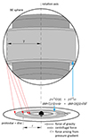Fig. 1. Schematic illustration of the model used. Each gas parcel of the BE sphere whose specific angular momentum falls into a given interval will eventually be accreted onto a ring within the disc, while retaining its angular momentum. As a result of a radial pressure gradient, the specific angular momentum of the gas within the ring can differ from the Keplerian value. The force vectors drawn on the figure give rise to a sub-Keplerian rotation.

3.3. Balance of forces

Assuming a circular motion for each gas parcel, the balance between centrifugal force, gravity, and pressure gradient yields another equation for the structure of the disc. To derive the latter, we start from the Euler equation:

$$\begin{array}{c}\hfill \varrho (\frac{\partial \mathit{v}}{\partial t}+\left(\mathit{v}\mathrm{\nabla }\right)\mathit{v})=-\mathrm{\nabla }p-\varrho \mathrm{\nabla }U,\end{array}$$(12)

where U stands for the gravitational potential. Using cylindrical co-ordinates, for the radial components we have

$$\begin{array}{c}\hfill -\frac{\varrho v^2}{r}=-\frac{\partial p}{\partial r}-\varrho \frac{\partial U}{\partial r}.\end{array}$$(13)

Substituting Ω for $\frac{v}{r}$ and c_s²𝜚 for p, where c_s stands for the isothermal sound speed (which, in our case, is independent of r), we can write

$$\begin{array}{c}\hfill -\varrho r{\mathrm{\Omega }}^2=-c_{\mathrm{s}}^2\frac{\partial \varrho }{\partial r}-\varrho \frac{\partial U}{\partial r},\end{array}$$(14)

which can be integrated with respect to z. Rearranging this equation, we get the following:

$$\begin{array}{c}\hfill \frac{\mathrm{d}\mathrm{\Sigma }}{\mathrm{d}r}=\frac{1}{c_{\mathrm{s}}^2}(r·{\mathrm{\Omega }}^2-\frac{\mathrm{d}U}{\mathrm{d}r})\mathrm{\Sigma }.\end{array}$$(15)

We note that we have used the thin disc approximation, supposing that within the disc, $\frac{\partial U}{\partial r}$ does not depend on z.

3.4. The complete set of equations

The set of Eqs. (10), (11), and (15) must be complemented with an equation for the gravitational potential U and another one for the specific angular momentum. The latter one is

$$\begin{array}{c}\hfill j=r^2·\mathrm{\Omega }.\end{array}$$(16)

To set up an equation for the gravitational potential, some other assumptions are needed, since gravitational forces involve significant contributions from the inner and more massive parts of the resulting configuration, for which our basic assumptions do not hold. We return to this topic in Sect. 4.2.

4. Transformed equations of structure

4.1. Introducing new functions

The basic equations presented in the previous section are difficult to handle in their preliminary form; therefore, it is appropriate to transform the functions to make the equations easier to solve. This is explained below, with further details given in Appendix C.

We have to set an outer boundary for the disc or else Eq. (15) would imply an infinite total mass. In the following, we use the same outer boundary for the disc as for the initial Bonnor–Ebert sphere; namely, the maximum value for the radial co-ordinate, r, is equal to R_BE. The more general case is examined in Sect. 4.5. Because of angular momentum conservation, Ω(R_BE) is equal to ω, which is the initial angular velocity of the Bonnor–Ebert sphere.

We introduce the dimensionless spatial co-ordinate x, which is 0 at r = R_BE and 1 at r = 0,

$$\begin{array}{c}\hfill x=1-\frac{r}{R_{\mathrm{BE}}}.\end{array}$$(17)

At r = R_BE, the value of I(j(r)) is zero while the surface density Σ is not – this makes the derivative $\frac{\mathrm{d}\mathrm{\Omega }}{\mathrm{d}r}$ tend to infinity as r approaches to R_BE (cf. Eq. (11)). Therefore, we must introduce a new function χ(x), which has a finite (but non-zero) derivative at x = 0:

$$\begin{array}{c}\hfill \chi (x)={(1-\frac{j(r(x))}{j_{\max }})}^{\frac{3}{2}}={[1-\frac{{(1-x)}^2}{\omega }\mathrm{\Omega }(R_{\mathrm{BE}}(1-x))]}^{\frac{3}{2}},\end{array}$$(18)

where j_max denotes the maximum specific angular momentum:

$$\begin{array}{c}\hfill j_{\max }=R_{\mathrm{BE}}^2·\omega .\end{array}$$(19)

Instead of Σ(r), I(j) and U(r) we introduce σ(x), Y(χ), and V(x), respectively:

$$\begin{array}{c}\hfill \sigma (x)=ln\frac{\mathrm{\Sigma }(r(x))}{\mathrm{\Sigma }(R_{\mathrm{BE}})}=ln\frac{\mathrm{\Sigma }(R_{\mathrm{BE}}(1-x))}{\mathrm{\Sigma }(R_{\mathrm{BE}})},\end{array}$$(20)

$$\begin{array}{c}\hfill Y(\chi )=I(j(\chi ))=I\left(j_{\max }(1-{\chi }^{2/3})\right),\end{array}$$(21)

$$\begin{array}{c}\hfill V(x)=U(r(x))=U(R_{\mathrm{BE}}(1-x)).\end{array}$$(22)

Instead of Eqs. (11) and (15) we now have

$$\begin{array}{cc}\hfill \frac{\mathrm{d}\chi }{\mathrm{d}x}& =\frac{3}{2}\mathrm{\Sigma }(R_{\mathrm{BE}})\frac{{\chi }^{1/3}}{Y(\chi )}(1-x)e^{\sigma (x)},\hfill \end{array}$$(23)

$$\begin{array}{cc}\hfill \frac{\mathrm{d}\sigma }{\mathrm{d}x}& =-\frac{R_{\mathrm{BE}}^2{\omega }^2}{c_{\mathrm{s}}^2}\frac{{(1-{\chi }^{2/3})}^2}{{(1-x)}^3}-\frac{1}{c_{\mathrm{s}}^2}\frac{\mathrm{d}V}{\mathrm{d}x},\hfill \end{array}$$(24)

with the following initial conditions:

$$\begin{array}{c}\hfill \{\begin{array}{c}\hfill \chi (0)=0,\\ \hfill \sigma (0)=0.\end{array}\end{array}$$(25)

4.2. The gradient of gravitational potential

Since the surface density is expected to rise quickly from the edge of the disc towards the centre, it is reasonable to approximate the gradient of the gravitational potential at a given distance, r, from the centre. This is based on the assumption that the potential gradient was produced by a point mass in the centre, which has a mass equal to the total mass within radius, r; we note, however that in reality, rings with radii greater than r exert an outward gravitational force on the gas at r. On the other hand, rings with smaller radii exert an inward force, which is greater than the gravitational force exerted by an equivalent point mass in the centre. For the gravitational potential of thin rings, we refer to Lass & Blitzer (1983).

The conservation of angular momentum (for the outer part of the disc) allows us to calculate the mass within a given radius r from the value of χ at r. By introducing the function

$$\begin{array}{c}\hfill \zeta (\chi )=\frac{{\int }_0^{1-{\chi }^{2/3}}\left({\int }_0^{\sqrt{1-\epsilon }}F({\xi }_{\max }·\sqrt{\epsilon +z^2})\mathrm{d}z\right)\mathrm{d}\epsilon }{{\int }_0^1\left({\int }_0^{\sqrt{1-\epsilon }}F({\xi }_{\max }·\sqrt{\epsilon +z^2})\mathrm{d}z\right)\mathrm{d}\epsilon },\end{array}$$(26)

which gives the ratio of mass within r(χ) to the total mass, the gradient $\frac{\mathrm{d}V}{\mathrm{d}x}$ can be approximated as

$$\begin{array}{c}\hfill \frac{\mathrm{d}V}{\mathrm{d}x}=-\frac{G{M}_{\mathrm{BE}}\zeta (\chi )}{R_{\mathrm{BE}}{(1-x)}^2}.\end{array}$$(27)

The derivation of the expression for ζ(χ) given by Eq. (26) is explained in Appendix D. The function ζ(χ) for K = 15 is illustrated in Fig. 2.

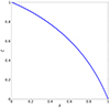Fig. 2. Function ζ(χ) for K = 15.

4.3. Final form of the equations of structure

We can insert the formula given by Eq. (27) into Eq. (24). To express the resulting equation in a more succinct form, we introduced three dimensionless parameters (energy ratios). The value of each is determined solely by ξ_max (or the density ratio K):

$$\begin{array}{c}\hfill \kappa =\frac{E_{\mathrm{BE},\mathrm{rot}}}{M_{\mathrm{BE}}{R}_{\mathrm{BE}}^2{\omega }^2}=\frac{{\int }_0^{{\xi }_{\max }}{\xi }^{4}F(\xi )\mathrm{d}\xi }{3{\xi }_{\max }^2·{\int }_0^{{\xi }_{\max }}{\xi }^{2}F(\xi )\mathrm{d}\xi },\end{array}$$(28)

$$\begin{array}{c}\hfill \lambda =\frac{|E_{\mathrm{BE},\mathrm{grav}}|}{\frac{G{M}_{\mathrm{BE}}^2}{R_{\mathrm{BE}}}}=\frac{{\xi }_{\max }·{\int }_0^{{\xi }_{\max }}({\int }_0^{\xi }\xi \prime {}^{2}F(\xi \prime )\mathrm{d}\xi \prime )\xi F(\xi )\mathrm{d}\xi }{{\left({\int }_0^{{\xi }_{\max }}{\xi }^{2}F(\xi )\mathrm{d}\xi \right)}^2},\end{array}$$(29)

$$\begin{array}{c}\hfill \tau =\frac{|E_{\mathrm{BE},\mathrm{grav}}|}{\lambda M_{\mathrm{BE}}{c}_{\mathrm{s}}^2}=\frac{{\int }_0^{{\xi }_{\max }}{\xi }^{2}F(\xi )\mathrm{d}\xi }{{\xi }_{\max }}.\end{array}$$(30)

The values of ξ_max, κ, λ, and τ for some values of K are given in Table 1. Now Eq. (24) can be written in the following form:

$$\begin{array}{c}\hfill \frac{\mathrm{d}\sigma }{\mathrm{d}x}=\tau (\frac{\zeta (\chi )}{{(1-x)}^2}-\frac{\beta \lambda {(1-{\chi }^{2/3})}^2}{\kappa {(1-x)}^3}),\end{array}$$(31)

with the details of the calculations given in Appendix E.

Equation (23) can also be written in a more succinct form. For this end, we introduce the dimensionless function W(χ) (determined solely by ξ_max) and the constant C:

$$\begin{array}{c}\hfill W(\chi )=\frac{\varrho (0)}{k}\frac{{\chi }^{1/3}}{Y(\chi )},\end{array}$$(32)

$$\begin{array}{c}\hfill C=\frac{3k\mathrm{\Sigma }(R_{\mathrm{BE}})}{2\varrho (0)}.\end{array}$$(33)

We can easily check that

$$\begin{array}{c}\hfill \underset{\chi \to 0^{+}}{lim}W(\chi )=\frac{K}{{\xi }_{\max }}.\end{array}$$(34)

Instead of Eq. (23), we have

$$\begin{array}{c}\hfill \frac{\mathrm{d}\chi }{\mathrm{d}x}=C·W(\chi )(1-x)e^{\sigma (x)}.\end{array}$$(35)

The function W(χ) for K = 15 is displayed in Fig. 3.

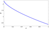Fig. 3. Function W(χ) for K = 15.

4.4. Solution method

As we show above, the equations of structure for the ‘outer’ disc (for which our basic assumptions hold) and the initial conditions can be written as follows:

$$\begin{array}{c}\hfill \{\begin{array}{c}\hfill \frac{\mathrm{d}\sigma }{\mathrm{d}x}=\tau (\frac{\zeta (\chi )}{{(1-x)}^2}-\frac{\beta \lambda {(1-{\chi }^{2/3})}^2}{\kappa {(1-x)}^3}),\\ \hfill \frac{\mathrm{d}\chi }{\mathrm{d}x}=C·W(\chi )(1-x)e^{\sigma (x)},\\ \hfill \chi (0)=0,\\ \hfill \sigma (0)=0.\end{array}\end{array}$$(36)

For each value of the positive parameter C, there is a single solution. It is not possible to take a realistic guess for the value of C a priori. Instead, we can proceed by fixing at first the mass ratio of the ‘outer’ disc to the whole system, thereby obtaining the value of ζ at the inner edge of the ‘outer’ disc. We denote this value using ζ_in (i.e. the mass ratio of the ‘outer’ disc to the whole system is equal to 1 − ζ_in) and the corresponding value of χ by χ_in (i.e. ζ(χ_in) = ζ_in). As a next step, we can fix the ratio of the local angular velocity to the Keplerian one at the inner edge. These two ratios determine C and x_in, the latter denoting the value of the dimensionless co-ordinate at the inner edge (i.e. ζ(χ(x_in)) = ζ(χ_in) = ζ_in). By elevating both ratios simultaneously, we can obtain the same solution, but within an extended domain (with a higher x_in). Thus, it is reasonable to suppose super-Keplerian rotation at the inner edge, namely, to set the angular velocity ratio above unity at x_in to get a full picture of the characteristics of the possible solutions. In this way, we can easily identify the radial distance from the protostar, where the orbital motion of the gas becomes exactly Keplerian. Thus, our model for the ‘outer’ disc can be used as initial condition for protoplanetary disc evolution after truncating the super-Keplerian region and only considering the sub-Keplerian part.

In the following, we use $\frac{\mathrm{\Omega }}{{\mathrm{\Omega }}_{\mathrm{Kep}}}=1.1$ at x_in. Since the centrifugal force is proportional to Ω², this means that the second term on the right-hand side of Eq. (31) is equal to 1.1² = 1.21 times the first term. It follows that

$$\begin{array}{c}\hfill x_{\mathrm{in}}=1-\frac{\beta \lambda {(1-{\chi }_{\mathrm{in}}^{2/3})}^2}{1.21\kappa {\zeta }_{\mathrm{in}}}.\end{array}$$(37)

To obtain the actual value of the constant, C, as well as the functions σ(x) and χ(x), we can use successive approximations; that is, we integrate Eqs. (31) and (35) from x = 0 to x = x_in for different values of C until we find a solution where χ(x_in) = χ_in holds with sufficiently high precision.

To solve Eq. (36), we have written a computer code. For given values of μ, T, K, M_BE, β, and ζ_in, it first determines the values of ξ_max, κ, λ, τ, χ_in, and x_in. Afterward, it starts to integrate the equations of structure from x = 0, using an arbitrary value for C. The numerical integration is performed with a fourth-order Runge-Kutta method. If the value of χ exceeds the value of χ_in before x reaches x_in, the integration is repeated with a smaller value for C. On the other hand, if the value of χ(x_in) stays below χ_in, the integration is repeated with a greater value for C. The integrations are repeated until the obtained value of χ(x_in) differs from χ_in by less than 0.01%. Afterwards, the code transforms the functions χ(x) and σ(x) into Ω(r) and Σ(r). This code is available upon request.

4.5. Exploring the outer boundary

In the previous treatment, we decided the outer boundary of the disc would be located at R_BE. This choice is somewhat arbitrary and it is important to check how sensitive the solutions are to the location of the boundary. Therefore, we can rewrite the equations of structure for the case where the outer boundary is placed at some arbitrary radius, R_out. Thus, we can re-define the dimensionless co-ordinate, x:

$$\begin{array}{c}\hfill x=1-\frac{r}{R_{\mathrm{out}}},\end{array}$$(38)

then we introduce the constant δ for the ratio of the outer radius to that of the Bonnor-Ebert sphere:

$$\begin{array}{c}\hfill \delta =\frac{R_{\mathrm{out}}}{R_{\mathrm{BE}}}.\end{array}$$(39)

The conservation of angular momentum yields an expression for Ω(R_out):

$$\begin{array}{c}\hfill \mathrm{\Omega }\left(R_{\mathrm{out}}\right)=\frac{j_{\max }}{R_{\mathrm{out}}^2}={\left(\frac{R_{\mathrm{BE}}}{R_{\mathrm{out}}}\right)}^2\omega =\frac{\omega }{{\delta }^2}.\end{array}$$(40)

The functions χ(x) and σ(x) will be the following:

$$\begin{array}{cc}\hfill \chi (x)& ={(1-\frac{j(r(x))}{j_{\max }})}^{\frac{3}{2}}={[1-\frac{{\delta }^2{(1-x)}^2}{\omega }\mathrm{\Omega }(R_{\mathrm{out}}(1-x))]}^{\frac{3}{2}},\hfill \end{array}$$(41)

$$\begin{array}{cc}\hfill \sigma (x)& =ln\frac{\mathrm{\Sigma }(r(x))}{\mathrm{\Sigma }(R_{\mathrm{out}})}=ln\frac{\mathrm{\Sigma }(R_{\mathrm{out}}(1-x))}{\mathrm{\Sigma }(R_{\mathrm{out}})}.\hfill \end{array}$$(42)

One of the equations of the structure now reads

$$\begin{array}{c}\hfill \frac{\mathrm{d}\sigma }{\mathrm{d}x}=\frac{\tau }{\delta }(\frac{\zeta (\chi )}{{(1-x)}^2}-\frac{\beta \lambda {(1-{\chi }^{2/3})}^2}{\kappa \delta {(1-x)}^3}).\end{array}$$(43)

Since the constant C can be redefined as

$$\begin{array}{c}\hfill C=\frac{3k\mathrm{\Sigma }(R_{\mathrm{out}}){\delta }^2}{2\varrho (0)},\end{array}$$(44)

the other equation of structure retains its previous form:

$$\begin{array}{c}\hfill \frac{\mathrm{d}\chi }{\mathrm{d}x}=C·W(\chi )(1-x)e^{\sigma (x)},\end{array}$$(45)

while the initial conditions also remain the same:

$$\begin{array}{c}\hfill \sigma (0)=\chi (0)=0.\end{array}$$(46)

To get the solution, we can use the method of successive approximations described in the previous subsection. For x_in, we now have

$$\begin{array}{c}\hfill x_{\mathrm{in}}=1-\frac{\beta \lambda {(1-{\chi }_{\mathrm{in}}^{2/3})}^2}{1.21\kappa \delta {\zeta }_{\mathrm{in}}}.\end{array}$$(47)

It is worth noting that the radius corresponding to x_in does not depend on the location of the outer boundary.

5. Solutions

In the following, we examine three groups of cases (denoted by A, B, and C), each group containing four different subcases. We always suppose initially a Bonnor-Ebert sphere with the following characteristics:

$$\begin{array}{c}\hfill \{\begin{array}{cc}\hfill \mu & =2.3,\hfill \\ \hfill T& =20K,\hfill \\ \hfill K& =15,\hfill \\ \hfill M_{\mathrm{BE}}& =1M_{\odot .}\hfill \end{array}\end{array}$$(48)

We recall here that from the point of view of stability, the critical value of K is about 14.1, namely, the Bonnor-Ebert sphere defined above is slightly supercritical. The corresponding radius and central density of the Bonnor-Ebert sphere are:

$$\begin{array}{c}\hfill \{\begin{array}{cc}\hfill R_{\mathrm{BE}}& =5050\mathrm{AU}\hfill \\ \hfill \varrho (0)& =6.587·{10}^{-18}\frac{\mathrm{g}}{{\mathrm{cm}}^3}\hfill \end{array}.\end{array}$$(49)

The three groups of cases differ in angular velocity, namely, they have different values for β. According to observational data (see Caselli et al. (2002)), β is typically between 10⁻⁴ and 0.07, so we have chosen values from this interval. In group A, the Bonnor-Ebert sphere rotates the slowest, with β = 0.0025. For groups B and C, the value of β is 0.01 and 0.03, respectively. Within each group, each case has a different value for ζ_in. The four cases correspond to ζ_in equal to 0.99, 0.95, 0.85, and 0.75.

5.1. Group A

For the cases in this group, β is equal to 0.0025. The resulting Σ(r) and Ω(r) functions for the four different ζ_in values are presented in Fig. 4. We can see that the four different cases of group A yield practically the same Σ(r) and Ω(r) functions, apart from the lower end of their domains.

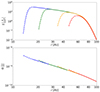Fig. 4. Functions Σ(r) and Ω(r) for β = 0.0025 (Group A). Different colours correspond to different values of ζin. Red: ζin = 0.99, orange: ζin = 0.95, green: ζin = 0.85, and blue: ζin = 0.75.

In each case, the ‘outer’ disc can be divided into three parts or regions. On the log-log plot, the surface density profile increases with rising r in the innermost region, decreases in the middle region, and drops off with a much sharper slope in the outermost region. We note that very far from the centre, the slope becomes smaller again, but this region is not of interest because of its extremely small mass. Passing from one region to another corresponds to a change in the relative magnitudes of the forces acting on the disc matter (cf. Fig. 5, upper panel, for the case with ζ_in = 0.75).

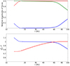Fig. 5. Upper panel: Relative magnitudes of gravity (red), centrifugal force (green) and the force corresponding to pressure gradient (blue). Each magnitude is normalised to the sum of the three. Lower panel: functions ζ(r) (red) and $\frac{\mathrm{\Omega }(r)}{{\mathrm{\Omega }}_{\mathrm{Kep}}(r)}$ (blue). Figures correspond to β = 0.0025 (Group A) and ζin = 0.75.

For small values of r, where rotation is super-Keplerian, Σ(r) rises quickly with growing r. We recall, however, that by setting up the condition expressed by Eq. (37), we artificially ‘enforce’ the emergence of this super-Keplerian region. Hence, in each figure, the super-Keplerian region is presented with a dashed line, highlighting the fact that this region must be truncated in order to fit the ‘outer’ disc to a Keplerian ‘inner’ disc model. In this region, both gravity and the force arising from pressure gradient are directed inwards, together counterbalancing the centrifugal force. For the case with ζ_in = 0.75, the super-Keplerian region extends from 13.33 AU to 17.48 AU (where Ω becomes equal to Ω_Kep) and its mass is about 2% of M_BE (or 8% of the ‘outer’ disc’s total mass). At 17.48 AU, the surface density reaches its maximum value of $1014\frac{\mathrm{g}}{{\mathrm{cm}}^2}$.

The second part of the ‘outer’ disc is characterised by slightly sub-Keplerian rotation. Within this region, surface density diminishes with growing distance from the centre, approximately following a power law (with an exponent between −2 and −3). Centrifugal force and gravity are almost equal in magnitude, while the pressure gradient plays an insignificant role in establishing a balance of forces. For ζ_in = 0.75, the ratio of Ω to Ω_Kep diminishes slowly from unity at 17.48 AU, reaching 0.99 at 53.15 AU. We choose the latter value of r (somewhat arbitrarily) as the upper boundary of the second part of the ‘outer’ disc. This is the region where the bulk of the mass is concentrated: it comprises about 21% of M_BE (or 84% of the ‘outer’ disc’s mass). For comparison, we refer to the ζ(r) function on the lower panel of Fig. 5, where the largest change in the value of ζ occurs in the ‘slightly sub-Keplerian’ region.

For even larger values of r (third region), the rotation of the disc becomes highly sub-Keplerian. The Σ(r) function drops much quicker than before, the force arising from pressure gradient becomes important in counterbalancing gravity. For ζ_in = 0.75, the third region contains 2% of M_BE (8% of the ‘outer’ disc’s mass). Essentially, the disc vanishes around 90 AU: beyond 90.59 AU, ζ approaches unity closer than 10⁻⁶, namely, the mass beyond that radius is only a millionth part of M_BE.

5.2. Group B

For the cases in group B, β is equal to 0.01. The resulting Σ(r) and Ω(r) functions are presented in Fig. 6. Figure 7 illustrates the relative magnitudes of forces as well as ζ and $\frac{\mathrm{\Omega }}{{\mathrm{\Omega }}_{\mathrm{Kep}}}$ as functions of the radial co-ordinate in the case with ζ_in = 0.75.

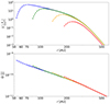Fig. 6. Functions Σ(r) and Ω(r) for β = 0.01 (Group B). Different colours correspond to different values of ζin. Red: ζin = 0.99, orange: ζin = 0.95, green: ζin = 0.85, and blue: ζin = 0.75.

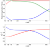Fig. 7. Upper panel: relative magnitudes of gravity (red), centrifugal force (green) and the force corresponding to pressure gradient (blue). Each magnitude is normalised to the sum of the three. Lower panel: functions ζ(r) (red) and $\frac{\mathrm{\Omega }(r)}{{\mathrm{\Omega }}_{\mathrm{Kep}}(r)}$ (blue). Figures correspond to β = 0.01 (Group B) and ζin = 0.75.

The surface density profiles for ζ_in = 0.95, 0.85 and 0.75 essentially converge for large values of r, while the Σ(r) function for ζ_in = 0.99 stays somewhat below the other three. Apart from the latter case, we can still distinguish the three regions of the ‘outer’ disc, but the passage from one region to another is much smoother than in the cases belonging to Group A. As for the Ω(r) functions in the four cases, they all still end up converging at large radii.

In the case with ζ_in = 0.75, the first (super-Keplerian) region is located between 53.18 AU and 71.86 AU, its mass being about 2.7% of M_BE or 11% of the ‘outer’ disc’s mass. After a less dramatic rise than in the corresponding case of Group A, the surface density reaches its peak value of $53.3\frac{\mathrm{g}}{{\mathrm{cm}}^2}$. In the second (‘slightly sub-Keplerian’) region, Σ(r) follows a power law with a similar exponent as in the corresponding case of Group A. However, this time the second region is narrower and much less heavy. The angular velocity drops to 99% of the local Keplerian one already at 92.53 AU, and only 5.4% of M_BE (22% of the ‘outer’ disc’s total mass) is located between 71.86 and 92.53 AU. The rest (16.9% of M_BE, 67% of the ‘outer’ disc’s total mass) is in the third (‘highly sub-Keplerian’) part of the ‘outer’ disc. The third region, in contrast to the second one, is much more extended than in the corresponding case of Group A: ζ approaches unity closer than 10⁻⁶ only beyond 766.7 AU.

5.3. Group C

The fastest initial rotation corresponds to the cases in group C, with β equal to 0.03. The resulting Σ(r) and Ω(r) functions are presented on in Fig. 8. For the relative magnitudes of forces and the ζ(r) and $\frac{\mathrm{\Omega }(r)}{{\mathrm{\Omega }}_{\mathrm{Kep}}(r)}$ functions in the case with ζ_in = 0.75, as shown in Fig. 9.

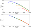Fig. 8. Functions Σ(r) and Ω(r) for β = 0.03 (Group C). Different colours correspond to different values of ζin. Red: ζin = 0.99, orange: ζin = 0.95, green: ζin = 0.85, and blue: ζin = 0.75.

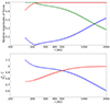Fig. 9. Upper panel: relative magnitudes of gravity (red), centrifugal force (green) and the force corresponding to pressure gradient (blue). Each magnitude is normalised to the sum of the three. Lower panel: Functions ζ(r) (red) and $\frac{\mathrm{\Omega }(r)}{{\mathrm{\Omega }}_{\mathrm{Kep}}(r)}$ (blue). Figures correspond to β = 0.03 (Group C) and ζin = 0.75.

Here, the differences between the Σ(r) profiles corresponding to different values of ζ_in are even more remarkable than in Group B. From the three regions of the ‘outer’ disc, the ‘slightly sub-Keplerian’ one appears to have almost completely disappeared: it is even narrower and lighter than in the cases of Group B. However, the qualitative behaviour of the Ω(r) functions is the same as in Groups A and B.

For ζ_in = 0.75, the super-Keplerian region extends from 159.4 AU to 216.3 AU, reaching at the end a peak surface density of $4.82\frac{\mathrm{g}}{{\mathrm{cm}}^2}$. It contains 2.8% of M_BE (or 11.2% of the ‘outer’ disc’s mass). The ‘slightly sub-Keplerian’ region, between 216.3 AU and 231.8 AU, now contains only 1.2% of M_BE or 4.7% of the ‘outer’ disc’s mass. The ‘highly sub-Keplerian’ region extends from 231.8 AU virtually to the outer boundary of the disc at 5050 AU, its mass being 21% of M_BE (over 84% of the ‘outer’ disc’s mass).

5.4. Qualitative comparison of the three groups of cases

It is hardly surprising that small values of β yield a small disc. The example of Group A has shown that for a small β, the structure of the ‘outer’ part of disc is almost entirely insensitive to the structure of the ‘inner’ part: no matter whether the ‘outer’ disc contains 1% or 25% of the disc matter, its ‘tail’ has the same surface density profile and rotation curve. If the ‘outer’ disc’s mass is not negligibly small, the bulk of this mass moves around the centre with a slightly sub-Keplerian velocity, while the velocity of a small fraction on the ‘edge’ is highly sub-Keplerian. We note, of course, that the small super-Keplerian part can be absent altogether, since each solution can be truncated ‘from within’.

With growing values of β, the size of the disc grows fast. The surface density profile of the ‘outer’ part becomes more sensible to the structure of the ‘inner’ part (but the same cannot be said about the rotation curve at large radii). The ‘highly sub-Keplerian’ region grows together with β at the expense of the ‘slightly sub-Keplerian’ region, which shrinks both in mass and width (not just compared to the whole disc, but also in absolute terms).

5.5. Considering the question of stability

The solutions obtained do not necessarily represent realistic cases that can persist for long timescales, since gravitational instability may produce changes in the disc structure. According to Toomre’s criterion (see Toomre (1964)), instability occurs if Q ⪅ 1, where the dimensionless parameter Q can be calculated as follows:

$$\begin{array}{c}\hfill Q=\frac{c_{\mathrm{s}}{\kappa }_{\mathrm{e}}}{\pi G\mathrm{\Sigma }},\end{array}$$(50)

where κ_e stands for the epicyclic frequency:

$$\begin{array}{c}\hfill {\kappa }_{\mathrm{e}}^2=\frac{2\mathrm{\Omega }}{r}\frac{\mathrm{d}}{\mathrm{d}r}\left(r^2\mathrm{\Omega }\right).\end{array}$$(51)

We have calculated the value of Q as a function of the radial co-ordinate for all the cases examined above. In Group A, only the case with ζ_in = 0.99 is stable on its whole domain. In Group B, there are three fully stable cases (albeit Q gets close to unity in the case with ζ_in = 0.85), while in Group C, due to the lower surface densities, all four cases are stable everywhere. Further details are presented in Table 2.

If the initial assumptions that the collapse is isothermal and angular momentum is being conserved hold for those gas parcels as well, which eventually settle within the unstable region, then at a certain point axial symmetry will break, that may lead eventually to binary or giant planet formation (cf. Boss 1997). Moreover, the resulting gravitational torques will affect the angular momentum transport and, thus, the overall disc structure as well. Hence, the discs in Group B and, especially, Group C seem more self-consistent, than those in Group A. In addition, we may expect that the initial assumptions hold better for the former groups, due to the larger distances from the centre as well as lower densities and angular velocity gradients.

5.6. Changing the outer boundary

In the solutions we have obtained, the bulk of the mass and angular momentum is located within a radius far smaller than R_BE. This suggests that we can displace the outer boundary considerably without seriously affecting the solutions: the effect of the displacement is virtually equivalent to a truncation or an extension of the curves of Σ(r) and Ω(r) obtained for R_out = R_BE.

The numerical solutions of Eqs. (43) and (45) confirm these expectations. We illustrate this in two examples, taken from Groups A and C. From both groups, we chose the cases with ζ_in = 0.75.

The upper panel of Fig. 10 shows the solutions for β = 0.0025, with three largely different outer boundaries, corresponding to δ = 5, δ = 1 and δ = 0.02 (cf. Sect. 4.5). The outer boundaries are located thus at R_out = 25, 250 AU, R_out = 5050 AU and R_out = 101 AU, respectively. (The inner boundary is at the same radius of 13.3 AU in each case.) As we can see, at the given resolution of the figure, the curves overlap; namely, the three solutions match each other almost perfectly. The lower panel of the same figure, which presents the same curves in the close vicinity of the maximum point of Σ(r), confirms that the differences between the solutions obtained for different δ values are indeed extremely small.

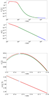Fig. 10. Upper panel: functions Σ(r) and Ω(r) for β = 0.0025 (Group A) and ζin = 0.75 for outer boundaries located at 25 250 AU (blue), 5050 AU (green), and 101 AU (red). Lower panel: Enlarged images of the same functions around the maximum point of Σ(r).

The case of β = 0.03 is somewhat different. In this case, there is more mass and angular momentum in the relatively distant parts of the disc; hence, the solution is more sensitive to the displacement of the outer boundary. Figure 11 shows the solutions for δ = 5, δ = 1, and δ = 0.2; in other words, the outer boundary is located at R_out = 25, 250 AU, R_out = 5050 AU, and R_out = 1010 AU, respectively. The differences between the solutions are clearly visible. However, it is important to note that these differences vanish as we approach the centre, that is: the solutions match each other very well in the densest part of the ‘outer’ disc, where most of its mass is concentrated.

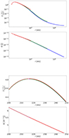Fig. 11. Upper panel: functions Σ(r) and Ω(r) for β = 0.03 (Group C) and ζin = 0.75 for outer boundaries located at 25 250 AU (blue), 5050 AU (green), and 1010 AU (red). Lower panel: enlarged images of the same functions around the maximum point of Σ(r).

6. Comparison with the ‘Keplerian’ infall model

In Takahashi et al. (2013), the authors made the assumption that each infalling gas parcel is accreted onto the disc at a radius where the local Keplerian specific angular momentum is equal to that of the gas parcel and radial pressure gradient plays an insignificant role in establishing a balance of forces. In this work, we examine the conditions under which these assumptions may hold for the outer region of the disc. For this purpose, we calculated the disc structure for different cases using the assumptions of Takahashi et al. (2013), while omitting the angular momentum transport. We note the latter is justified by the fact that we are dealing with a scenario where the outer part of the disc is the least affected by this phenomenon during the collapse phase. After that, we check whether the resulting surface density profiles are consistent with the assumption that the role of pressure gradient is negligible and compare the surface density profiles with those obtained from the calculations presented in this paper.

In the following, we use R_d to denote the disc radius calculated from the assumptions used by Takahashi et al. (2013). For a given initial value of K (or ξ_max) and β, the ratio of R_d to R_BE has a unique value which can be calculated as follows:

$$\begin{array}{cc}\hfill j& =R_{\mathrm{BE}}^2\omega =\sqrt{G{M}_{\mathrm{BE}}{R}_{\mathrm{d}}}\Rightarrow \hfill \\ \hfill R_{\mathrm{d}}& =\frac{R_{\mathrm{BE}}^4}{G{M}_{\mathrm{BE}}}{\omega }^2=\frac{R_{\mathrm{BE}}^4}{G{M}_{\mathrm{BE}}}·\frac{E_{\mathrm{BE},\mathrm{rot}}}{\kappa M_{\mathrm{BE}}{R}_{\mathrm{BE}}^2}=\frac{R_{\mathrm{BE}}^4}{G{M}_{\mathrm{BE}}}·\frac{\beta |E_{\mathrm{BE},\mathrm{grav}}|}{\kappa M_{\mathrm{BE}}{R}_{\mathrm{BE}}^2}\hfill \\ \hfill & =\frac{R_{\mathrm{BE}}^4}{G{M}_{\mathrm{BE}}}·\frac{\beta }{\kappa M_{\mathrm{BE}}{R}_{\mathrm{BE}}^2}·\lambda ·\frac{G{M}_{\mathrm{BE}}^2}{R_{\mathrm{BE}}}=\frac{\beta \lambda }{\kappa }·R_{\mathrm{BE}}\Rightarrow \hfill \\ \hfill \frac{R_{\mathrm{d}}}{R_{\mathrm{BE}}}& =\frac{\beta \lambda }{\kappa }.\hfill \end{array}$$(52)

For a given Σ(r) function, we can calculate the f_p/g ratio between the force arising from pressure gradient and gravity as a function of radial co-ordinate. If f_p/g ≪ 1 holds for most of the mass, then it is justified to neglect the pressure gradient in the model. For a given surface density profile, f_p/g increases with growing radial co-ordinate. If we were to choose some positive value of A, we could calculate the mass, M_A, located beyond a certain radius R_A, for which f_p/g > A. The ratio between M_A and M_BE (as well as the ratio between R_A and R_d) depends solely on K and β.

We numerically calculated the density profile for several values of K and β. We produced a Python code that first generates a BE sphere of a given set of parameters, then divides it into a small inner sphere and 2000 spherical shells, slicing the latter to thin rings perpendicularly to the rotation axis. The shells fall successively onto the disc plane in a way that each ring arrives at a radius where the local Keplerian value of specific angular momentum is equal to the specific angular momentum of the ring. We note that after reaching its place on the disc, each gas parcel remains there, even tough further infall will change the local Keplerian angular velocity.

Table 3 contains the $\frac{R_A}{R_{\mathrm{d}}}$ and $\frac{M_A}{M_{\mathrm{BE}}}$ ratios for A = 0.05 and A = 0.1. The values are calculated for discs originating from the collapse of three types of Bonnor–Ebert spheres: a highly subcritical (K = 2), a slightly supercritical (K = 15) and a highly supercritical (K = 25) one with β = 0.005 (for each value of K) or β = 0.01, 0.02 and 0.03 (only for the supercritical cases).

The data from the table suggest the following. Firstly, for large values of K (i.e. for supercritical BE spheres), $\frac{R_A}{R_{\mathrm{d}}}$ and $\frac{M_A}{M_{\mathrm{BE}}}$ ratios weakly depend on K. Small values of K (highly subcritical BE spheres) also yield similar $\frac{R_A}{R_{\mathrm{d}}}$ ratios as large ones, but the corresponding $\frac{M_A}{M_{\mathrm{BE}}}$ ratios are significantly higher. However, we might not expect the collapse of highly sub-critical BE spheres in this case. Secondly, both the $\frac{R_A}{R_{\mathrm{d}}}$ and $\frac{M_A}{M_{\mathrm{BE}}}$ ratios strongly depend on β. The observed values of β of real cloud cores vary between 10⁻⁴ and 0.07. The role of the pressure gradient becomes significant close to the upper end of this interval, namely, for β ≳ 0.01. As we have seen before, the cases with a high degree of self-consistency are related to these values of β. We shall note, however, that because of rotational flattening, the Bonnor–Ebert sphere becomes a crude approximation of the initial state for large values of β. For a better comparison of the disc structures obtained from the two models, we have plotted the corresponding Σ(r) and ζ(r) functions for the four cases with K = 15 (see Figs. 12 and 13).

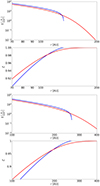Fig. 12. Σ(r) and ζ(r) functions for discs arising from the collapse of a slightly supercritical (K = 15) BE sphere with β = 0.005 (upper panel) and β = 0.01 (lower panel). The red curves correspond to calculations presented in this paper, the blue ones correspond to the ‘Keplerian’ infall model.

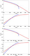Fig. 13. Σ(r) and ζ(r) functions for discs arising from the collapse of a slightly supercritical (K = 15) BE sphere with β = 0.02 (upper panel) and β = 0.03 (lower panel). The red curves correspond to calculations presented in this paper, the blue ones correspond to the ‘Keplerian’ infall model.

7. Summary

Here, we aim to determine the structure of the outer part of a disc arising from the collapse of an unstable, non-magnetic Bonnor–Ebert gas sphere initially rotating as a solid body. If certain conservation laws hold (see Sect. 2), it is possible to derive equations for the disc structure without following up with the collapse process. In our approach, we may lose the ability to follow planet formation processes that might have already started during the collapse of the molecular cloud as the formation of planetesimals, for instance. On the other hand, Drążkowska & Dullemond (2018) have found that planetesimal formation might be uncommon in the disc buildup phase, as it would require very specific conditions.

Our model can be valid only for the less dense, ‘outer’ part of the disc, therefore, our investigations were restricted to this region. The solutions obtained can be fitted to models of the ‘inner’ part of the disc and applied as the initial conditions for the examination of subsequent disc evolution. We note that for this purpose, the solutions can be truncated at an appropriate point, for instance, where Ω is equal to Ω_Kep, or to a slightly sub-Keplerian value, depending on the exponent of power law for the surface density of gas in the inner disc that it is meant to be fitted to.

After describing the basic assumptions of the model (Sect. 2), we set up the structure equations for the ‘outer’ region of the disc in Sect. 3. Since these were difficult to handle, in Sect. 4, we describe how we transformed them to numerically solvable forms by introducing new functions. Once the transformed equations have been integrated, the inverse transformations of the solutions yield the disc’s surface density and angular velocity profiles.

In Sect. 5, we have examined three groups of cases, corresponding to different angular velocities of the initial Bonnor–Ebert spheres. In the case of the slowest rotation, the resulting solutions are quite sharply divided into three regions: a super-Keplerian, a slighly sub-Keplerian, and a highly sub-Keplerian one. We recall here that the presence of a super-Keplerian region is a necessary result of arbitrarily choosing the condition expressed in Eq. (37). It can be considered an artifact and truncated when fitting to a Keplerian ‘inner’ disc model. It is the second region which contains the bulk of the mass. Increasing the angular velocity of the initial BE sphere leads to a fast rise in the resulting disc’s size. At the same time, both the width and the mass of the second region diminish, while the third region grows wide and massive.

A comparison with the ‘Keplerian’ infall model (which supposes that each gas parcel of the collapsing cloud arrives to the disc at the radius where the Keplerian specific angular momentum is equal to that of the gas parcel) in Sect. 6 has shown that for slowly rotating BE spheres, the discs resulting from the two models are very similar; however, there is a considerable difference between the two if the initial BE sphere rotates quickly.

With growing β, the gravitational stability of the disc increases as well, that is, more and more mass is located within the stable region of the disc. The collapse of a slowly rotating BE sphere can lead to an early fragmentation; therefore, by calculating the Toomre parameter, the gravitationally unstable part of the outer disc can be identified, in which giant planet formation might directly begin from the collapsing fragments. On the other hand, from the collapse of a quickly rotating BE sphere, an extended, massive and highly sub-Keplerian disc can emerge, which could play the role of a dust reservoir for planet formation after the disc buildup phase.

Acknowledgments

This research was supported by the NKFIH excellence grant TKP2021-NKTA-64. The authors thank the anonymous reviewer for the useful comments and constructive criticism that helped us considerably improve the manuscript.

References

Appendix A:

The total mass of the Bonnor-Ebert sphere can be calculated as:

$$\begin{array}{c}\hfill M_{\mathrm{BE}}={\int }_0^{R_{\mathrm{BE}}}\varrho (r)4\pi r^2\mathrm{d}r.\end{array}$$

Using ξ = k ⋅ r and 𝜚(r) = 𝜚(0)⋅F(k ⋅ r), we get

$$\begin{array}{c}\hfill M_{\mathrm{BE}}=\frac{4\pi \varrho (0)}{k^3}{\int }_0^{{\xi }_{\max }}{\xi }^{2}F(\xi )\mathrm{d}\xi .\end{array}$$

Using Eq. (5), we can write for k³ the following:

$$k^3=k·k^2=k·\frac{4\pi G\varrho (0)\mu m_{\mathrm{p}}}{k_{\mathrm{B}}T}.$$

The last two equations yield

$$M_{\mathrm{BE}}=\frac{k_{\mathrm{B}}T}{kG\mu m_{\mathrm{p}}}{\int }_0^{{\xi }_{\max }}{\xi }^{2}F(\xi )\mathrm{d}\xi .$$

As a result, we get Eq. (9). The central density of the Bonnor-Ebert sphere can be expressed as follows:

$$\varrho (0)=\frac{M_{\mathrm{BE}}{k}^3}{4\pi {\int }_0^{{\xi }_{\max }}{\xi }^{2}F(\xi )\mathrm{d}\xi }=\frac{{(k_{\mathrm{B}}T)}^3}{4\pi {(G\mu m_{\mathrm{p}})}^3{M}_{\mathrm{BE}}^2}·{\left({\int }_0^{{\xi }_{\max }}{\xi }^{2}F(\xi )\mathrm{d}\xi \right)}^2.$$

Appendix B:

Some small part of the gas cloud was initially at a distance $\stackrel{\sim }{r}$ from the rotation axis. After the collapse, it has a radial co-ordinate, r. The conservation of angular momentum yields

$$j={\stackrel{\sim }{r}}^2\omega =r^2\mathrm{\Omega }\Rightarrow \stackrel{\sim }{r}=\sqrt{\frac{\mathrm{\Omega }}{\omega }}·r.$$

In the initial state, the specific angular momentum interval [j, j + dj] corresponds to an interval $[\stackrel{\sim }{r},\stackrel{\sim }{r}+\mathrm{d}\stackrel{\sim }{r}]$. The relationship between the widths of these intervals can be written as

$$\mathrm{d}j=\frac{\mathrm{d}j}{\mathrm{d}\stackrel{\sim }{r}}\mathrm{d}\stackrel{\sim }{r}=2\stackrel{\sim }{r}\omega \mathrm{d}\stackrel{\sim }{r}\Rightarrow \mathrm{d}\stackrel{\sim }{r}=\frac{\mathrm{d}j}{2\stackrel{\sim }{r}\omega }.$$

The corresponding gas mass dM:

$$\begin{array}{c}\hfill \begin{array}{cc}\hfill \mathrm{d}M& =2\pi \stackrel{\sim }{r}\mathrm{d}\stackrel{\sim }{r}2·{\int }_0^{\sqrt{R^2-{\stackrel{\sim }{r}}^2}}\varrho \left(\sqrt{{\stackrel{\sim }{r}}^2+z^2}\right)\mathrm{d}z=\hfill \\ \hfill & =\mathrm{d}j\frac{2\pi }{\omega }·{\int }_0^{\sqrt{R^2-\frac{j}{\omega }}}\varrho \left(\sqrt{\frac{j}{\omega }+z^2}\right)\mathrm{d}z.\hfill \end{array}\end{array}$$

Using the notation introduced by Eq. (10), we can write

$$\mathrm{d}M=\mathrm{d}j\frac{2\pi }{\omega }I(j).$$

In the final state, the same mass dM is distributed within a radial co-ordinate interval [r, r + dr]. The width of the interval can be calculated as follows:

$$\mathrm{d}j=\frac{\mathrm{d}j}{\mathrm{d}r}\mathrm{d}r=(2r\mathrm{\Omega }+r^2\frac{\mathrm{d}\mathrm{\Omega }}{\mathrm{d}r})\mathrm{d}r\Rightarrow \mathrm{d}r=\frac{\mathrm{d}j}{r·(2\mathrm{\Omega }+r\frac{\mathrm{d}\mathrm{\Omega }}{\mathrm{d}r})}.$$

For the mass dM, we can write

$$\mathrm{d}M=2\pi r\mathrm{d}r\mathrm{\Sigma }=2\pi \mathrm{\Sigma }\frac{\mathrm{d}j}{2\mathrm{\Omega }+r\frac{\mathrm{d}\mathrm{\Omega }}{\mathrm{d}r}}.$$

The two equations for dM yield

$$\mathrm{d}j\frac{2\pi }{\omega }I(j)=2\pi \mathrm{\Sigma }\frac{\mathrm{d}j}{2\mathrm{\Omega }+r\frac{\mathrm{d}\mathrm{\Omega }}{\mathrm{d}r}}.$$

Here, the factor 2πdj cancels out. Re-arranging the equation for $\frac{\mathrm{d}\mathrm{\Omega }}{\mathrm{d}r}$ yields Eq. (11).

Appendix C:

Because of the conservation of angular momentum, the angular velocity of the disc material at R_BE must be the same as the initial angular velocity of the Bonnor-Ebert sphere:

$$R_{\mathrm{BE}}^2·\mathrm{\Omega }(R_{\mathrm{BE}})=R_{\mathrm{BE}}^2·\omega \Rightarrow \mathrm{\Omega }(R_{\mathrm{BE}})=\omega .$$

We must suppose that Σ(R_BE) is not equal to zero, otherwise Eq. (15) yields a constant zero solution for Σ(r). However, Σ(R_BE) > 0 implies that the right hand side of Eq. (11) tends to infinity as r approaches to R_BE. We assume the following approximate form for Ω(r) as r → R_BE⁻:

$$\mathrm{\Omega }(r)\cong \omega -c·\mathrm{\Delta }{r}^{\frac{1}{n}}.$$

Here, c > 0 and n > 1 are constants, while Δr stands for R_BE − r. The corresponding approximate forms for j(r) and I(j(r)) are the following:

$$j(r)\cong R_{\mathrm{BE}}^2·(\omega -c·\mathrm{\Delta }{r}^{\frac{1}{n}})=j_{\max }-R_{\mathrm{BE}}^2·c·\mathrm{\Delta }{r}^{\frac{1}{n}},$$

$$I(j(r))\cong \sqrt{R_{\mathrm{BE}}^2-\frac{j(r)}{\omega }}·\varrho (R_{\mathrm{BE}})\cong \sqrt{c}·R_{\mathrm{BE}}·\varrho (R_{\mathrm{BE}})·\mathrm{\Delta }{r}^{\frac{1}{2n}}.$$

For the two sides of Eq. (11) we have

$$\frac{\mathrm{d}\mathrm{\Omega }}{\mathrm{d}r}\propto \mathrm{\Delta }{r}^{\frac{1}{n}-1},$$

$$\frac{\omega }{r·I(j(r))}·\mathrm{\Sigma }-\frac{2\mathrm{\Omega }}{r}\propto \frac{1}{I(j(r))}\propto \mathrm{\Delta }{r}^{-\frac{1}{2n}}.$$

The two exponents must be equal, which yields the value of n:

$$\frac{1}{n}-1=-\frac{1}{2n}\Rightarrow n=\frac{3}{2}.$$

From these results, it follows that $1-\frac{j(r)}{j_{\max }}\propto \mathrm{\Delta }{r}^{\frac{2}{3}}$. Therefore we introduce the function ${(1-\frac{j(r)}{j_{\max }})}^{\frac{3}{2}}$, which – unlike Ω(r) – has a finite (but non-zero) derivative at R_BE.

Appendix D:

In Sect. 4.2, we introduce the function ζ(χ). For any χ′∈[0, 1], ζ(χ′) is equal to the sum of all mass with χ > χ′, normalised by the total mass of the cloud core. Below, we derive the expression for ζ(χ) given by Eq. (26).

According to Eq. (18), χ > χ′ is equivalent to

$$\begin{array}{c}\hfill j<j^{\prime }=(1-{\chi }^{\prime \frac{2}{3}})·j_{\max }.\end{array}$$

Since the cloud core is supposed to rotate initially as a solid body, one can calculate the mass M′ with j < j′ as the integral of density over the intersection of the Bonnor-Ebert sphere and an infinite cylinder with radius $r\prime =\sqrt{j\prime /\omega }$:

$$\begin{array}{c}\hfill \begin{array}{cc}\hfill M^{\prime }& ={\int }_0^{\sqrt{j^{\prime }/\omega }}\left({\int }_0^{\sqrt{R_{\mathrm{BE}}^2-r^2}}\varrho \left(\sqrt{r^2+z^2}\right)\mathrm{d}z\right)2\pi r\mathrm{d}r=\hfill \\ \hfill & ={\int }_0^{\sqrt{j^{\prime }/\omega }}\left({\int }_0^{R_{\mathrm{BE}}\sqrt{1-r^2/R_{\mathrm{BE}}^2}}\varrho \left(\sqrt{r^2+z^2}\right)\mathrm{d}z\right)2\pi r\mathrm{d}r.\hfill \end{array}\end{array}$$

Instead of r and z, we can introduce the variables $\epsilon =\frac{r^2}{R_{\mathrm{BE}}^2}=\frac{j}{j_{\max }}=1-{\chi }^{\frac{2}{3}}$ and $z\prime =\frac{z}{R_{\mathrm{BE}}}$. Then we have

$$\begin{array}{c}\hfill M^{\prime }={\int }_0^{1-{\chi }^{\prime \frac{2}{3}}}\left({\int }_0^{\sqrt{1-\epsilon }}\varrho \left(\sqrt{\epsilon R_{\mathrm{BE}}^2+z^{\prime 2}{R}_{\mathrm{BE}}^2}\right)R_{\mathrm{BE}}\mathrm{d}{z}^{\prime }\right)\pi R_{\mathrm{BE}}^2\mathrm{d}\epsilon .\end{array}$$

Since 𝜚(r) = 𝜚₀ ⋅ F(k ⋅ r) and k ⋅ R_BE = ξ_max,

$$\begin{array}{c}\hfill \begin{array}{cc}& \varrho \left(\sqrt{\epsilon R_{\mathrm{BE}}^2+z^{\prime 2}{R}_{\mathrm{BE}}^2}\right)=\varrho \left(R_{\mathrm{BE}}\sqrt{\epsilon +z^{\prime 2}}\right)=\hfill \\ \hfill & ={\varrho }_0·F(k·R_{\mathrm{BE}}\sqrt{\epsilon +z^{\prime 2}})={\varrho }_0·F\left({\xi }_{\max }\sqrt{\epsilon +z^{\prime 2}}\right).\hfill \end{array}\end{array}$$

Thus,

$$\begin{array}{c}\hfill M^{\prime }=\pi {\varrho }_0{R}_{\mathrm{BE}}^3{\int }_0^{1-{\chi }^{\prime \frac{2}{3}}}\left({\int }_0^{\sqrt{1-\epsilon }}F\left({\xi }_{\max }\sqrt{\epsilon +z^{\prime 2}}\right)\mathrm{d}{z}^{\prime }\right)\mathrm{d}\epsilon .\end{array}$$

By substituting χ′ = 0, we can get from this formula the whole mass of the Bonnor-Ebert sphere:

$$\begin{array}{c}\hfill M_{\mathrm{BE}}=\pi {\varrho }_0{R}_{\mathrm{BE}}^3{\int }_0^1\left({\int }_0^{\sqrt{1-\epsilon }}F\left({\xi }_{\max }\sqrt{\epsilon +z^{\prime 2}}\right)\mathrm{d}{z}^{\prime }\right)\mathrm{d}\epsilon .\end{array}$$

ζ(χ′) is equal to $\frac{M\prime }{M_{\mathrm{BE}}}$. By dividing the last two expressions above, we get Eq. (26).

Appendix E:

The parameter κ denotes the ratio of the Bonnor-Ebert sphere’s rotational energy E_BE, rot to the product M_BER_BE²ω². Its value is determined by the dimensionless radius ξ_max of the sphere. To calculate it, at first, we introduce the Bonnor-Ebert sphere’s (scalar) moment of inertia I_BE. The value of I_BE can be calculated as the sum of contributions from thin spherical shells, each of which has a uniform mass distribution:

$$\begin{array}{c}\hfill I_{\mathrm{BE}}={\int }_0^{R_{\mathrm{BE}}}\frac{2}{3}{r}^2\varrho (r)4\pi r^2\mathrm{d}r.\end{array}$$

By switching variables, one can transform this equation to

$$\begin{array}{c}\hfill I_{\mathrm{BE}}=\frac{8\pi \varrho (0)}{3k^5}{\int }_0^{{\xi }_{\max }}{\xi }^{4}F(\xi )\mathrm{d}\xi .\end{array}$$

Thus, rotational energy can be written as

$$\begin{array}{c}\hfill E_{\mathrm{BE},\mathrm{rot}}=\frac{1}{2}{I}_{\mathrm{BE}}{\omega }^2=\frac{4\pi \varrho (0)}{3k^5}{\omega }^2{\int }_0^{{\xi }_{\max }}{\xi }^{4}F(\xi )\mathrm{d}\xi .\end{array}$$

Since $\varrho (0)=\frac{M_{\mathrm{BE}}{k}^3}{4\pi {\int }_0^{{\xi }_{\max }}{\xi }^{2}F(\xi )\mathrm{d}\xi }$ (cf. Appendix A) and $k=\frac{{\xi }_{\max }}{R_{\mathrm{BE}}}$ (see Eq. (6)), for the factor $\frac{4\pi \varrho (0)}{3k^5}$ we have

$$\begin{array}{c}\hfill \frac{4\pi \varrho (0)}{3k^5}=\frac{4\pi }{3k^5}·\frac{M_{\mathrm{BE}}{k}^3}{4\pi {\int }_0^{{\xi }_{\max }}{\xi }^{2}F(\xi )\mathrm{d}\xi }=\frac{M_{\mathrm{BE}}{R}_{\mathrm{BE}}^2}{3{\xi }_{\max }^2·{\int }_0^{{\xi }_{\max }}{\xi }^{2}F(\xi )\mathrm{d}\xi }.\end{array}$$

Therefore,

$$\begin{array}{c}\hfill E_{\mathrm{BE},\mathrm{rot}}=\frac{M_{\mathrm{BE}}{R}_{\mathrm{BE}}^2{\omega }^2}{3{\xi }_{\max }^2·{\int }_0^{{\xi }_{\max }}{\xi }^{2}F(\xi )\mathrm{d}\xi }{\int }_0^{{\xi }_{\max }}{\xi }^{4}F(\xi )\mathrm{d}\xi \end{array}$$

$$\begin{array}{c}\hfill \kappa =\frac{E_{\mathrm{BE},\mathrm{rot}}}{M_{\mathrm{BE}}{R}_{\mathrm{BE}}^2{\omega }^2}=\frac{{\int }_0^{{\xi }_{\max }}{\xi }^{4}F(\xi )\mathrm{d}\xi }{3{\xi }_{\max }^2·{\int }_0^{{\xi }_{\max }}{\xi }^{2}F(\xi )\mathrm{d}\xi }.\end{array}$$

We use λ to denote the ratio of the absolute value of gravitational energy to the fraction $\frac{G{M}_{\mathrm{BE}}^2}{R_{\mathrm{BE}}}$. The absolute value of the Bonnor-Ebert sphere’s total gravitational energy can be calculated as follows:

$$\begin{array}{c}\hfill \begin{array}{cc}\hfill |E_{\mathrm{BE},\mathrm{grav}}|& ={\int }_0^{R_{\mathrm{BE}}}\frac{G{\int }_0^r\varrho (r^{\prime })4\pi r^{\prime 2}\mathrm{d}{r}^{\prime }}{r}\varrho (r)4\pi r^2\mathrm{d}r=\hfill \\ \hfill & =\frac{16{\pi }^{2}G{\varrho }^2(0)}{k^5}{\int }_0^{{\xi }_{\max }}\left({\int }_0^{\xi }{\xi }^{\prime 2}F({\xi }^{\prime })\mathrm{d}{\xi }^{\prime }\right)\xi F(\xi )\mathrm{d}\xi =\hfill \\ \hfill & =\frac{{\xi }_{\max }·{\int }_0^{{\xi }_{\max }}\left({\int }_0^{\xi }{\xi }^{\prime 2}F({\xi }^{\prime })\mathrm{d}{\xi }^{\prime }\right)\xi F(\xi )\mathrm{d}\xi }{{\int }_0^{{\xi }_{\max }}{\xi }^{2}F(\xi )\mathrm{d}\xi }·\frac{G{M}_{\mathrm{BE}}^2}{R_{\mathrm{BE}}}.\hfill \end{array}\end{array}$$

Thus, λ is given by the formula

$$\begin{array}{c}\hfill \lambda =\frac{{\xi }_{\max }·{\int }_0^{{\xi }_{\max }}\left({\int }_0^{\xi }{\xi }^{\prime 2}F({\xi }^{\prime })\mathrm{d}{\xi }^{\prime }\right)\xi F(\xi )\mathrm{d}\xi }{{\int }_0^{{\xi }_{\max }}{\xi }^{2}F(\xi )\mathrm{d}\xi }.\end{array}$$

We have defined a third dimensionless parameter, τ, which denotes the ratio of the absolute value of gravitational energy to the product λM_BEc_s². The isothermal sound speed c_s is equal to $\sqrt{\frac{k_{\mathrm{B}}T}{\mu m_{\mathrm{p}}}}$. Using Eqs. (6) and (9), we have

$$\begin{array}{c}\hfill M_{\mathrm{BE}}{c}_{\mathrm{s}}^2=M_{\mathrm{BE}}\frac{k_{\mathrm{B}}T}{\mu m_{\mathrm{p}}}=M_{\mathrm{BE}}k\frac{G{M}_{\mathrm{BE}}}{{\int }_0^{{\xi }_{\max }}{\xi }^{2}F(\xi )\mathrm{d}\xi }=\frac{{\xi }_{\max }}{{\int }_0^{{\xi }_{\max }}{\xi }^{2}F(\xi )\mathrm{d}\xi }·\frac{G{M}_{\mathrm{BE}}^2}{R_{\mathrm{BE}}}.\end{array}$$

Therefore,

$$\begin{array}{c}\hfill \tau =\frac{|E_{\mathrm{BE},\mathrm{grav}}|}{\lambda M_{\mathrm{BE}}{c}_{\mathrm{s}}^2}=\frac{\lambda \frac{G{M}_{\mathrm{BE}}^2}{R_{\mathrm{BE}}}}{\lambda \frac{{\xi }_{\max }}{{\int }_0^{{\xi }_{\max }}{\xi }^{2}F(\xi )\mathrm{d}\xi }·\frac{G{M}_{\mathrm{BE}}^2}{R_{\mathrm{BE}}}}=\frac{{\int }_0^{{\xi }_{\max }}{\xi }^{2}F(\xi )\mathrm{d}\xi }{{\xi }_{\max }}.\end{array}$$

To derive Eq. (31), we depart from Eqs. (24) and (27), making the following transformations:

$$\begin{array}{c}\hfill \begin{array}{cc}\hfill \frac{\mathrm{d}\sigma }{\mathrm{d}x}& =-\frac{R_{\mathrm{BE}}^2{\omega }^2}{c_{\mathrm{s}}^2}\frac{{(1-{\chi }^{2/3})}^2}{{(1-x)}^3}-\frac{1}{c_{\mathrm{s}}^2}(-\frac{G{M}_{\mathrm{BE}}\zeta (\chi )}{R_{\mathrm{BE}}{(1-x)}^2})=\hfill \\ \hfill & =\frac{1}{M_{\mathrm{BE}}{c}_{\mathrm{s}}^2}(\frac{G{M}_{\mathrm{BE}}^2\zeta (\chi )}{R_{\mathrm{BE}}{(1-x)}^2}-M_{\mathrm{BE}}{R}_{\mathrm{BE}}^2{\omega }^2\frac{{(1-{\chi }^{2/3})}^2}{{(1-x)}^3})=\hfill \\ \hfill & =\frac{1}{M_{\mathrm{BE}}{c}_{\mathrm{s}}^2}(\frac{|E_{\mathrm{BE},\mathrm{grav}}|\zeta (\chi )}{\lambda {(1-x)}^2}-E_{\mathrm{BE},\mathrm{rot}}\frac{{(1-{\chi }^{2/3})}^2}{\kappa {(1-x)}^3})=\hfill \\ \hfill & =\frac{1}{\lambda M_{\mathrm{BE}}{c}_{\mathrm{s}}^2}(\frac{|E_{\mathrm{BE},\mathrm{grav}}|\zeta (\chi )}{{(1-x)}^2}-\beta |E_{\mathrm{BE},\mathrm{grav}}|\frac{\lambda {(1-{\chi }^{2/3})}^2}{\kappa {(1-x)}^3})=\hfill \\ \hfill & =\frac{|E_{\mathrm{BE},\mathrm{grav}}|}{\lambda M_{\mathrm{BE}}{c}_{\mathrm{s}}^2}(\frac{\zeta (\chi )}{{(1-x)}^2}-\frac{\beta \lambda {(1-{\chi }^{2/3})}^2}{\kappa {(1-x)}^3})=\hfill \\ \hfill & =\tau (\frac{\zeta (\chi )}{{(1-x)}^2}-\frac{\beta \lambda {(1-{\chi }^{2/3})}^2}{\kappa {(1-x)}^3}).\hfill \end{array}\end{array}$$

All Tables

All Figures

Fig. 1. Schematic illustration of the model used. Each gas parcel of the BE sphere whose specific angular momentum falls into a given interval will eventually be accreted onto a ring within the disc, while retaining its angular momentum. As a result of a radial pressure gradient, the specific angular momentum of the gas within the ring can differ from the Keplerian value. The force vectors drawn on the figure give rise to a sub-Keplerian rotation.

In the text

	Fig. 2. Function ζ(χ) for K = 15.
In the text

	Fig. 3. Function W(χ) for K = 15.
In the text

	Fig. 4. Functions Σ(r) and Ω(r) for β = 0.0025 (Group A). Different colours correspond to different values of ζin. Red: ζin = 0.99, orange: ζin = 0.95, green: ζin = 0.85, and blue: ζin = 0.75.
In the text

	Fig. 5. Upper panel: Relative magnitudes of gravity (red), centrifugal force (green) and the force corresponding to pressure gradient (blue). Each magnitude is normalised to the sum of the three. Lower panel: functions ζ(r) (red) and $\frac{\mathrm{\Omega }(r)}{{\mathrm{\Omega }}_{\mathrm{Kep}}(r)}$ (blue). Figures correspond to β = 0.0025 (Group A) and ζin = 0.75.
In the text

	Fig. 6. Functions Σ(r) and Ω(r) for β = 0.01 (Group B). Different colours correspond to different values of ζin. Red: ζin = 0.99, orange: ζin = 0.95, green: ζin = 0.85, and blue: ζin = 0.75.
In the text

	Fig. 7. Upper panel: relative magnitudes of gravity (red), centrifugal force (green) and the force corresponding to pressure gradient (blue). Each magnitude is normalised to the sum of the three. Lower panel: functions ζ(r) (red) and $\frac{\mathrm{\Omega }(r)}{{\mathrm{\Omega }}_{\mathrm{Kep}}(r)}$ (blue). Figures correspond to β = 0.01 (Group B) and ζin = 0.75.
In the text

	Fig. 8. Functions Σ(r) and Ω(r) for β = 0.03 (Group C). Different colours correspond to different values of ζin. Red: ζin = 0.99, orange: ζin = 0.95, green: ζin = 0.85, and blue: ζin = 0.75.
In the text

	Fig. 9. Upper panel: relative magnitudes of gravity (red), centrifugal force (green) and the force corresponding to pressure gradient (blue). Each magnitude is normalised to the sum of the three. Lower panel: Functions ζ(r) (red) and $\frac{\mathrm{\Omega }(r)}{{\mathrm{\Omega }}_{\mathrm{Kep}}(r)}$ (blue). Figures correspond to β = 0.03 (Group C) and ζin = 0.75.
In the text

	Fig. 10. Upper panel: functions Σ(r) and Ω(r) for β = 0.0025 (Group A) and ζin = 0.75 for outer boundaries located at 25 250 AU (blue), 5050 AU (green), and 101 AU (red). Lower panel: Enlarged images of the same functions around the maximum point of Σ(r).
In the text

	Fig. 11. Upper panel: functions Σ(r) and Ω(r) for β = 0.03 (Group C) and ζin = 0.75 for outer boundaries located at 25 250 AU (blue), 5050 AU (green), and 1010 AU (red). Lower panel: enlarged images of the same functions around the maximum point of Σ(r).
In the text

	Fig. 12. Σ(r) and ζ(r) functions for discs arising from the collapse of a slightly supercritical (K = 15) BE sphere with β = 0.005 (upper panel) and β = 0.01 (lower panel). The red curves correspond to calculations presented in this paper, the blue ones correspond to the ‘Keplerian’ infall model.
In the text

	Fig. 13. Σ(r) and ζ(r) functions for discs arising from the collapse of a slightly supercritical (K = 15) BE sphere with β = 0.02 (upper panel) and β = 0.03 (lower panel). The red curves correspond to calculations presented in this paper, the blue ones correspond to the ‘Keplerian’ infall model.
In the text

References

- Alves, J. F., Lada, C. J., & Lada, E. A. 2001, Nature, 409, 159 [NASA ADS] [CrossRef] [Google Scholar]
- Basu, S. 2015, in IAU General Assembly, 29, 2251914 [Google Scholar]
- Bonnor, W. B. 1956, MNRAS, 116, 351 [NASA ADS] [CrossRef] [Google Scholar]
- Boss, A. P. 1997, Science, 276, 1836 [Google Scholar]
- Caselli, P., Benson, P. J., Myers, P. C., & Tafalla, M. 2002, ApJ, 572, 238 [Google Scholar]
- Chandrasekhar, S. 1939, An Introduction to the Study of Stellar Structure (Chicago: University Of Chicago Press) [Google Scholar]
- Drążkowska, J., & Dullemond, C. P. 2018, A&A, 614, A62 [NASA ADS] [CrossRef] [EDP Sciences] [Google Scholar]
- Ebert, R. 1955, Z. Astrophys., 37, 217 [NASA ADS] [Google Scholar]
- Emden, R. 1907, Gaskugeln (B. G. Teubner) [Google Scholar]
- Hueso, R., & Guillot, T. 2005, A&A, 442, 703 [NASA ADS] [CrossRef] [EDP Sciences] [Google Scholar]
- Iacono, R., & De Felice, M. 2014, Celest. Mech. Dyn. Astron., 118, 291 [Google Scholar]
- Lambrechts, M., & Johansen, A. 2012, A&A, 544, A32 [NASA ADS] [CrossRef] [EDP Sciences] [Google Scholar]
- Lass, H., & Blitzer, L. 1983, Celest. Mech., 30, 225 [Google Scholar]
- Lynden-Bell, D., & Pringle, J. E. 1974, MNRAS, 168, 603 [Google Scholar]
- Machida, M. N., Inutsuka, S.-I., & Matsumoto, T. 2007, ApJ, 670, 1198 [NASA ADS] [CrossRef] [Google Scholar]
- Shu, F. H. 1977, ApJ, 214, 488 [Google Scholar]
- Takahashi, S. Z., Inutsuka, S.-I., & Machida, M. N. 2013, ApJ, 770, 71 [NASA ADS] [CrossRef] [Google Scholar]
- Toomre, A. 1964, ApJ, 139, 1217 [Google Scholar]
- Youdin, A. N., & Goodman, J. 2005, ApJ, 620, 459 [Google Scholar]