| Issue |
A&A
Volume 696, April 2025
|
|
|---|---|---|
| Article Number | A40 | |
| Number of page(s) | 10 | |
| Section | Catalogs and data | |
| DOI | https://doi.org/10.1051/0004-6361/202452886 | |
| Published online | 01 April 2025 | |
3D shape models for describing monolithic asteroids and meteoroids
1
Astronomical Institute of the Czech Academy of Sciences,
Frič ova 298,
25165
Ondřejov, Czech Republic
2
CEITEC – Central European Institute of Technology, Brno University of Technology,
Purkyňova 123,
62100
Brno, Czech Republic
3
Institute of Energetic Materials, Faculty of Chemical Technology, University of Pardubice,
Studentská 95,
53210
Pardubice, Czech Republic
4
Fraunhofer-Institute for High-Speed Dynamics, Ernst-Mach-Institut, EMI,
E.-Zermelo-Str. 4,
79104
Freiburg, Germany
5
Czech Geological Survey,
Geologická 6,
152 00
Prague, Czech Republic
6
Vatican Observatory,
00120,
Vatican City-State, Italy
★ Corresponding author; This email address is being protected from spambots. You need JavaScript enabled to view it.
Received:
5
November
2024
Accepted:
10
February
2025
Abstract
Context. Detailed knowledge of shapes is necessary for modeling certain processes affecting small Solar System bodies, such as the influence of radiative effects – like the YORP effect – on rotation. For meteoroids and small monolithic asteroids, such shapes have not been available up till now. This has strongly limited the possibilities of theoretical studies of the non-gravitational phenomena acting on these bodies.
Aims. Our goal is to create a database of digital 3D shape models that would be suitable for describing the shapes of meteoroids and small monolithic asteroids.
Methods. We performed catastrophic disruption experiments on samples from L3-6 ordinary chondrite NWA 869 and terrestrial tephriphonolite, including one hypervelocity impact and two explosion experiments. We selected fragments with masses of m ≥ 0.2 g that originated from the interior of the samples and did not contain the original target surface. Their size range is approximately 5–24 mm. Their shapes were digitized using X-ray computed tomography, with voxel sizes of about 50 µm.
Results. The resulting database contains 868 shape models in Wavefront OBJ format, as well as a list of the basic properties of each one. The numbers of triangular surface facets of these models range from ∼20 000 to ∼760 000. These shape models correspond to meteoroids and small asteroids created by hypervelocity collisions. When using this database for a particular purpose, it is necessary to consider the selection of appropriate models based on the absence or presence of certain morphological features, such as chondrules, significant cracks, or minor artefacts. The possible presence of these features in a specific shape model has been recorded in the database.
Key words: astronomical databases: miscellaneous / meteorites, meteors, meteoroids / minor planets, asteroids: general
© The Authors 2025
 Open Access article, published by EDP Sciences, under the terms of the Creative Commons Attribution License (https://creativecommons.org/licenses/by/4.0), which permits unrestricted use, distribution, and reproduction in any medium, provided the original work is properly cited.
This article is published in open access under the Subscribe to Open model. This email address is being protected from spambots. You need JavaScript enabled to view it. to support open access publication.
1 Introduction
The shape of the small bodies in the Solar System strongly influences the action of non-gravitational forces and torques, such as the action of escaping gas on small meteoroids during their ejection from a cometary nucleus, the flight of meteoroids through the atmosphere, or radiation-related phenomena. One very important influence comes from the Yarkovsky-O’Keefe-Radzievskii-Paddack (YORP) effect, namely, the emission of thermal radiation from the surface of irregularly shaped bodies that can change the rotational velocity and the direction of the rotation axis (Rubincam 2000). This effect has been detected for 12 asteroids (Ďurech et al. 2024) and it may also be responsible for the breakup of asteroids and the formation of asteroid pairs and binaries. Therefore, it must be considered in the study of the orbital evolution of asteroids given the dependence of the related Yarkovsky effect on the rotational state. In turn, the YORP effect is strongly dependent on the shape and, thus, the prediction of the YORP effect for a particular body is only possible if we know its shape accurately enough – either as a development of the radius vector into spherical harmonics or using a polyhedral description. The approximation of the shape using a dynamically equivalent ellipsoid is entirely insufficient for this purpose. Even convex models created by the light curve inversion method (DAMIT database; Ďurech et al. 2010) do not allow for the YORP effect to be determined for certain bodies.
Detailed models of asteroid shapes are known mainly through spacecraft visits (e.g., Thomas et al. 1996; Daly et al. 2024) or radar observations from Earth (e.g., Ostro et al. 1999; Hudson et al. 2000). For such bodies, it is possible to estimate the magnitude of the YORP effect, although these include some uncertainty on the effect of small irregularities on the surface or the resolution of the surface description (Statler 2009; Breiter et al. 2009). The general properties of the YORP effect and the characteristic timescales have been studied on a large set of artificial shapes: Gaussian random spheres (Vokrouhlický & Čapek 2002; Čapek & Vokrouhlický 2004). These shapes have been constructed in such a way that the surface fluctuations statistically match the shapes of already known asteroids of sizes in the range of ~0.5–15 km (Muinonen & Lagerros 1998).
These results cannot be extrapolated to meteoroids and asteroids smaller than a few hundred meters, which are not rubble-piles, but monolithic instead (Pravec & Harris 2000). This is because (i) for these smaller bodies, there is an effective heat conduction through their volume, which reduces the amplitude of the temperature variations at the surface and, thus, reduces the YORP effect itself; (ii) for monolithic bodies, there is no efficient energy dissipation during non-principal-axis rotation; and (iii) their shapes are different, which is mainly due to their structure. Modeling the YORP effect for small monolithic asteroids and meteoroids is problematic, mainly due to the lack of detailed models of the shapes of these bodies.
The scarcity of information on shapes is also a problem for the study of other non-gravitational phenomena affecting the rotation. However, several attempts have been made in the past to overcome this difficulty. Paddack (1969) considered that the rotation of meteoroids in interplanetary space1 is influenced by a similar effect to YORP, sometimes referred to as the Windmill effect, which is caused by the reflection (scattering) of incident solar radiation. He estimated the torques using a simple hydrodynamic experiment, where he studied the rotation of pieces of gravel sinking to the bottom in a water pool. The rotation of cometary meteoroids caused by gas drag during their ejection from the cometary nucleus under normal activity was studied by Čapek (2014). The unknown meteoroid shapes were substituted by 3D models of terrestrial rock fragments created by low velocity processes (breaking with a hammer or a stone crushing machine in a quarry) and digitized by a laser scanning method. Moreno et al. (2022), when studying a similar problem, replaced the unknown meteoroid shapes with several convex shapes of asteroids derived by the light curve inversion method. Interestingly, they obtained quantitatively similar results as Čapek (2014). The importance of knowledge of the shapes of small meteoroids in modeling their orbital evolution (via the action of direct radiation pressure and the Pointing-Robertson effect) was pointed out by Ryabova (2023).
There is some information currently available on the shapes of meteoroids and small monolithic asteroids. In particular, these bodies have been observed as blocks and particles on the surfaces of some rubble pile asteroids visited by spacecraft, such as Eros, Itokawa, Toutatis, Ryugu, Bennu, and Dimorphos (e.g., Thomas et al. 2002; Michikami et al. 2008, 2019, 2022; DellaGiustina et al. 2019; Li & Zhao 2023). Because it is not possible to observe them from all directions, it is not possible to reconstruct their complete and detailed shapes by photogrammetric methods. They have been described using size ratios in three mutually perpendicular directions, which is insufficient for modeling the above mentioned non-gravitational phenomena. Sample return missions to the asteroids Itokawa, Ryugu, and Bennu allowed the regolith particles to be available for laboratory study. Their digitization by X-ray micro computed tomography (µCT for short) can provide an excellent source of information on meteoroid shapes. However, as far as we know, there is no published catalogue available yet. The shapes of meteoroids and monolithic asteroids can also be inferred using rock fragments from hypervelocity impact experiments (e.g., Michikami et al. 2010; Michikami et al. 2016; Michikami & Hagermann 2021). Even though many hypervelocity impact experiments have been performed and several studies on the shapes of the resulting fragments have been published, we are not aware of any database of shape models that are useful for above-mentioned theoretical studies.
Overall, a database of 3D digital shapes that plausibly describes the common shapes of meteoroids and small asteroids in detail is not yet widely available. This strongly limits the possibility of theoretical studies of some of the non-gravitational phenomena acting on these bodies. Thus, the purpose of this work is the creation of such a database.
In this paper, we describe a method for creating suitable digital shape models and their database and the basic properties of these shapes. Section 2 is devoted to the materials and samples (targets) used. The simulation of meteoroid formation by hypervelocity fragmentation experiments is described in Sect. 3. The selection of suitable fragments and the digitization of their shapes using µCT are discussed in Sect. 4. Finally, in Sect. 5, we describe the shape model database (available at https://shapemodels.asu.cas.cz), along with the morphology of the shapes, a discussion of the distribution of masses and basic shape characteristics, and the advantages and limitations of using the shape models. We have also determined the mean value of the shape factor A, which is important in meteor physics.
2 Samples
The study of meteors and bolides shows that meteoroids entering the atmosphere represent a very diverse population in terms of their composition and mechanical properties. They include iron objects and chondritic ones up to very fragile bodies that have no equivalent among meteorites in the meteorite collections on Earth (e.g., Vojáček et al. 2020; Spurný et al. 2024; Borovička et al. 2020, 2021; Henych et al. 2024; Borovička et al. 2017). It is therefore impossible to select one material for laboratory experiments that matches the entire meteoroid population in terms of its mechanical properties and composition. The same is valid for the material of small monolithic asteroids.
For our experiment, we opted for an ordinary chondrite, both given its lower cost and the greater availability of sufficiently large pieces. This material has a composition similar to that of S-type asteroids or meteoroids producing group I bolides (Ceplecha & McCrosky 1976). Specifically, we used NWA 869, which is an L3-6 ordinary chondrite. We supplemented this primary material with a single sample of terrestrial subvolcanic rock (tephriphonolite) to be able to compare the shapes of fragments from targets with different compositions as well.
The surface of the targets was formed by ablation in the atmosphere, weathering processes, cutting with a diamond saw in the case of NWA 869, and a “low-velocity” separation from the block of rock in the quarry in the case of terrestrial teph-riphonolite. In the experiment, the target was broken by the passage of a shock wave2. Some of the fragments that originated from the surface areas of the targets contained part of the original sample surface that was formed by the processes mentioned above. To distinguish and reject these targets, we painted the surface of each sample white.
2.1 Ordinary chondrite – targets L01 and L02
The NWA 869 meteorite was originally classified as L4-6 ordinary chondrite with shock stage S3 and degree of weathering W1 (Connolly et al. 2006). Metzler et al. (2011) described this material as a coarse-grained L3-6 chondritic regolith breccia, consisting of various types of lithic clasts with different degrees of thermal and shock metamorphism. It contains ~74% of clastic matrix, ~20% of chondrite clasts of petrologic types 5 and 6, shock darkened chondrite clasts, and other minor constituents impact melt rocks, chondrite clasts of petrologic type 3, large NiFe metal grains, and sulfide grains). Metzler et al. (2011) stated that the larger fragments, probably due to their burial in soil during impact, show signs of much more intense weathering. This is also the case of our samples. Flynn et al. (2018) measured the mechanical properties of six samples of NWA 869. They determined a bulk density of 3.36 ± 0.04 g cm−3, grain density of 3.58 ± 0.08 g cm−3, and porosity in the range of 2.7–10.2%, with a mean value of 6.4 ± 2.8%. They noted that the more weathered samples had a lower porosity. The same can be expected for our sample. The unconfined compressive strength of six ~1.5 cm cubes was in range of 52–114 MPa, with a mean value of 87.4 ± 25.6 MPa.
Our sample had an original weight of 1977 g. We first performed an µCT scan, which clearly showed internal cracks and allowed us to design its further cutting. The sample was then cut by diamond saw into three pieces. The sample, designated L01, had dimensions of 10 × 10 × 6 cm and a mass of 853 g, and it was later shattered by a hypervelocity projectile. A cylindrical hole 10 mm in diameter and 12 mm deep was drilled into sample L02. The resulting sample, with dimensions of 10 × 10 × 6 cm, had a mass of 947 g and it was fragmented by an explosive. The remaining piece was used to verify the classification corresponding to NWA 869.
Parameters of fragmentation experiments
2.2 Terrestrial rock – target T01
A terrestrial rock was collected at the former quarry on Kunětická hora (Czech Republic), which exposes laccolith emplaced in older Mesozoic sediments (mainly calcareous clay-stones) in the Late Oligocene (V. Rapprich, personal communication). The rock, a fine-grained porphyritic phonotephrite through to tephriphonolite, contains small phenocrysts of pyroxene (aegirine-augite) as well as, sporadically, of amphibole. The groundmass consists of K-feldspars, acid plagioclase, nepheline, sodalite group minerals, and pyroxene, as well as small amounts of titanite and calcite. Amygdules are also present in the rock and they are mostly filled with zeolites, analcime, and calcite (Kočandrle 1973). The mechanical properties of the rock were previously studied by Hofrichter (1972). The results of this work, which has been lost since, were reported in Kočandrle (1973). Here, we provide the mean value of each quantity and its range in parentheses: density: 2.31 g cm−3 (2.09–2.46 g cm−3), porosity: 13.1% (7.5–22.6%), compressive strength: 108 MPa, (66–167 MPa), tensile strength: 9 MPa (5–24 MPa), and Young’s modulus: 25.7 GPa (11.0–43.1 GPa).
Our sample (referred to as T01) was fresh rock measuring approximately 10 × 8 × 6 cm with no visible signs of weathering and no visible macroscopic fractures. A hole with a diameter of 10 mm and a depth of 10 mm was drilled into the sample. Its weight was 834 g and it was fragmented by an explosive.
3 Hypervelocity fragmentation experiments
Collisions in the main asteroid belt are responsible for asteroids with a rubble pile structure and they also produce smaller monolithic asteroids and meteoroids. Laboratory simulations of these collisions were carried out either by impact of hypervelocity projectiles on suitable targets (e.g., Nakamura & Fujiwara 1991; Flynn et al. 2018) or by shooting the target using an explosive charge (“contact charge technique”, e.g., Giblin et al. 1994). The study of the size, shape, velocity, and rotation distributions of the resulting fragments then makes it possible to achieve a better understanding of the processes in the main asteroid belt (e.g., Giblin et al. 1998).
We also simulate the formation of meteoroids and monolithic asteroids using hypervelocity catastrophic fragmentation of targets (L01, L02, and T01). Both the more sophisticated impact of a hypervelocity projectile and the simpler but cheaper contact charge technique have been used. As shown in Sect. 5, both methods give consistent distributions of fragment sizes and shapes. When designing the experiment, we required (i) that the target should be fragmented into as many fragments as possible and (ii) that the fragments could be digitized in sufficient detail using µCT. A suitable fragment size based on these requirements was estimated to be around 1 cm. Based on Flynn et al. (2018), we then estimated that each of the targets (with low porosity and a mass of slightly less than 1 kg, see Table 1) should receive a specific energy of roughly Q = 10 kJ kg−1.
3.1 Hypervelocity impact fragmentation
Fragmentation of the L01 sample was performed with a hyper-velocity impact at the two-stage light gas gun facility of the Fraunhofer Institut für Kurzzeitdynamik at Ernst-Mach-Institut (EMI). The target was painted white and placed in a chamber whose walls, except for a plexiglass window, were lined with 2 cm thick paper-covered foam. The target was freely placed on the support rod and the chamber was evacuated to 120 mbar. An 8 mm diameter aluminum sphere with a mass of 0.727 g was used as a projectile. The projectile hit the target approximately perpendicular to the surface, in the direction to the center of mass. The impact velocity was 5.6 km s−1, which corresponds to a kinetic energy of 11.4 kJ. The impact velocity was chosen to match the mean impact velocity in the main asteroid belt, which is 5.3 km s−1 (Bottke et al. 1994). During the experiment, a highspeed camera record was taken (see Fig. 1), showing that some of the fragments that hit the plexiglass window have undergone secondary fragmentation. Otherwise, most of the fragments did not have sufficient energy to penetrate the foam and landed at the bottom of the chamber.
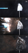 |
Fig. 1 Fragmentation of sample L01 recorded with a high-speed camera: (a) the target and the approaching projectile 0.1 ms before the impact. (b) fragmentation of the target just after the impact. (c) the target fragmented into individual fragments 0.5 ms after the impact. The surface of the target is painted white. |
3.2 Contact charge technique
Samples T01 and L02 were fragmented using the contact charge technique. We used Semtex 1A explosive (83 wt.% penterythritol tetranitrate, 17 wt.% polystyrene-butadiene rubber), which has a detonation velocity of 7.4 km s−1, and a density of 1.47 g cm−3 (Elbeih et al. 2011). Calculated heat of detonation is ~5100 kJ g−1 (e.g., Elbeih et al. 2020).
Considering the sample masses, we chose 1.25 g of explosive for sample T01 and 2.11 g of explosive for sample L02, as can be seen in Table 1. Holsapple (1980) showed that equivalent results can be obtained using an explosive event to simulate impact cratering events, assuming a certain burial depth that is between 1–2 radii of the explosive charge used. Such an arrangement has been used in fragmentation experiments by, for instance, Housen et al. (1991), or Giblin et al. (1994). We used this approach as well. A 10 mm diameter hole was drilled in both samples. The hole depth was 10 mm for sample T01 and 12 mm for sample L02. The surface of the samples was painted white. The experiments was carried out at the KV2 blast chamber at the Institute of Energetic Materials, University of Pardubice. The chamber walls were lined with soft material to minimize the amount of secondary fragmentation. Polystyrene of 5 cm in thickness was covered with a thin aluminium foil and ballistic gelatine, covered with a thin aluminium foil, and then used for the fragmentation of T01. For the L02 fragmentation, 3 cm thick paper-covered foam was used. The explosive charge was pushed into the bottom of the drilled hole, a detonator attached, and the entire sample was then placed approximately in the center of the chamber. We then performed the shot and collected the fragments. Most of the fragments bounced off the walls and were found at the bottom of the chamber, with only minimal amounts penetrating the foam, polystyrene, or ballistic gelatine.
4 Digitization
4.1 Selection and preparation of fragments
After each shot, all material was collected and further sorting was done in the laboratory. As we have stated earlier in this work, we are primarily interested in the shapes of the fragments the surface of which has been shaped by the shock wave passage. Therefore, we excluded all fragments that had part of their surface covered with white paint. Furthermore, we selected only fragments with a mass greater than or equal to 0.20 g. The specific threshold was chosen so that the smallest fragments are approximately 5 mm in size. The shape models of smaller samples could not be detailed sufficiently. Another reason for fixing a specific weight limit was to reduce the possible selection effect caused by the human tendency to preferentially (unintentionally) choose certain shapes. The selection of fragments was done manually using tweezers and laboratory scales with an accuracy of ±0.01 g.
Due to the large total number of fragments, it was not possible to digitize each one separately. Therefore, we digitized them in groups of several tens to hundreds of pieces. For this purpose, the fragments were stacked in boxes made of thin PET-G plastic and fixed with foam to prevent displacement during digitization. Most of the fragments of T01 (except for the largest fragments T01E143 and T01E144) were placed in 210 × 150 × 25 mm box labeled as F. The fragments from L01 and L02 were placed in five cylindrical cases with identical diameters and heights of 70 mm labeled as A, B, C, D, and E. The largest fragments of T01, T01E143 and T01E144, were added to container E. Each case contained several levels separated by foam, and within each level was a thin PET-G grid separating the fragments.
4.2 X-ray computed tomography
The digitization process was carried out by µCT in the Laboratory of X-ray micro and nano computed tomography at CEITEC, Brno University of Technology. Each container (i.e., A, B, C, D, E, and F) was measured separately, so there were a total of six measurements over two campaigns. Due to the size and amount of irradiated material in the containers, the measurements were divided between two instruments in two stages to achieve the best results (see Table 2 for details). The first stage of measurements was performed with a resolution of 46 µm and 55 µm achieved for the second set of measurements. Tomographic measurements were performed at 21° C. The CT system was calibrated before each measurement using a certified phantom with two ruby balls (diameter 10 mm, and spacing 100 mm). The reconstruction of the measured data was performed using the software datos|x 2 reconstruction 2.6.1–RTM. The acquired µCT data were virtually segmented and divided into individual fragments using the software VGStudio Max 2023.3.
The surface determination was performed by determining the isovalue for the material-background boundary based on the histogram of degrees of grey. The histogram typically contains two distinct local maxima, whose positions can be denoted as ɡ1 and ɡ2. The isovalue (treshold value) was chosen as ɡi = ɡ1 + 0.5(ɡ2 − ɡ1) in case of containers A – D, and F. Container E contains fragments of two different compositions (L chondrite and trachybasalt) and the corresponding histogram has four local maxima. In this case, we take the maximum on the far left as ɡ1 and the maximum on the far right as ɡ2. We use a coefficient of 0.5 for the fragments of target L02 and 0.3 for the two large fragments of target T01 (T01E143 and T01E144). Based on this isovalue, the preliminary surface is determined. This surface is refined in the next step using the “advance surface determination” function. This refinement process detects the boundary between the material and the air by identifying the grayscale gradient at their interface. It generates a surface normals based on the threshold value, pinpointing the region with the largest grayscale contrast. The surface can then be interpolated with sub-voxel precision for greater accuracy. These locations then represent the final surface. Its shape is not very sensitive to the particular choice of the initial isovalue. Finally, the individual fragments were exported as STL models with the following export parameters: mode – ray-based; resampling – none; point reduction – precise; and simplification – none.
Parameters of µCT measurements.
4.3 Postprocessing
The resulting shape models are polyhedra with many thousands of triangular surface faces (~20 000–760 000). The models consist of a list of vectors corresponding to each vertex and a list of indices of these vertices forming each triangular face. (In the following text this is referred to as the “mesh”). The meshes of some STL models contain topological defects that can cause problems for 3D analysis software tools. Because of the large number of shapes involved, we did not use MeshLab software (Cignoni et al. 2008) to remove these defects; instead, we developed a script using the PyMeshLab library (Muntoni & Cignoni 2021). As a result, all shape models are produced using the same methodology (with a few exceptions described below) and are reproducible. Our procedure consisted of removing (i) isolated parts, (ii) non-two-manifold edges, (iii) non-two-manifold vertices, (iv) T-vertices, and (v) self-intersecting faces (see Fig. 2). These modifications further required (vi) closing holes in mesh, and (vii) reorienting faces coherently. Most topological defects have one main cause, which is the presence of clearly recognizable cracks. As the crack narrows towards the interior of the fragment, its walls approach each other. Thus, given the finite resolution of the model, it may be the case that the two walls are connected at several locations by a single point or a single edge, resulting in defects (ii) and (iii). The formation of separate cavities (i.e., isolated parts) is also possible during crack closure or in the occurence of self-intersecting faces when triangulation fails locally. Finally, for each of these fixed meshes, a transformation of the coordinate system origin to the center of mass and a rotation to the principal axes of the inertia tensor was performed. The resulting shape model was saved in Wavefront OBJ format.
Each of the shape models created in this way was visually inspected in detail using MeshLab. For several of them, we made additional manual adjustments. Models L01C031a, L01C036a, and T01F028a exhibited misoriented outer normals. Thus, for L01C031a and L01C036a, we skipped step (vii) in the above procedure, however, the T01F028a model still contained self-intersecting faces. We removed them manually in MeshLab, closed the resulting hole in the mesh, and applied the procedure described above to that shape again. We also manually fixed several shape models that contained narrow pyramids on the surface facing the interior of the object. We manually removed these pyramids in MeshLab, closed the resulting holes, and repeated the procedure described above. The resulting shapes are marked with letter “m” in the database. The described mesh repair procedure was finally applied once more for the whole set of shape models in OBJ format. This is because in the ASCII OBJ files the vectors are expressed to six decimal places, whereas the STL files are in binary form. We note that in several cases, this resulted in additional minor network defects due to rounding.
Some shape models contain artifacts – deformations of the surface that arise during digitization. They are caused primarily by the presence of significant material absorption inhomogeneities. In most cases, only a small number of easily recognizable deformations are present (as discussed in Sect. 5.2). The repair of these minor deformations is trivial, but it must be done manually. Because of the significant time consumption required, we postpone this modification for future work. In the current version of the database, we only indicate the presence of these minor artefacts with the note “a” (see Sect. 5.1).
Ultimately, for 47 fragments, it was difficult to correctly determine the shape of the surface. These surfaces exhibited a large number of growths and depressions which do not correspond to reality (see Fig. 3 right). Such shape models are unusable and have been removed from the database. The correction of these cases is possible, but it requires an individual approach to each of them during the processing of the corresponding tomograms, which we leave for future works. Another five shape models were removed from the database because they were found to contain part of the original target surface.
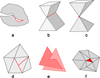 |
Fig. 2 Mesh defects: (a) isolated part, (b) non-two-manifold edge, (c) non-two-manifold vertice, (d) T-vertice, (e) self-intersecting faces, and (f) hole in mesh. |
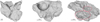 |
Fig. 3 Examples of morphological features on surface of shape models. Left: significant crack in L01C020a. Middle: pit left by a chondrule in L02A117a. Right: significant artefact on L02B005a, which appears as a very bumpy area with alternating holes and growths (marked in red). This shape model was rejected from the database. |
5 Results and discussion
5.1 Database
The database contains a total of 868 shape models suitable for the description of meteoroids and small monolithic asteroids and it is available at https://shapemodels.asu.cas.cz. Each shape model is stored in a separate file in Wavefront OBJ format. The numbers of triangular surface facets range from 20 396 to 758 380 and the histogram can be seen in Fig. 4. The distribution of the mesh edge lengths3 has two peaks (see Fig. 5). The first peak has a median of 0.103 mm and corresponds to shape models of fragments L01, L02, and two fragments T01E143a and T01E144a, which had a voxel size of 46 µm. The second peak has a median of 0.117 mm and corresponds to models of fragments T01 (excluding the two mentioned above), which were scanned with lower resolution (55 µm). The name of each file includes several information. The first three characters of the file name are the designation of the fragmented target (L01, L02, T01). The next character represents the designation of the box in which the fragment was stored during digitization (A, B, C, D, E, and F). The next three characters are its numerical code within that box (e.g., 007, 223). The sequence of these numerical codes may not be continuous for a given box; some digits are skipped. (For example, because the presence of part of the original surface on the fragment was overlooked, as it was subsequently discovered.) The last character corresponds to the way in which the shape was created. In the current version of the database, this is just the “a” character, denoting the method described in Sect. 4. In subsequent versions, there may be shape models of the same fragments, but created by a different process, for example with minor artefacts removed manually, or scanned by a different instrument. The database also contains a text file with a list of all shape models and basic data for each of them:
number of faces;
number of vertices;
genus, a topological quantity that, in simple terms, expresses how many holes4 a given shape has. For example, an ellipsoid has a genus of 0, an anuloid has a genus of 1. Models of shapes that have a higher genus contain cracks, or possibly artifacts, as described in Sect. 4;
size is the diameter of a equal-volume sphere (mm);
dimensions a × b × c. Each shape model is oriented to the principal axes of the inertia tensor. The dimension a is the length in the x-axis direction, b is the length in the y-axis direction, and c is the length in the ɀ-axis direction. Here, a ≥ b ≥ c is considered. These dimensions are in mm;
surface area of the model expressed in mm2;
volume of the model expressed in mm3;
the principal components of the inertia tensor divided by the density. In a principal axis coordinate system, the inertia tensor has non-zero diagonal components only. These components are expressed in mm5. For expression of the inertia tensor in SI units, these values must be multiplied by a factor of 10−12 and by the density;
the average length of the mesh edges in millimetres;
the voxel size in millimetres;
target designation, i.e., L01, L02, or T01;
reference to the article describing the method of obtaining the given shape model;
note may consist of several letters, the meaning of which is as follows: “a” indicates that the shape model contains a small number of insignificant artifacts, “b” indicates the presence of a significant crack, “c” means the presence of a chondrule or a hole after a chondrule emerging at the surface, and “m” means manual modification;
file name.
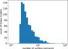 |
Fig. 4 Histogram of the numbers of surface elements of shape models. |
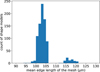 |
Fig. 5 Historgam of mean mesh edge lengths. |
5.2 Morphological features of shape models
Each of the shape models was visually inspected in detail using MeshLab and unusual morphological features were marked. For simplicity, these features are divided into several groups, which are discussed in more detail below. Their identification was made on the basis of a visual and therefore necessarily subjective evaluation. Sometimes it was not possible to decide unambiguously whether or not to mark a given feature on the surface of the shape model. For example, in the case of cracks, it can be uncertain where the boundary between a significant crack (marked with a “b”) and an insignificant crack (which are not marked) lies. For this particular case, it would certainly be possible to find an objective criterion, create an appropriate script and apply it, but that is beyond the scope of this paper.
Significant cracks are present in 101 shape models (see Fig. 3 left). We assume they were formed during the hypervelocity fragmentation experiment. In some cases, they cross almost the entire fragment’s cross-section. Among fragments of terrestrial rock T01, their frequency is roughly double than that of L01 and L02.
Chondrules and the much more common pits left by chondrules have been identified in 24 cases (Fig. 3 middle). They occur only in fragments of L01 and L02; they are of course absent in fragments of terrestrial tephryphonolite. Relatively reliable identification was only possible for chondrules larger than about 1 mm. Smaller structures were mostly not taken into account. As discussed in Sect. 5.6, the use of these models for the description of larger bodies is questionable.
Minor artefacts of various types occur in 383 shape models. This is how we refer to surface features of various origins that cannot be expected on real meteoroids and small monolithic asteroids in space. In most cases, these are holes of varying depth (e.g., Fig. 6). Part of them are produced by the reconstruction of narrow cracks rising to the surface of the fragment due to limited resolution. Others are real and correspond to cavities left by weathered iron grains that are filled with secondary minerals with a lower density and, thus, a lower attenuation (in the case of L01 and L02 fragments); therefore, they are not real artefacts. These structures were formed on Earth due to weathering processes and do not occur on the surfaces of real meteoroids. The shallow holes, sometimes with a rim similar to a small crater, are caused by the presence of iron grains close to the surface and, thus, a large inhomogeneity in density and attenuation. The less frequent growths are probably mostly caused by small loose grain that touches the surface of the fragment. In general, these small artefacts occur approximately twice more frequently in fragments L01 and L02 than in fragments T01.
 |
Fig. 6 Example of a hole in the interior of a shape model L02A105a, corresponding to real hole in the fragment filled by secondary minerals replacing weathered iron grain. The tomogram shows the attenuation (represented by degrees of gray) in the cross section of the corresponding fragment. The white line is the outline of the reconstructed surface. The position of the tomogram is shown in the right corner on the 3D render as the red plane. |
5.3 Mass and shape distribution
The distribution of fragment masses from all three targets can be seen in Fig. 7. The masses are not directly measured on the scales, but calculated from the volume of the corresponding shape model and the density of the material, 3.36 g cm−3 for targets L01 and L02 and 2.31 g cm−3 for target T01. Some masses in Fig. 7 are less than 0. 2 g, although we selected only fragments with masses above 0. 2 g. This is because the actual densities of the fragments are not homogeneous and differ from the above values. The other reason may be that the precision of the scales used in the selection of the samples is 0. 01 g. The cumulative mass distribution has the form N(> m) ∝ m−α. We have determined that for the fragments of targets L01 and L02, α = 1.11 and α = 1.12. A similar value, α = 1.1, was determined by Michikami et al. (2016) for the s2129 shot (Q = 8.54 kJ/kg, mL/mt = 0.018). For fragments of tephriphonolite T01 with less than 1 g we determined α = 0.70. This lower value is close to the value of α = 0.8 that Michikami et al. (2016) obtained for the s2130 shot (Q = 2.47 kJ/kg, mL/mt = 0.088). Targets L01 and L02 are composed of the same material (L3-6 ordinary chondrite), they received similar specific energy (13.3 and 11.4 kJ kg−1), but were fragmented by different methods. Thus, in terms of fragment mass distribution, the two methods are equivalent: explosive charge technique and hypervelocity impact. The different fragment mass distribution of the T01 target may be attributed to the different material, but the more likely cause is a slightly lower degree of fragmentation. We suggest that the selection effect, where we excluded fragments containing part of the original target surface, may affect the resulting mass distribution at lower fragmentation degrees (cratering, core-type fragmentation). However, at a high fragmentation degree (as in our case), we do not expect such an effect, nor do we observe it when we compare our results with earlier experiments where fragment selection was not performed.
Most studies of the shapes of fragments from hypervelocity experiments describe them only in terms of the long, medium, and short axis ratios (a ≥ b ≥ c). As we have already mentioned, such a description is insufficient for the purpose of studying the influence of radiative effects (e.g., YORP) on the rotation of asteroids and meteoroids. However, for comparison purposes, we wanted to see what the distribution of these parameters looks like. Figure 8 shows the Zingg diagram for L01, L02, and T01 fragments. On the x-axis is the flatness ratio c/b (i.e., namely, the ratio of the short to the medium axis) and on the y-axis is the elongation ratio b/a (i.e., the ratio of the medium to the long axis). The mean values (and standard deviations) of the ratios are summarized in Table 3. These values are consistent with the results of previous catastrophic fragmentation experiments, where the mean values of the axial ratios are 2 :  : 1. The same ratio was derived for blocks on the surfaces of some rubble-pile asteroids (e.g., Michikami et al. 2010; Michikami et al. 2022). Based on the statistical t-test, we can say that the shape distributions (defined by the ratios of the individual axes) of the L01 and L02 target fragments are the same at the 0.05 significance level. However, the shape distribution of the T01 target fragments is different (except for the elongation ratio). The lower c/a value indicating a higher abundance of tabular forms is probably caused by a slightly lower degree of fragmentation (Michikami et al. 2016).
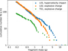 |
Fig. 7 Mass distribution of fragments from the three shots. Horizontal axis show fragment mass m in grams and vertical axis shows the cumulative number of fragments with a mass equal to or higher than m. |
5.4 Shape factor
In the equation for the solar radiation pressure on a meteoroid in space or in equations that describe the motion of a meteoroid in the atmosphere, there is a dimensionless quantity defined as the ratio of the silhouette area, S, of the body and its volume, V, raised to the two-thirds power (Ceplecha et al. 1998):

This parameter depends on the shape of the body and its orientation. In most cases, the simplifying assumption that the body is spherical is used. For such a case, we can derive

A more realistic value of this parameter can be determined by assuming a fast, random rotation of an irregular meteoroid. We used a database of shape models and for each of them we calculated the average value of A over silhouettes with 156 different orientations, uniformly distributed in space5. The resulting distribution can be seen in Fig. 9.
The distributions of 〈A〉 values for the L01 and L02 shape models are the same at the 0.05 significance level and can be approximately described by the mean and standard deviation of 1.58 ± 0.11 and 1.58 ± 0.10. The shape models of the T01 fragments have a distribution with 〈A〉 = 1.67 ± 0.15, which is different from the two distributions above at the 0.05 significance level. We therefore recommend using a value of 1.6 for the shape factor instead of 1 .2, which corresponds to a sphere. This value reflects the shapes of real meteoroids better.
5.5 Difficulties of the method
Despite the attempt to reduce secondary fragmentations by lining the chamber walls with soft material, it is likely that secondary fragmentation has occurred at some level. This is because in some fragments (especially the larger ones), we observe the presence of significant cracks that run through a substantial part of the volume (see Fig. 3 left). It can be assumed that for similar fragments even a slight impact on the soft lining was sufficient to cause disintegration. However, we think that this phenomenon occurred only in a small fraction. Furthermore, we consider that even the fragments produced by secondary fragmentation (and which we cannot distinguish in our database) have shape characteristics identical to those that have not undergone secondary fragmentation. The cracks along which the above mentioned disintegration potentially occurred are also the result of the shock wave propagation through the material, as well as the rest of the surface of the (selected) fragments. The high-speed video shows that several larger fragments of target L01 hit the plexiglass window and shattered. In this case, it is certain that secondary fragmentation occurred.
Another weakness is that despite our method of selecting samples without the original target surface, part of the surface of some fragments may not have been created by the passage of the shock wave. In addition to human mistake (overlooking), there are two reasons how this can happen: (i) detached fusion crust. Among the fragments that do not fulfill the mass criterion m ≥ 0.2 g, we observed several samples represented by a thin shell with one side painted white. These are fusion crust exfoliations. Thus, among the fragments selected for digitization, there are probably samples from whose surface such a shell has detached; (ii) Preexisting cracks. Meteorite NWA 869 used for targets L01 and L02 contained significant cracks visible even visually. In the vicinity of these cracks, more intense weathering processes are evident and their walls may be covered by a thin layer of secondary minerals and, therefore, their morphology is affected by these weathering processes. It is therefore probable that some fragments selected for digitization have parts of their surface formed by a fusion crust exfoliation or a weathering-affected part of the wall of a pre-existing crack. However, it is very difficult to identify such cases specifically. This weakness concerns only the shape models of the L01 and L02 fragments, not T01 fragments.
Thus, in a similar experiment in the future, it would be useful to select a target with a minimal degree of weathering, without the presence of cracks (as was done by Michikami et al. 2024), and trim it into a regular shape, which would both remove the fusion crust and allow easier identification of the fragments containing the target surface. A material with fewer iron and sulfide grains would also be more appropriate to minimize the number of artifacts.
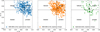 |
Fig. 8 Distribution of shapes. On the x-axis is the ratio of the short to the medium axis and on the y-axis is the ratio of the medium to the long axis. |
Distribution of shapes.
5.6 Application specifics
Some shape models of fragments L01 and L02 contain surface features caused by chondrules. The use of such models for larger bodies, such as small monolithic asteroids, can be problematic because the rescaling will enlarge the corresponding spherical features, which have no real analogue at larger scales. It is therefore better to use shape models that are not marked with a letter “c” for these purposes.
Artifacts are often found among the shape models of fragments L01 and L02 (see Sect. 4.3). It is always necessary to consider whether or not these minor deformations of a small part of the surface may be problematic for the given purpose. Alternatively, shape models without these artefacts, i.e. without the note “a”, could be selected from the database. For some shape models, a certain type of artefact has been manually removed (noted as “m” in the database).
It should also be taken into account that between fragments L01 and L02, there are a small number of samples whose surface may have been partly shaped by a process other than the passage of a shock wave (see Sect. 5.5). The corresponding shape models are not marked in any way in the database. We do not expect such cases for the T01 fragments.
The shape models describe well small monolithic asteroids and meteoroids that were produced by hypervelocity catastrophic fragmentation. However, Michikami et al. (2016) showed that the distribution of fragment shapes depends on the impact energy on the target mass. Therefore, fragments produced by impact cratering will have a different shape distribution. In such a case, the mean value of the ratio of the small and large axes may drop to a value of c/a = 0.2. For a similar reason, the use of the shape database for cometary meteoroids and meteoroids formed by even less energetic or low-velocity processes such as thermal stresses (Čapek et al. 2022; Koten et al. 2024) may be put into question.
It must also be noted that the shapes of these bodies are not constant, but evolve due to the erosive effects of collisions with interplanetary dust particles or due to thermal stresses (Delbo et al. 2014; Molaro et al. 2017). Thus, the original sharp-edged fragments can be expected to become more rounded over time.
If we take into account the specifics described above (e.g., excluding shape models affected by chondrules), they can be used for a more accurate statistical characterization of the YORP effect on small monolithic asteroids. This is because the shape models match the small monolithic asteroids better than the Gaussian random spheres that have been used for the statistical study of YORP on rubble-pile asteroids (Vokrouhlický & Čapek 2002).
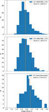 |
Fig. 9 Distribution of shape factor 〈A〉. The dashed vertical line denotes the value for the spherical body. |
5.7 Future work and database expansion
We expect that the database will continue to expand: the described fragments were also scanned with another µCT device at the Faculty of Electrical Engineering of the Czech Technical University in Prague. When we finish the digitization and postprocessing of the shape models, we will add them to the database. It will be interesting to compare them with the current models and estimate the accuracy of the surface determination. Next, we plan to manually remove minor artefacts that occur on some of the current shape models and add these modified shape models to the database.
Using the same method described above, ~200 shapes of fragments of H6 ordinary chondrite (currently without an official name) have been created. We have not included them in the current version of the database to avoid reducing its credibility and usability. If we succeed in the approval of the official name of the used meteorite, we will expand the database with these shape models.
Finally, we plan to create fragments using various “low speed” processes. Their shapes may be useful for describing meteoroids that were not created by an impact process but, for example, via the action of thermal stresses.
Data availability
The shape models and metadata are available on the database website at https://shapemodels.asu.cas.cz/, or on Zenodo at https://doi.org/10.5281/zenodo.14850374.
Acknowledgements
Jonáš Čapek, Šimon Čapek, Eliška Hanušová, Tereza Zichová for their help with the sorting of the fragments, and Václav Rapprich for information on the terrestrial rock. We also thank an anonymous reviewer for helpful comments. This work was supported by the Grant Agency of the Czech Republic grant 20-10907S and by institutional project RVO:67985815. We also acknowledge CzechNanoLab Research Infrastructure supported by MEYS CR (LM2023051). J.K. thanks to the support of grant FSI-S-23-8389 / support of the Faculty of Mechanical Engineering at the Brno University of Technology.
References
- Borovička, J., Spurný, P., Grigore, V. I., & Svoreň, J. 2017, Planet. Space Sci., 143, 147 [CrossRef] [Google Scholar]
- Borovička, J., Spurný, P., & Shrbený, L. 2020, AJ, 160, 42 [CrossRef] [Google Scholar]
- Borovička, J., Bettonvil, F., Baumgarten, G., et al. 2021, Meteor. Planet. Sci., 56, 425 [CrossRef] [Google Scholar]
- Bottke, W. F., Nolan, M. C., Greenberg, R., & Kolvoord, R. A. 1994, Icarus, 107, 255 [NASA ADS] [CrossRef] [Google Scholar]
- Breiter, S., Bartczak, P., Czekaj, M., Oczujda, B., & Vokrouhlický, D. 2009, A&A, 507, 1073 [NASA ADS] [CrossRef] [EDP Sciences] [Google Scholar]
- Čapek, D. 2014, A&A, 568, A39 [NASA ADS] [CrossRef] [EDP Sciences] [Google Scholar]
- Capek, D., & Vokrouhlický, D. 2004, Icarus, 172, 526 [CrossRef] [Google Scholar]
- Čapek, D., Koten, P., Spurný, P., & Shrbený, L. 2022, A&A, 666, A144 [NASA ADS] [CrossRef] [EDP Sciences] [Google Scholar]
- Ceplecha, Z., & McCrosky, R. E. 1976, J. Geophys. Res., 81, 6257 [NASA ADS] [CrossRef] [Google Scholar]
- Ceplecha, Z., Borovička, J., Elford, W. G., et al. 1998, Space Sci. Rev., 84, 327 [NASA ADS] [CrossRef] [Google Scholar]
- Cignoni, P., Callieri, M., Corsini, M., et al. 2008, in Eurographics Italian Chapter Conference, eds. V. Scarano, R. D. Chiara, & U. Erra (The Eurographics Association) [Google Scholar]
- Connolly, H. C., Jr., Zipfel, J., Grossman, J. N., et al. 2006, Meteor. Planet. Sci., 41, 1383 [NASA ADS] [CrossRef] [Google Scholar]
- Daly, R. T., Ernst, C. M., Barnouin, O. S., et al. 2024, Planet. Sci. J., 5, 24 [Google Scholar]
- Delbo, M., Libourel, G., Wilkerson, J., et al. 2014, Nature, 508, 233 [Google Scholar]
- DellaGiustina, D. N., Emery, J. P., Golish, D. R., et al. 2019, Nat. Astron., 3, 341 [Google Scholar]
- Ďurech, J., Sidorin, V., & Kaasalainen, M. 2010, A&A, 513, A46 [Google Scholar]
- Ďurech, J., Vokrouhlický, D., Pravec, P., et al. 2024, A&A, 682, A93 [NASA ADS] [CrossRef] [EDP Sciences] [Google Scholar]
- Elbeih, A., Pachman, J., Trzciński, W. A., et al. 2011, Propellants Explosives Pyrotechnics, 36, 433 [Google Scholar]
- Elbeih, A., Hussein, A. K., Elshenawy, T., et al. 2020, Defence Technol., 16, 487 [Google Scholar]
- Flynn, G. J., Durda, D. D., Patmore, E. B., et al. 2018, Planet. Space Sci., 164, 91 [NASA ADS] [CrossRef] [Google Scholar]
- Giblin, I., Martelli, G., Smith, P. N., et al. 1994, Icarus, 110, 203 [Google Scholar]
- Giblin, I., Martelli, G., Farinella, P., et al. 1998, Icarus, 134, 77 [Google Scholar]
- Henych, T., Borovička, J., Vojáček, V., & Spurný, P. 2024, A&A, 683, A229 [NASA ADS] [CrossRef] [EDP Sciences] [Google Scholar]
- Hofrichter, P. 1972, Fysikálně mechanické vlastnosti hornin. Kunětická hora. (in Czech), Technical report, Arch. ONV Pardubice [Google Scholar]
- Holsapple, K. A. 1980, Lunar Planet. Sci. Conf. Proc., 3, 2379 [Google Scholar]
- Housen, K. R., Schmidt, R. M., & Holsapple, K. A. 1991, Icarus, 94, 180 [Google Scholar]
- Hudson, R. S., Ostro, S. J., Jurgens, R. F., et al. 2000, Icarus, 148, 37 [Google Scholar]
- Kočandrle, J. 1973, in Práce a studie Krajského střediska státní památkové péče a ochrany přírody Východočeského kraje: ochrana přírody a krajiny, 5, Geologie Kunětické hory. (in Czech), ed. P. Rybář, 11 [Google Scholar]
- Koten, P., Čapek, D., Midtskogen, S., et al. 2024, A&A, 683, A5 [NASA ADS] [CrossRef] [EDP Sciences] [Google Scholar]
- Li, Y., & Zhao, Y. 2023, Sol. Syst. Res., 57, 495 [Google Scholar]
- Metzler, K., Bischoff, A., Greenwood, R. C., et al. 2011, Meteor. Planet. Sci., 46, 652 [NASA ADS] [CrossRef] [Google Scholar]
- Michikami, T., & Hagermann, A. 2021, Icarus, 357, 114282 [Google Scholar]
- Michikami, T., Nakamura, A. M., Hirata, N., et al. 2008, Earth Planets Space, 60, 13 [NASA ADS] [Google Scholar]
- Michikami, T., Nakamura, A. M., & Hirata, N. 2010, Icarus, 207, 277 [Google Scholar]
- Michikami, T., Hagermann, A., Kadokawa, T., et al. 2016, Icarus, 264, 316 [Google Scholar]
- Michikami, T., Honda, C., Miyamoto, H., et al. 2019, Icarus, 331, 179 [NASA ADS] [CrossRef] [Google Scholar]
- Michikami, T., Hagermann, A., Morota, T., et al. 2022, Icarus, 381, 115007 [Google Scholar]
- Michikami, T., Hagermann, A., Tsuchiyama, A., et al. 2024, Icarus, 415, 116068 [Google Scholar]
- Molaro, J. L., Byrne, S., & Le, J. L. 2017, Icarus, 294, 247 [CrossRef] [Google Scholar]
- Moreno, F., Guirado, D., Muñoz, O., et al. 2022, MNRAS, 510, 5142 [NASA ADS] [CrossRef] [Google Scholar]
- Muinonen, K., & Lagerros, J. S. V. 1998, A&A, 333, 753 [NASA ADS] [Google Scholar]
- Muntoni, A., & Cignoni, P. 2021, https://doi.org/10.5281/zenodo.4438750 [Google Scholar]
- Nakamura, A., & Fujiwara, A. 1991, Icarus, 92, 132 [Google Scholar]
- Ostro, S. J., Pravec, P., Benner, L. A. M., et al. 1999, Science, 285, 557 [NASA ADS] [CrossRef] [PubMed] [Google Scholar]
- Paddack, S. J. 1969, J. Geophys. Res., 74, 4379 [NASA ADS] [CrossRef] [Google Scholar]
- Pravec, P., & Harris, A. W. 2000, Icarus, 148, 12 [NASA ADS] [CrossRef] [Google Scholar]
- Rubincam, D. P. 2000, Icarus, 148, 2 [Google Scholar]
- Ryabova, G. O. 2023, Vestnik Tomskogo Gosudarstvennogo Universiteta Matem- atika i Mekhanika, 83, 151 [Google Scholar]
- Spurný, P., Borovička, J., Shrbený, L., Hankey, M., & Neubert, R. 2024, A&A, 686, A67 [CrossRef] [EDP Sciences] [Google Scholar]
- Statler, T. S. 2009, Icarus, 202, 502 [NASA ADS] [CrossRef] [Google Scholar]
- Thomas, P. C., Belton, M. J. S., Carcich, B., et al. 1996, Icarus, 120, 20 [NASA ADS] [CrossRef] [Google Scholar]
- Thomas, P., Joseph, J., Carcich, B., et al. 2002, Icarus, 155, 18 [NASA ADS] [CrossRef] [Google Scholar]
- Vojáček, V., Borovička, J., Spurný, P., & Čapek, D. 2020, Planet. Space Sci., 184, 104882 [CrossRef] [Google Scholar]
- Vokrouhlický, D., & Čapek, D. 2002, Icarus, 159, 449 [CrossRef] [Google Scholar]
Strictly speaking, the study examined the rotation of tektites in space.
The fragmentation process is more complex and includes the expansion of the explosion or impact products, the interaction of the shock wave with the free surface and the propagation of the rarefaction wave. For simplicity, however, we use this expression in the following text.
Edge length is the distance between two connected vertices.
Please note that these are holes in the body and shape model. They are not holes in the mesh, i.e., topological defects.
For some simple solids, the following values of A were obtained: 1.50 for a cube, 1.56 for a block with an axial ratio of 1 : 0.7 : 0.5, and 1.29 for an ellipsoid with an axial ratio of 1 : 0.7 : 0.5.
All Tables
All Figures
|
Fig. 1 Fragmentation of sample L01 recorded with a high-speed camera: (a) the target and the approaching projectile 0.1 ms before the impact. (b) fragmentation of the target just after the impact. (c) the target fragmented into individual fragments 0.5 ms after the impact. The surface of the target is painted white. |
| In the text | |
|
Fig. 2 Mesh defects: (a) isolated part, (b) non-two-manifold edge, (c) non-two-manifold vertice, (d) T-vertice, (e) self-intersecting faces, and (f) hole in mesh. |
| In the text | |
|
Fig. 3 Examples of morphological features on surface of shape models. Left: significant crack in L01C020a. Middle: pit left by a chondrule in L02A117a. Right: significant artefact on L02B005a, which appears as a very bumpy area with alternating holes and growths (marked in red). This shape model was rejected from the database. |
| In the text | |
|
Fig. 4 Histogram of the numbers of surface elements of shape models. |
| In the text | |
|
Fig. 5 Historgam of mean mesh edge lengths. |
| In the text | |
|
Fig. 6 Example of a hole in the interior of a shape model L02A105a, corresponding to real hole in the fragment filled by secondary minerals replacing weathered iron grain. The tomogram shows the attenuation (represented by degrees of gray) in the cross section of the corresponding fragment. The white line is the outline of the reconstructed surface. The position of the tomogram is shown in the right corner on the 3D render as the red plane. |
| In the text | |
|
Fig. 7 Mass distribution of fragments from the three shots. Horizontal axis show fragment mass m in grams and vertical axis shows the cumulative number of fragments with a mass equal to or higher than m. |
| In the text | |
|
Fig. 8 Distribution of shapes. On the x-axis is the ratio of the short to the medium axis and on the y-axis is the ratio of the medium to the long axis. |
| In the text | |
|
Fig. 9 Distribution of shape factor 〈A〉. The dashed vertical line denotes the value for the spherical body. |
| In the text | |
Current usage metrics show cumulative count of Article Views (full-text article views including HTML views, PDF and ePub downloads, according to the available data) and Abstracts Views on Vision4Press platform.
Data correspond to usage on the plateform after 2015. The current usage metrics is available 48-96 hours after online publication and is updated daily on week days.
Initial download of the metrics may take a while.