| Issue |
A&A
Volume 696, April 2025
|
|
|---|---|---|
| Article Number | A69 | |
| Number of page(s) | 9 | |
| Section | Planets, planetary systems, and small bodies | |
| DOI | https://doi.org/10.1051/0004-6361/202452445 | |
| Published online | 04 April 2025 | |
Towards a definition of a meteor cluster
Detection of meteor clusters from meteor orbit databases
1
LTE, Observatoire de Paris, Université PSL, Sorbonne Université, Université de Lille, LNE, CNRS,
61 Avenue de l’Observatoire,
75014
Paris,
France
2
Astronomical Institute of the Czech Academy of Sciences,
Fricova 298,
25165
Ondřejov, Czech Republic
★ Corresponding author; This email address is being protected from spambots. You need JavaScript enabled to view it.
Received:
1
October
2024
Accepted:
20
February
2025
Abstract
Context. As of today, there is no official definition of a meteor cluster. It is usually identified as a large number of meteors sharing a similar radiant and velocity, all occurring within a few seconds. Only eight clusters have been reported so far, from single-camera or camera network observations. However, a cluster may be observed by several distant networks and remain unnoticed simply because each network is recording a small portion of the cluster.
Aims. We aim to provide an overview of meteor clusters to help define what constitutes a cluster by potentially adding more to the already identified ones and determining their common parameters.
Methods. A search for new clusters was performed in publicly available International Astronomical Union meteor databases with the DBSCAN algorithm. Then, a statistical significance method was applied to derive the most promising cluster candidates. However, the method still lacks a way to debias the atmospheric area surveyed by the cameras due to a lack of publicly available data.
Results. A set of 16 statistically significant potential clusters is identified, involving four to seven fragments. The 90th percentile includes a duration of 8 seconds, a velocity difference of 2.2 km/s, and a radiant spread of nearly 4 degrees. The velocity difference may arise from the method used for orbit computation.
Conclusions. Meteor clusters might be more frequent than currently reported. However, we recommend that future meteor orbit databases also include a way to estimate the surveyed area by the cameras involved in the detection. This would strengthen the veracity of the 16 identified cluster candidates and ultimately allow scientists to fully debias the number of clusters, and hence derive the physical lifetime expectancy of meteoroids, which is often overlooked due to the focus on collisional lifetime estimates only. We also recommend that any future cluster observation report include the expected number of random occurrences and consider the event to be real if this value is below 0.1.
Key words: interplanetary medium / meteorites, meteors, meteoroids
© The Authors 2025
 Open Access article, published by EDP Sciences, under the terms of the Creative Commons Attribution License (https://creativecommons.org/licenses/by/4.0), which permits unrestricted use, distribution, and reproduction in any medium, provided the original work is properly cited.
This article is published in open access under the Subscribe to Open model. This email address is being protected from spambots. You need JavaScript enabled to view it. to support open access publication.
1 Introduction
Meteor showers are characterized by a relatively high number of meteors sharing a similar radiant and occurring over a time span ranging from a few hours to a few weeks (Koten et al. 2019; Williams et al. 2019). During such showers, meteor clusters are rarely seen. A meteor cluster is characterized by a relatively high number of meteors sharing a similar radiant and velocity, occurring within a time interval of a few seconds. Until today, only eight clusters were reported (Hapgood & Rothwell 1981; Piers & Hawkes 1993; Kinoshita et al. 1999; Watanabe et al. 2002, Watanabe et al. 2003; Koten et al. 2017; Vaubaillon et al. 2023; Koten et al. 2024). However, the recognition of clusters is impaired by the lack of an official definition, caused by the scarce frequency of the phenomenon. Another cause of the absence of further detections of meteor clusters is the meteor detection software, which was not explicitly designed for this purpose (Bednář et al. 2023).
Yet, the existence of meteor clusters is an indicator of meteoroid fragmentation in interplanetary space. The most likely physical origin is the thermal stress endured by the meteoroid (Capek et al. 2022). Determining the frequency of such self-fragmentation directly impacts estimates of meteoroid physical lifetimes in interplanetary space. In particular, if the frequency is found to be higher than already suspected, this could explain, for example, the absence of the 2006 Leonids outburst (Jenniskens et al. 2008). This physical lifetime expectancy is often overlooked, in favor of collisional lifetime expectancy (Koschny et al. 2017; Soja et al. 2019). Thus, determining the frequency of meteoroid self-fragmentation by the detection of meteor clusters has implications for the interpretation of meteor shower observations in general. The scientific question this paper seeks to address is whether there are more meteor clusters hidden in the meteor orbit databases than are currently known.
A recent search for additional meteor pairs among the Geminids recorded by the Ondřejov observatory video meteor database (Koten et al. 2021) was performed by Ďurišová et al. (2023). The results show that no cluster was detected, given the data and the statistical significance of the pair candidates. This statistical analysis is crucial, since, as is pointed out by the authors, a simple Poisson distribution underestimates the expected number of clusters in a given database of meteor orbits.
However, all currently known clusters and search for clusters focus on detection with a limited number of cameras (often restricted to just one). The interpretation (Čapek et al. 2022) is that a meteoroid self-fragments in space, and the subsequent non-gravitational forces (highly dependent on the size) cause a slow increase in the physical distance between the different fragments. The measured maximal physical distance between the fragments constrain the maximum time duration between the self-fragmentation of the observation in the Earth’s atmosphere. The maximal physical distance of the analysed clusters was estimated to be a few hundred kilometres, and the corresponding duration since self-fragmentation does not exceed a few days at most (Koten et al. 2017, 2024).
However, the studied clusters were detected either by a single camera or by a network of cameras, surveying a rather small portion of the atmosphere. Now, supposing a simple scenario of a meteoroid self-fragmenting into two pieces (i.e. the most basic cluster possible), and supposing that the self-fragmentation happens a few months before the fragments enter the Earth’s atmosphere, and that the physical distance is 3000 km at the time of the observation: such a distance would make it impossible for this cluster to be detected by a two-camera-network (since cameras of a given network are usually separated by ~ 100 km).Even a network of 100 cameras covering 106 km2 cannot detect such a cluster. However, the two meteors can be detected by two meteor observation networks a few thousand kilometres apart. In this case, the two meteors associated with the atmospheric entry of the two fragments will be detected, but the link between these two meteors cannot be performed, unless the data are available.
The goal of this paper is to examine the current publicly available databases, find potential meteor clusters, and perform a statistical analysis to evaluate their respective relevance. Since there is no current definition of a meteor cluster, it may be tempting to define constraints to help identify future clusters. However, such a procedure might unintentionally set limits that are too strong, preventing future works from providing scientifically sound results. Instead, we aim to provide preliminary statistics of the cluster candidates. It is worth mentioning that the consequences regarding the physical lifetime expectancy are out of the scope of this preliminary study, since this is the topic of thorough research.
The paper first describes the method in Section 2 (including the description of the databases and the algorithm). Then, the cluster candidates are characterized in Section 3 and a general discussion on future considerations regarding the definition of a meteor cluster is included in Section 4.
2 Method
The overall method described below is voluntarily conservative in order to only detect the most likely clusters. In particular, we were reluctant to define any strict criteria out of concern for introducing bias in the analysis.
2.1 Meteor orbit databases
Most of the teams that have detected meteor clusters have utilized their local datasets. On the contrary, our objective for this project was to combine multiple large databases over a larger time interval. To begin with, we chose to work with the International Astronomical Union Meteor Data Center (IAU MDC) video database1 as it is thoroughly documented. IAU MDC is composed of two meteor orbit databases, SonotaCo and CAMS.
2.1.1 SonotaCo
SonotaCo is a database of several hundred thousand meteor orbits from automated multi-station video observations over Japan (SonotaCo 2009; SonotaCo et al. 2021). The network began operating on January 1 2007 and has since observed the night sky above Japan without interruptions. There have been 20-30 stations across Japan during this period with about 429 registered cameras, a quarter of which have observed continuously. Typical cameras are hi-sensitivity monochrome CCD video cameras with a field of view of 30–90°. SonotaCo utilizes a self-developed motion detection software called UFOCapture that enables video recording to start a few seconds before the trigger (SonotaCo 2009).
2.1.2 CAMS
CAMS stands for Cameras for Allsky Meteor Surveillance and is an automated video surveillance operating in California, USA (Jenniskens et al. 2011). The network for which data are available in the IAU database surveys the night sky from three stations in northern California, located at Fremont Peak Observatory, Lick Observatory, and at a site in Mountain View. There are sixty video cameras in total, all above 31° elevation. All cameras are identical and have a narrow-angle field of view of 30°. CAMS utilizes detection algorithms and modules from the MeteorScan software package for automatic processing of meteor data. Nowadays, CAMS includes many more stations and cameras spread out across the world.
The total temporal extent of the IAU MDC database is from January 1 2007 to December 31 2022 (16 years), with the SonotaCo dataset covering the entire time span, while the CAMS dataset covers only 7 years (from January 1 2010 to December 31 2016). It should be noted that the clusters already observed are not included in the SonotaCo and CAMS databases.
2.2 Clustering algorithm (DBSCAN)
Given the vastness of our dataset, it was important to develop an efficient way to detect potential meteor clusters. The clustering algorithm called DBSCAN, developed by Ester et al. (1996), was selected as the most suitable approach. DBSCAN stands for Density-based Spatial Clustering of Applications with Noise2 and is an algorithm within the machine learning library of Python, scikit-learn. This algorithm was chosen for fulfilling requirements that are crucial when working with large spatial databases: (1) minimal requirements of domain knowledge to determine the input parameters, as suitable values are often not known in advance when dealing with large databases; (2) the ability to detect clusters of arbitrary shapes and varying densities; and (3) good efficiency on databases of significantly more than just a few thousand objects (Ester et al. 1996). DBSCAN was previously tested and utilized in the context of meteors by Sugar et al. (2017), but for the detection of meteor showers. According to their findings, the method proved to be highly efficient.
DBSCAN takes in two parameters as arguments: epsilon (e), which defines the radius within which to search for neighbouring data points; and minPoints, the minimum number of points to form a cluster. The algorithm works by assigning all data points into three categories: core points, border points, and noise points (outliers). Core points are those that have at least min-Points within their epsilon neighbourhood, border points have fewer than minPoints within their epsilon neighbourhood but are in the neighbourhood of a core point, and noise points neither have enough points within their epsilon neighbourhood nor are in the epsilon neighbourhood of a core point. This process ensures that all points are examined and clusters are expanded from any core point found during iterations (Ester et al. 1996).
2.2.1 Parameter space
We applied the clustering algorithm to a four-dimensional parameter space composed of the observable geocentric quantities of the meteoroids:
![Mathematical equation: ${\bf{\v }} = \left[ {\matrix{ t \cr {{\v _g}} \cr {{\alpha _g}} \cr {{\delta _g}} \cr } } \right],$](/articles/aa/full_html/2025/04/aa52445-24/aa52445-24-eq1.png) (1)
(1)
where t is the observation time of the meteor, υɡ is the geocentric velocity, and αɡ and δɡ are the equatorial co-ordinates of the geocentric radiant given by the right ascension (RA) and declination (Dec), respectively. We normalized all four parameters so that the influence of each variable is comparable when determining clusters. It is important to note that meteor clusters occur within a narrow time frame, often within a few seconds. Consequently, small differences in time are crucial for accurately identifying and grouping cluster members. To address this sensitivity, we normalized the time parameter to a range of [−105, 105] instead of the [−1,1] range used for the other parameters. Empirical testing shows that normalizing all parameters to the same range ([−1,1]) indeed results in a poor clustering performance. By expanding the normalization range of the time parameter, we effectively increase its weight, and thus achieve more meaningful clustering results across all parameters.
2.2.2 Distance criterion
One of the two arguments that DBSCAN requires the user to define is the distance criterion, ϵ, as was previously mentioned. It represents the maximum distance within which data points can be considered neighbours. For each core point, the algorithm includes all points in the ϵ-neighbourhood in the cluster (i.e. points whose distance from the core point is less than or equal to epsilon).
The distances were computed as the Euclidean norm of the difference between two meteor vectors, which is conceptually similar to the D-parameter defined by Valsecchi et al. (1999). However, the norm offers the advantage of a faster computation due to the built-in functionality provided by the scikit-learn package (Sugar et al. 2017).
In order for the algorithm to perform efficiently, it is important to choose an optimal value for epsilon. The developers of DBSCAN suggest using the following method to determine this parameter: let d be a distance of a point p to its kth nearest neighbour. For a given k, define a function k–dist, mapping each point to the distance from its kth nearest neighbour and sorting them in descending order. The graph of this function is believed to provide some clues about the density distribution of the data points. The threshold point (i.e. the optimal epsilon value) is then the first point of the first ‘valley’ of the sorted k–dist graph, as is shown in Figure 1. Points left of the threshold would be considered to be noise and the ones to the right of the threshold would be assigned to some cluster (Ester et al. 1996).
Sugar et al. (2017) also employs a similar approach by constructing a sorted nearest-neighbour distance plot. They propose two options for determining epsilon: either by identifying the point of maximum curvature from the plot or by selecting a value corresponding to the expected percentage of clustered meteors. They chose the latter approach, determining through experimentation that 23% of the observed meteors in their dataset are affiliated with meteor showers. We opted to experiment with the distance to nearest neighbour method, but considering the vastness of our dataset and the relative rarity and lower density of meteor clusters compared to meteor showers, the ratio of core points to noise points would make graphical detection impractical. Consequently, we do not consider this method to be robust enough or scientifically meaningful for our study. Additionally, we were hesitant to employ the expected percentage of clustered meteors approach as it involves making assumptions. While it may be suitable for showers, given their well-documented nature and the ample amount of data, clusters lack sufficient data for us to make any assumptions confidently. Hence, having not discovered a significant approach for selecting the epsilon value, we decided to experiment with different values (‘growing epsilon method’) and to then prioritize the most promising clusters based on the characteristics of the output parameters (further detailed in Section 3.1).
For each year within the dataset, the algorithm was applied using a range of epsilon values from 0.01 to 0.05, with increments of 0.01. In prioritizing the identification of most favorable clusters, a criterion was set to select an epsilon value within the range that yielded at most ten clusters. This approach ensures that the resulting clusters are composed of the ‘closest’ possible neighbouring meteors. Even a slightly larger ϵ value produces significantly more clusters with greater differences in parameters. This is not desirable for our purposes, since we know that cluster meteors typically appear within seconds of each other with very similar speeds and directions. Consequently, the number of potential clusters analysed varies per year but is always ten or fewer. The chosen ϵ values as well as the resulting number of clusters per year are summarized in Figure 2.
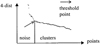 |
Fig. 1 Graph of distance of a point to its fourth-nearest neighbour (sorted in descending order) for a sample database in Ester et al. (1996). |
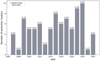 |
Fig. 2 Distribution of clusters and corresponding ϵ values (shown above each bar) per year. |
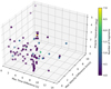 |
Fig. 3 Parameter characteristics of the first set of cluster candidates (i.e. before the study on the statistical significance). |
3 Results
3.1 First set of potential clusters
Applying the clustering algorithm to the entire dataset, we identified an initial set of 85 potential meteor clusters over a span of 16 years (2007–2022). It is worth mentioning at this point that this first set does not take into account the statistical significance tests, described in Sect. 3.3.
We examined the parameters of the identified clusters such as the number of fragments within a cluster, the maximum time separation between member fragments, their maximum velocity separation, and the maximum angular separation between their radiants. These characteristics are summarized in Figure 3. With the limited data available on confirmed clusters, we do not yet have well-defined upper limits for these quantities. Consequently, it is challenging to determine precise thresholds for the maximum permissible time between meteors, or the velocity and angular separation required to be considered a cluster.
3.2 Shower association
Having identified the potential candidates for clusters, the next question to answer was whether the clusters are real or whether they occur by chance. As a first step, we carried out a shower association test to determine which clusters are part of established meteor showers. In order to do so, we utilized the distance function, DN, defined by Valsecchi et al. (1999) to test the orbital similarity of meteoroid orbits with the shower orbits, based on their observed geocentric quantities. The computation was performed for every combination of meteors from our clusters and the known meteor showers (in the IAU Meteor Shower Databse3). We identified the minimum DN value for each meteor, which indicates the closest matching shower orbit. Thus, each meteor was associated with one shower based on this minimum DN value.
However, this association alone did not confirm that a meteor belongs to the identified shower. To determine if a given cluster is actually part of a shower, further analysis was required. Specifically, we took the median of the DN values for meteors within each cluster. According to Shober & Vaubaillon (2024), a DN criterion value of ~0.15 or less achieves a false-positive shower identification rate of less than 5%. Therefore, if the median DN value for a cluster is less than 0.15, we can confidently state that the cluster is part of the corresponding shower. Conversely, if the median DN exceeds 0.15, the cluster is likely not associated with the identified shower orbit and is therefore considered part of the sporadic meteors.
We found that 67 out of the 85 identified potential clusters are associated with some established showers. Figure 4 shows all cluster candidates, indicating their shower association. In particular, 67 cluster candidates are associated with seven established showers, with the majority (49 clusters) being in Geminids (GEM), ten in Perseids (PER), four in Orionids (ORI), one in Quadrantids (QUA), one in Comae Berenicids (COM), one in April Lyrids (LYR), and one in September ϵ-Perseids (SPE). Perseids, Geminids, and Quadrantids are among the most abundant known showers.
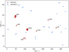 |
Fig. 4 Association of cluster candidates with known showers and the sporadic background. |
3.3 Statistical significance analysis
Knowing the shower associations of our identified cluster candidates, we proceeded to distinguish real clusters from chance occurrences. To do so, we compared the number of observed meteors in a cluster with a given time separation with the expected number of random appearances, N, which is given by the Poisson distribution (Porubčan et al. 2002):
 (2)
(2)
where n is the number of intervals (per hour), µ is the mean rate of meteors per interval, and x is the number of meteors in the cluster. More specifically, if all meteors in a cluster appeared within 2 s, then n = 1800. Consequently, µ was calculated as follows:
 (3)
(3)
where ZHR is the zenithal hourly rate.
For each shower, we took the maximum ZHR value that corresponds to the peak activity period of a meteor shower in order to obtain the upper limit of N. Similarly, for cluster candidates not associated with showers, we took the highest observed hourly rate of the sporadic meteors, HRspo = 11.6 (Dubietis & Arlt 2010). The ZHR values used in the computation of Ns are given in Table 1 and were taken from the International Meteor Organization4 (IMO) database.
It is important to highlight that the Poisson distribution was found to significantly underestimate the number of expected clusters (Koten et al. 2021). More precisely, Sampson (2007) determined from numerical analysis that the number of clusters appears to be three times more than what the Poisson model estimates. Therefore, a factor of three was added in our computations of N to account for this underestimation. In fact, conversely, our computations slightly overestimate the number of expected clusters, since we are using the maximum ZHR values (and not the ZHR at the time of the cluster), and the identified clusters were not necessarily observed during the peak activity of the showers or the sporadic background. These considerations make the method rather conservative.
The ZHR is defined for a field of view of a human naked eye, which, in turn, can be converted into a surveyed atmospheric area. Obviously, the number of observed meteors increases if this area increases. Stricto sensu, the analysis should take this effect into account by comparing the total area surveyed by the cameras involved in detecting a potential cluster to the area visible to the naked eye. Unfortunately, and as is discussed in further detail in Sect. 4.1, the database does not include any information regarding the camera parameters and pointing direction to estimate this effect. As a consequence, any cluster passing the statistical significance test described here must still be considered as a potential cluster.
The computed N values represent the number of expected clusters for one hour of observation by naked eye. Given that the observations were continuous, we needed to account for the total duration of the meteor showers for the cluster candidates that are associated with showers. Therefore, the N values were multiplied by the duration of the corresponding showers, yielding Ntot values. For each meteor shower, we took the ‘extreme’ window of time to ensure that N was maintained at the upper limit. The values used are given in Table 1. For the cluster candidates coming from the sporadic background, we used the temporal extent of the entire dataset (≈105 hours) for the duration. For each cluster we have identified, the expected number of such clusters (with the same number of meteors within the same period of time) Ntot is shown in Figure 5. We observe that, for the majority of clusters, the number of expected clusters is significantly high, Ntot > 1, indicating that these clusters could easily occur by chance. This validates the method of tuning epsilon to identify only the ten most promising clusters per year and not more because even among these, the majority are already being dismissed as random occurrences. Therefore, our focus shifts to clusters where the number of expected clusters is significantly below one. These clusters represent instances in which, given the specific number of fragments and time separation, we expect practically zero randomly occurring clusters. The fact that we detect a cluster in such a case implies that it is highly likely to be a real meteor cluster.
To restate our approach, we restricted our focus to ten or fewer clusters annually, utilized the maximum ZHR values to compute the expected cluster count, and set an extended observation period for the showers – all aimed at ensuring a ‘conservative’ method. By adopting these measures, which involve somewhat arbitrary choices, we are deliberately going for a cautious approach. This means we are potentially overestimating the likelihood that identified clusters may not be real. This cautious methodology allows for a margin of error in our selected parameters, thereby facilitating the identification of the most probable meteor clusters within the database. Of the initial 85 identified candidates, our statistical analysis results in 18 clusters with Ntot values that are sufficiently low to indicate that they are highly unlikely to have occurred by chance, given the method applied here.
Maximum ZHR value and total duration (in hours) of meteor showers used in the computation of the expected number of clusters.
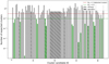 |
Fig. 5 For each detected cluster, this plot presents the expected number of random occurrences of such a cluster over the entire observation period. The clusters marked in green are considered potential candidates, while those in grey are dismissed as random occurrences. |
3.3.1 Monte Carlo simulation
To confirm the results of the adjusted Poisson distribution test, a Monte Carlo test for random occurrence of the meteor groups was prepared. For each cluster candidate, the ZHR number of random times of meteor occurrences within one hour were generated. It was then checked whether N meteors (the number of meteors in the cluster) occurred within Δt seconds (the duration of the cluster). Each step was repeated 100 000 times and the sum of positive occurrences was counted. All the accepted cluster candidates passed this test at the 3-sigma confidence level. For example, cluster candidate ID 9 (see Table 3), consisting of seven meteors within 7.78 s, belonging to the Geminid meteor shower, produces a random appearance in only 0.018% of all runs. The result for the ORI cluster candidate (ID 1) of four meteors observed in 6.048 s is 0.014%. On the other hand, a candidate consisting of four GEM meteors observed in 6.9 s was rejected as it randomly appears in 34.5% of all runs. Another GEM cluster of five meteors within 6.9 s occurs randomly in 3% of all the runs. The latter would be acceptable at the 2-sigma level but not at the 3-sigma level. Both of these clusters were equivalently dismissed as random occurrences based on the Poisson test. Some of the results are presented in Table 2. It can be concluded that the Monte Carlo test confirms the results of the adjusted Poisson test.
Monte Carlo test results for some cluster candidates.
Characteristics of the high-confidence meteor cluster candidates.
3.4 Potential high-confidence clusters
The characteristics of the potential high-confidence clusters are given in Table 3. Firstly, we rule out clusters 14 and 16 as being real meteor clusters due to the significant velocity separation, Δυɡ, between their member fragments, which indicates that it is implausible for these meteors to be physically related. This is because even a difference of a few kilometres per second can drastically change the orbital elements of the body, especially the semi-major axis. Checking the semi-major axes of the member meteors, we indeed find that they have a large range: 4–90 AU for cluster 14 and −2 to 17 AU for cluster 16 (where a negative semi-major axis represents a hyperbolic orbit with an eccentricity greater than one). However, it should be noted that SonotaCo’s reduction method and computation of orbital elements may cause a high uncertainty on the semi-major axis affecting the accuracy of these values. Nevertheless, the significant variation implies that the constituent meteors of these cluster candidates most likely do not follow the same orbit. Consequently, we are left with 16 candidates that can be considered high-confidence meteor clusters.
It is also important to note that after propagating the errors, we observe that some cluster candidates exhibit exceptionally high uncertainties. For instance, the angular separations for clusters ID 4, 7, 8, and 9 are particularly large, which affects our confidence in the reliability of these clusters. While we have maximized the use of the available data, this highlights the limitations of exploiting databases with high uncertainties and potential for improvement in future analysis with higher-precision data.
Overall, the analysis reveals a blend of various meteor showers alongside sporadic occurrences for the association of the high-confidence clusters. Specifically, six clusters belong to the Geminids, four to the Orionids, one to the Comae Berenicids, one to the April Lyrids, one to the September-epsilon Perseids, and three to the sporadic background (see Figure 6). A single cluster was previously identified during the September-epsilon Perseids by Koten et al. (2017), with no detection recorded for the other mentioned showers (Koten et al. 2021) or the sporadic background. Moreover, most of the previously detected meteor clusters have a cometary origin, whereas we observe that over one third of our detected clusters are in Geminids whose parent body is an active asteroid, 3200 Phaethon. This is interesting because while active asteroids also contain ice, they tend to have a higher proportion of rocky material compared to cometary meteoroids. Therefore, they tend to be less porous and more cohesive. Based on the detected clusters, initially thought to originate solely from comets and thus considered more prone to self-fragmentation, it now appears that meteoroids originating from asteroids may also exhibit this behavior.
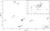 |
Fig. 6 High-confidence meteor cluster candidates. |
4 Discussion
4.1 Limitations of the method and choices
The main flaw in the described method is the absence of an estimate of the surveyed atmospheric area. The computation of such an area was last described in Vaubaillon et al. (2021), but dates back to the 1990s and has been improved several times (Koschack & Rendtel 1990; Koschny & Zender 2000; Gural & Jenniskens 2000; Ocaña et al. 2019). It involves knowledge of the camera’s field of view, but also its pointing direction above the local horizon. The equivalent surveyed area takes into account the magnitude loss as a function of air mass, physical distance, and meteor angular velocity. The larger the area surveyed by a network (or networks), the more likely it is to detect meteors per unit of time. This effect increases the number of expected clusters and could shorten the list of 16 identified statistically significant clusters. This is the reason why we call them ‘potential statistically significant clusters’. To account for this effect, the effective surveyed atmosphere area should be computed over time for each camera used requiring data on the field of view, pointing direction, and star limiting magnitude. Such information is routinely computed for astro-photometry and should be easily shareable by camera operators. Ideally, any cloud cover influencing the limiting magnitude and operational interruptions should also be considered to assess performance variations.
Currently, networks estimating meteoroid mass flux compute these parameters, but they may not be available for all networks. Unless an alternative method is developed to debias the cluster count, implementing this correction remains challenging. However, the IAU may require the addition of the camera field of view, pointing direction, and limiting magnitude (under clear sky conditions) to help in this matter. Such parameters are nearly constant over time and would allow us to put a lower limit on the real number of clusters, and hence help debias the observations.
4.2 Physical origin of cluster candidates
The physical origin of meteor clusters was thoroughly explored by Čapek et al. (2022). They considered fast rotation, collision, and thermal stress. The latter is considered as the most plausible, although an impact scenario cannot be totally ruled out. Considering a zero ejection velocity, dynamical analyses based on gravitational and non-gravitational forces acting on meteoroids have shown that the age of observed clusters range from a few hours to a few days at most (see Fig. 4 in Koten et al. 2017). The main reason is the differential non-gravitational forces acting on different sizes causing the fragment to disperse along the main orbit. However, the physical distance between the fragments is of the order of a few hundred kilometres at most. Here, the fragments of the potential statistically significant clusters detected both by CAMS and SonotaCo were potentially separated by a few thousand kilometres. A simple extrapolation from Koten et al. (2017) would conclude that their ages range from a few days to a few weeks. However, such considerations do not take into account any possible ejection velocity caused by thermal stress or collision. In the latter case, the physical survival of the fragments would be highly challenged, whereas for thermal stress their survival is evident. In order to produce a physical distance between the fragments of a few thousand kilometres, as would be the case if a cluster was detected, for example, from both Japan (SonotaCo) and California (CAMS), the ejection velocity would be evaluated from the total duration of the cluster. Considering a physical distance of 105 km and an age of 2 weeks, the estimated ejection velocity would be ~8 m s−1. But such a computation ignores the role of non-gravitational forces. Assuming that they account for only half of the physical distance of the fragments, the ejection velocity would be of a few metres per second only, which is compatible with thermal stresses.
It is worth pointing out that a significant fraction of cluster candidates originate from an asteroid (3200 Phaethon). The Geminids meteor shower is nearly as active as the Perseids, for which we find five fewer cluster candidates. As a first approximation, we expected fragile cometary meteoroids to self-fragment more often than less fragile asteroid dust, as Geminids are known for (Henych et al. 2024). However, our results show that clusters may occur regardless of the physical origin of the meteoroid. The low perihelion distance of the Geminids plays a crucial role in changing the meteoroid physical structure because of the high temperature difference they experience during their orbital revolution. For all these reasons, thermal stress appears to be the most likely physical process for the formation of meteor clusters (Čapek et al. 2022).
4.3 Towards a definition of a meteor cluster
As was previously mentioned, an official definition of a meteor cluster has not yet been established, with only eight reported clusters known to date. This study takes a step towards formulating a working definition by identifying twice as many potential cluster candidates as the currently confirmed ones. In this section, we discuss the features of these meteor clusters to help quantitatively characterize the phenomenon. However, our intention is not to set strict limits on any parameters, in order not to introduce any bias in future studies. Similarly, any strong limits, such as on the number of fragments may prove inadequate for future observations, potentially leading to false claims of meteor cluster detections when they are merely coincidental observations. Instead, we present some statistics of our set of 16 potential high-confidence meteor clusters and compare with the confirmed clusters where applicable.
To begin with, we examine the most critical parameter in the context of meteor clusters: the maximum time difference, Δt, between meteors within a cluster. Figure 7 (topmost subfigure) illustrates Δt for the 16 high-confidence clusters we identified, as well as for the eight confirmed clusters. Since there are no established thresholds for any parameter, we present the central tendency of the data by considering the 90th percentile. For the 16 clusters, the 90th percentile is 8.0 seconds and for the combined 24 clusters, it is 9.4 seconds. Here, we also know that the longest interval among the known meteor clusters was 11.3 seconds (Vaubaillon et al. 2023). We find that all Δt values lie within this range and are consistent with the conceptual definition of meteor clusters as short-duration events.
Furthermore, the middle subfigure in Figure 7 shows the velocity difference, Δυɡ, between the slowest and the fastest meteors within a cluster. In this case, a comparison between our high-confidence clusters and the eight confirmed clusters could not be performed as the information on velocities was not provided in all of the relevant literature. Consequently, among the 16 clusters considered, the 90th percentile value for Δυɡ was found to be 2.20 km/s, with roughly half of the clusters exhibiting a Δυɡ of less than 1 km/s. It should be noted that a robust computation of meteor velocities from video and photographic records is an extremely complex process. Egal et al. (2017) show that some data reduction pipelines introduce higher uncertainties on the velocity than claimed. The SonotaCo data reduction and orbit computation software is not publicly available, which prevents anyone from fully understanding the origin of the computed uncertainties. The velocity discrepancies are evident in Figure 8, in which the error bars are notably large in most cases. Such uncertainties are not optimal for our objective of defining the parameters of meteor clusters. This highlights the critical need for accurately determining orbital data using efficient pipelines.
The maximum angular separation, θ, between the geocentric radiants of the cluster fragments is illustrated in the bottom sub-figure of Figure 7. Similar to Δυɡ, data on the angular separation values for the eight detected clusters are absent in the literature; therefore, only the 16 that we identified are considered. For θ, 90% of the values lies below 3.89°. Similarly to Δυɡ, we observe extremely large uncertainties for some data points, making it challenging to precisely define representative values of angular separation.
Finally, the number of fragments within the high-confidence clusters ranges from four to seven, with the majority containing four meteors, which is relatively low compared to the confirmed clusters. Given that there are no defined limits for such characteristics of meteor clusters, it is challenging to ascertain what constitutes a low fragment count. Nevertheless, the clusters we have detected appear valid despite their lower fragment numbers. Thus, meteor clusters might not be as rare as only eight, but they also might not typically be as abundant as the majority of confirmed clusters. We believe that the previously detected clusters might have been detected primarily due to the higher intensity of their outbursts (i.e. higher number of fragments they contained) as well as their restricted physical extent, making them observable by a single camera. These elements strongly suggest potential observational bias for the detection of meteor clusters.
While we present the central tendencies of the cluster candidates, defining strict threshold values may overly constrain what can be classified as a meteor cluster. Instead, we propose a working definition based on the probability of chance occurrence rather than fixed parameter values. Specifically and on the basis of Fig. 5, if the expected number of random occurrences of such a cluster is less than 0.1, it can be considered a real cluster, as its occurrence is statistically unexpected. The relevant parameters, such as the number of meteors, time, velocity, and angular separation, can take any combination that results in this threshold being met.
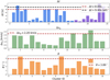 |
Fig. 7 Distributions of the parameters of high-confidence clusters, where Δt is the maximum time separation, Δυɡ is the maximum velocity separation between cluster fragments, and θ is the maximum angular separation between their geocentric radiants. The dashed red lines represent the 90 th percentiles of the dataset. In the topmost subplot, the blue bars represent the 16 clusters detected by us and the purple bars represent the eight confirmed clusters; the dashed black line represents the 90 th percentile for the two sets combined. |
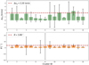 |
Fig. 8 Uncertainties associated with Δυɡ and θ. |
4.4 Future work and recommendations
The developed method can be applied to any meteor orbit database, provided it includes the parameters described in Sect. 2.2.1. Ideally, the camera’s field of view, pointing direction, and limited magnitude involved in the detection would also help to debias the observed number of clusters. We would also recommend that future reports of meteor clusters include the number of fragments, duration of the event, difference in velocity, and radiant separation, as it would help to define a cluster more precisely. In addition, we recommend that a detailed computation of the expected number of random occurrences of any future observed cluster is computed and published in order to confirm or revise our chosen threshold of 0.1. Finally, we recommend that the uncertainties of the angular separation and velocity are provided in order to strengthen the case of the detection of a meteor cluster.
Moreover, with the detection of more clusters than currently reported, and potential data from additional databases, the frequency of meteoroid self-fragmentation and its implications for the lifetime expectancy of meteoroids might be assessed. Current models of lifetime expectancy represent the collisional lifetime of meteoroids, calculated from the characteristics of the meteoroid, as well as the number and speed of projectile particles in interplanetary space that are capable of collisionally destroying the target meteoroid (Soja et al. 2019; Szalay et al. 2021). These collision models do not take into account the self-fragmentation lifetime of the meteoroids, which could potentially be a significant factor to consider.
5 Conclusions
After searching for meteor clusters in publicly available databases, we found 16 potential statistically significant clusters. This is twice as much as currently reported (at the time this article is written). Meteor clusters might be more frequent than currently reported. However, a fully debiasing analysis should take into account the atmospheric area surveyed by the cameras in order to definitively confirm the reality of the 16 potentially significant clusters. Unfortunately, such debias is not possible given the current parameters available in databases. We therefore recommend that anyone making a meteor orbit database includes the camera field of view, pointing direction, and limiting magnitude available for each detection. Any future meteor cluster detection claim should also provide a clear method of computing the expected number of cluster, to strengthen the case of a real cluster versus a random event. This number of expected events should be at most 0.1. Nevertheless, this study helps characterize the most common features of meteor clusters, which may in turn help to constrain a future official definition of a meteor cluster.
Acknowledgements
The authors are thankful to P. Shober who greatly helped with advice regarding the choice and use of the cluster algorithm. We are also grateful to the people maintaining the IAU meteor orbit database, which proved useful for this exploratory work.
References
- Bednář, J., Krauz, L., Páta, P., & Koten, P. 2023, MNRAS, 523, 2710 [Google Scholar]
- Capek, D., Koten, P., Spurný, P., & Shrbený, L. 2022, A&A, 666, A144 [NASA ADS] [CrossRef] [EDP Sciences] [Google Scholar]
- Dubietis, A., & Arlt, R. 2010, Earth Moon Planets, 106, 105 [Google Scholar]
- Ďurišová, S., Tóth, J., & Hajduková, M. 2023, Planet. Space Sci., 236, 105752 [Google Scholar]
- Egal, A., Gural, P. S., Vaubaillon, J., Colas, F., & Thuillot, W. 2017, Icarus, 294, 43 [NASA ADS] [CrossRef] [Google Scholar]
- Ester, M., Kriegel, H.-P., Sander, J., & Xu, X. 1996, in Second International Conference on Knowledge Discovery and Data Mining (KDD’96), Proceedings of a conference held August 2-4, 226 [Google Scholar]
- Gural, P. S., & Jenniskens, P. 2000, Earth Moon Planets, 82, 221 [Google Scholar]
- Hapgood, M. A., & Rothwell, P. 1981, Nature, 290, 384 [NASA ADS] [CrossRef] [Google Scholar]
- Henych, T., Borovička, J., Vojáček, V., & Spurný, P. 2024, A&A, 683, A229 [NASA ADS] [CrossRef] [EDP Sciences] [Google Scholar]
- Jenniskens, P., de Kleer, K., Vaubaillon, J., et al. 2008, Icarus, 196, 171 [NASA ADS] [CrossRef] [Google Scholar]
- Jenniskens, P., Gural, P. S., Dynneson, L., et al. 2011, Icarus, 216, 40 [NASA ADS] [CrossRef] [Google Scholar]
- Kinoshita, M., Maruyama, T., & Sagayama, T. 1999, Geophys. Res. Lett., 26, 41 [NASA ADS] [CrossRef] [Google Scholar]
- Koschack, R., & Rendtel, J. 1990, J. Int. Meteor Organiz., 18, 44 [Google Scholar]
- Koschny, D., & Zender, J. 2000, Earth Moon Planets, 82, 209 [Google Scholar]
- Koschny, D., Drolshagen, E., Drolshagen, S., et al. 2017, Planet. Space Sci., 143, 230 [NASA ADS] [CrossRef] [Google Scholar]
- Koten, P., Čapek, D., Spurný, P., et al. 2017, A&A, 600, A74 [Google Scholar]
- Koten, P., Rendtel, J., Shrbený, L., et al. 2019, in Meteoroids: Sources of Meteors on Earth and Beyond, eds. G. O. Ryabova, D. J. Asher, & M. J. CampbellBrown (Cambridge: Cambridge University Press), 90 [Google Scholar]
- Koten, P., Capek, D., Spurný, P., et al. 2021, A&A, 656, A98 [Google Scholar]
- Koten, P., Capek, D., Midtskogen, S., et al. 2024, A&A, 683, A5 [NASA ADS] [CrossRef] [EDP Sciences] [Google Scholar]
- Ocaña, F., Sánchez de Miguel, A., ORISON team, & Daedalus Project 2019, arXiv e-prints [arXiv:1911.10064] [Google Scholar]
- Piers, P. A., & Hawkes, R. L. 1993, J. Int. Meteor Organiz., 21, 168 [Google Scholar]
- Porubčan, V., Tóth, J., & Yano, H. 2002, Contrib. Astron. Observ. Skalnate Pleso, 32, 132 [Google Scholar]
- Sampson, R. D. 2007, JRASC, 101, 57 [NASA ADS] [Google Scholar]
- Shober, P. M., & Vaubaillon, J. 2024, A&A, 686, A130 [NASA ADS] [CrossRef] [EDP Sciences] [Google Scholar]
- Soja, R. H., Grün, E., Strub, P., et al. 2019, A&A, 628, A109 [NASA ADS] [CrossRef] [EDP Sciences] [Google Scholar]
- SonotaCo 2009, J. Int. Meteor Organiz., 37, 55 [Google Scholar]
- SonotaCo, Masuzawa, T., Sekiguchi, T., et al. 2021, J. Int. Meteor Organiz., 49, 64 [Google Scholar]
- Sugar, G., Moorhead, A., Brown, P., & Cooke, W. 2017, MAPS, 52, 1048 [Google Scholar]
- Szalay, J. R., Pokorný, P., Malaspina, D. M., et al. 2021, Planet. Sci.-J., 2, 185 [Google Scholar]
- Valsecchi, G. B., Jopek, T. J., & Froeschle, C. 1999, MNRAS, 304, 743 [NASA ADS] [CrossRef] [Google Scholar]
- Vaubaillon, J., Rietze, A., & Zilkova, D. 2021, MNRAS, 9999 [Google Scholar]
- Vaubaillon, J., Loir, C., Ciocan, C., et al. 2023, A&A, 670, A86 [NASA ADS] [CrossRef] [EDP Sciences] [Google Scholar]
- Watanabe, J.-I., Sekiguchi, T., Shikura, M., Naito, S., & Abe, S. 2002, PASJ, 54, L23 [NASA ADS] [CrossRef] [Google Scholar]
- Watanabe, J.-I., Tabe, I., Hasegawa, H., et al. 2003, PASJ, 55, L23 [NASA ADS] [CrossRef] [Google Scholar]
- Williams, I. P., Jopek, T. J., Rudawska, R., Tóth, J., & Kornoš, L. 2019, in Meteoroids: Sources of Meteors on Earth and Beyond, eds. G. O. Ryabova, D. J. Asher, & M. J. Campbell-Brown (Cambridge: Cambridge University Press), 210 [Google Scholar]
https://iaumeteordatacenter.org, accessed in Jan. 2024.
Documentation on sklearn.cluster.DBSCAN (accessed in February 2024).
IAU MDC established meteor showers list (accessed in April 2024).
IMO 2024 Meteor Shower Calendar (accessed in May 2024).
All Tables
Maximum ZHR value and total duration (in hours) of meteor showers used in the computation of the expected number of clusters.
All Figures
|
Fig. 1 Graph of distance of a point to its fourth-nearest neighbour (sorted in descending order) for a sample database in Ester et al. (1996). |
| In the text | |
|
Fig. 2 Distribution of clusters and corresponding ϵ values (shown above each bar) per year. |
| In the text | |
|
Fig. 3 Parameter characteristics of the first set of cluster candidates (i.e. before the study on the statistical significance). |
| In the text | |
|
Fig. 4 Association of cluster candidates with known showers and the sporadic background. |
| In the text | |
|
Fig. 5 For each detected cluster, this plot presents the expected number of random occurrences of such a cluster over the entire observation period. The clusters marked in green are considered potential candidates, while those in grey are dismissed as random occurrences. |
| In the text | |
|
Fig. 6 High-confidence meteor cluster candidates. |
| In the text | |
|
Fig. 7 Distributions of the parameters of high-confidence clusters, where Δt is the maximum time separation, Δυɡ is the maximum velocity separation between cluster fragments, and θ is the maximum angular separation between their geocentric radiants. The dashed red lines represent the 90 th percentiles of the dataset. In the topmost subplot, the blue bars represent the 16 clusters detected by us and the purple bars represent the eight confirmed clusters; the dashed black line represents the 90 th percentile for the two sets combined. |
| In the text | |
|
Fig. 8 Uncertainties associated with Δυɡ and θ. |
| In the text | |
Current usage metrics show cumulative count of Article Views (full-text article views including HTML views, PDF and ePub downloads, according to the available data) and Abstracts Views on Vision4Press platform.
Data correspond to usage on the plateform after 2015. The current usage metrics is available 48-96 hours after online publication and is updated daily on week days.
Initial download of the metrics may take a while.