| Issue |
A&A
Volume 696, April 2025
|
|
|---|---|---|
| Article Number | A191 | |
| Number of page(s) | 16 | |
| Section | Numerical methods and codes | |
| DOI | https://doi.org/10.1051/0004-6361/202452117 | |
| Published online | 25 April 2025 | |
Coupling particle-in-cell and magnetohydrodynamics methods for realistic solar flare models
1
Rosseland Centre for Solar Physics, University of Oslo,
PO Box 1029 Blindern,
0315
Oslo, Norway
2
Institute of Theoretical Astrophysics, University of Oslo,
PO Box 1029 Blindern,
0315
Oslo, Norway
3
Niels Bohr Institute, University of Copenhagen,
Jagtvej 155A,
2200
Copenhagen, Denmark
★ Corresponding author; This email address is being protected from spambots. You need JavaScript enabled to view it.
Received:
5
September
2024
Accepted:
25
March
2025
Abstract
Context. Simulating solar flares requires capturing both large-scale magnetohydrodynamic (MHD) evolution and small-scale kinetic processes near reconnection sites. Bridging these scales has been a significant computational challenge.
Aims. This study introduces a Particle-In-Cell (PIC) solver integrated within the DISPATCH framework, facilitating seamless embedding within MHD simulations. This development aims to enable self-consistent multi-scale solar flare simulations.
Methods. Our PIC solver, inspired by the PhotonPlasma code, addresses the Vlasov-Maxwell equations in collisionless plasma. We validate its accuracy through fundamental plasma tests – including plasma oscillations, two-stream instability, and current sheet reconnection. To make kinetic simulations computationally feasible, we employ physical adjustment of constants (PAC), modifying the speed of light, elementary charge, and electron mass to shift plasma scales. Additionally, we implement and validate a coupling strategy that enables smooth transitions between kinetic and fluid regimes.
Results. The PIC solver successfully recovers expected plasma dynamics and electromagnetic field behaviour. Our analysis highlights the effects of PAC on reconnection dynamics, underscoring the importance of transparent and well-documented scaling choices. Test cases involving propagating waves across PIC-MHD interfaces confirm the robustness of our coupling approach.
Conclusions. The integration of the PIC solver into the DISPATCH framework makes it possible to run self-consistent, multiscale solar flare simulations. Our approach provides a computationally efficient foundation for investigating reconnection physics in large-scale astrophysical plasmas.
Key words: magnetohydrodynamics (MHD) / plasmas / methods: numerical / Sun: atmosphere / Sun: flares
© The Authors 2025
 Open Access article, published by EDP Sciences, under the terms of the Creative Commons Attribution License (https://creativecommons.org/licenses/by/4.0), which permits unrestricted use, distribution, and reproduction in any medium, provided the original work is properly cited.
This article is published in open access under the Subscribe to Open model. This email address is being protected from spambots. You need JavaScript enabled to view it. to support open access publication.
1 Introduction
Simulating solar flares, encompassing both the large-scale evolution of magnetic structures and the fine-scale physics of current sheets forming during magnetic reconnection, remains a significant computational challenge. According to recent work (Guo et al. 2024), no existing computational tool fully captures both the global dynamics of solar flares and the intricate kinetic processes occurring in reconnection regions.
Solar flares are generally understood to result from the sudden release of magnetic energy via reconnection (Zharkova et al. 2011). In these regions, some particles are accelerated to non-thermal, relativistic speeds, exchanging energy with the surrounding plasma. The presence of these high-energy particles induces non-local effects that influence plasma behaviour on macroscopic scales, which in turn affects the dynamics of reconnection on smaller scales. Capturing this complex interplay between kinetic and fluid scales is crucial for understanding the initiation and development of solar flares.
Kinetic approaches, particularly the Particle-In-Cell (PIC) method (Liu et al. 2022; Klion et al. 2023; Selvi et al. 2023), have been extensively applied to study reconnection at microscales. However, due to computational constraints, these studies often rely on simplified configurations, such as the 2D Harris sheet model (Harris 1962), and are impractical for the vast spatial scales of real-world solar flares. Although hybrid approaches that combine Magnetohydrodynamics (MHD) and PIC methods have been explored (Baumann et al. 2013; Daldorff et al. 2014), significant challenges remain in achieving more cost-effective multi-scale hybrid models.
The work by Baumann et al. (2013) indirectly demonstrated the potential for significant cost reductions, in that only a small fraction of the domain covered by the PIC solver in that experiment actually developed significant non-thermal particle distributions, suggesting that a multi-physics enabled setup could employ an inexpensive MHD method in much of the volume, provided it could be smoothly coupled to a PIC method covering the small fraction of the volume where significant particle acceleration actually is taking place.
A closely related obstacle in solar flare modelling is the extreme separation of scales: macroscopic structures span megametres, while kinetic processes occur at centimetres or smaller scales. Resolving both within a single computational framework is infeasible with uniform resolution. A promising strategy to overcome this limitation is adaptive mesh refinement (AMR), where high resolution is applied only in regions where kinetic effects are significant. However, even with AMR, the separation between kinetic and global scales remains computationally prohibitive.
To further bridge this scale gap, we employ a well- established technique in which fundamental physical constants such as the speed of light, elementary charge, and electron mass are adjusted to shift kinetic scales to more computationally feasible regimes. We chose to refer to this technique as physical adjustment of constants (PAC). While the technique has been widely used in plasma simulations (Hesse et al. 1999; Baumann et al. 2013; Liu et al. 2022; Hesse et al. 2018; Malakit et al. 2010), our implementation emphasizes flexibility and transparency, allowing for consistent tuning of scale ratios to suit different physical setups. By combining AMR with PAC, we aim to resolve both large-scale dynamics and kinetic processes within the same simulation, significantly reducing computational costs while maintaining physical realism.
Handling the wide range of temporal and spatial scales in solar flare simulations, while maintaining computational performance, is a significant challenge. Developing a sophisticated multi-scale, multi-physics solver from scratch would be daunting. Fortunately, the DISPATCH framework (Nordlund et al. 2018) provides a robust foundation for handling the scales required to simulate solar flares and already has AMR capabilities. DISPATCH organizes the simulation domain into ‘patches’, each updated semi-autonomously. This localized data management enables ‘multi-physics’ simulations, where different patches or groups of patches use different solvers. DISPATCH has already proven capable of modelling complex, multi-scale environments, such as the entire solar convection zone (Popovas et al. 2022), and with the hybrid MHD/PIC method introduced here, we extend the DISPATCH framework to also allow multi-physics simulations.
In this paper, we present the development of a hybrid PIC- MHD setup within DISPATCH. We have integrated a PIC solver inspired by the PhotonPlasma code (Haugbølle et al. 2013) and detail the modifications made to ensure compatibility within the DISPATCH architecture. We then describe our coupling strategy and assess the functionality of the PIC-MHD integration. Through this work, we aim to provide a computationally efficient framework that bridges the gap between large-scale flare dynamics and the detailed kinetic processes occurring in reconnection regions, contributing to a more comprehensive understanding of solar flare mechanisms.
2 Methods
2.1 Governing equations
The PIC solver implemented in this study solves the Vlasov- Maxwell system of equations.
To enhance reproducibility and clarity, we outline only the most important equations here. For an exhaustive description, readers are referred to the original description of the PhotonPlasma code (Haugbølle et al. 2013). In our notation, we use bold letters to indicate vectors. The Vlasov-Maxwell system is represented as follows:
 (1)
(1)
Here, f is the distribution function, which is a function of time, velocity (u), and space (x). s denotes particle species (e.g. electrons, protons),  the relativistic Lorentz factor and C the collision operator. Finally, E and B are the electric and magnetic fields respectively. For this study, we focus on the collisionless regime, setting C = 0.
The electric and magnetic fields’ evolution follows the Maxwell equations:
 (2)
(2)
Constants used in the Maxwell-Lorentz equations for systemagnostic formulation.
 (3)
(3)
 (4)
(4)
 (5)
(5)
where J and ρc represent the current density and charge density, respectively.
The constants kF kE, and kB ensure the equations’ consistency across different unit systems, as detailed by Carron (2015). We show the values corresponding to SI, CGS, and HL units in Table 1. The use of this unit-agnostic formulation is commented on in Section 2.3.3
The PIC solver approximates the Vlasov Equation (Eq. (1)) by sampling the phase space with ‘macro particles’, each representing a collection of real particles, as discussed in works such as Birdsall & Langdon (1991) and Lapenta et al. (2006). Macro particles are assigned a weight that represents the number of real particles they sample. The macro particles are then treated as individual particles, with their velocities influenced by the Lorentz force:
 (6)
(6)
and their positions evolve as per:
 (7)
(7)
Here up and xp are the velocity and position of each macro particle. qs and ms are the charge and mass of the particle species.
Interpolating electric and magnetic fields to macro particle positions requires assigning specific shapes to these particles, affecting field interpolation. Following PhotonPlasma’s methodology, we have implemented various shape functions, including nearest-grid-point (NGP), cloud-in-cell (CIC), triangular- shaped-cloud (TSC), and piecewise-cubic-spline (PCS), noting that NGP can introduce instabilities (Birdsall & Langdon 1991; Smets et al. 2021). We use ‘CIC’ interpolation and 2nd order derivatives as the default in our solver.
Determining properties such as charge density from particle distributions uses similar shape functions, and we refer to this as ‘particle deposition’ in this article. The interpolation and deposition shape functions can be defined independently as simulation input parameters.
2.2 MHD solvers in DISPATCH
The DISPATCH framework has a variety of MHD type solvers implemented. During our development we have used both the Riemann and Bifrost solvers available in the framework. The Riemann solver uses the RAMSES (Teyssier 2002) scheme. It is an HLLD-type (Miyoshi & Kusano 2005) Riemann solver and uses an extension to the HLLD to include the induction equation in a constrained transport formulation (Fromang et al. 2006). The Bifrost code (Gudiksen et al. 2011) solves the resistive MHD equation with ‘hyper-resistivity’. It has been developed with the main focus of modelling the dynamics in the solar atmosphere. We use the Bifrost solver as the ‘background’ MHD solver when running embedded PIC simulations unless otherwise stated.
2.3 Transparent scaling
2.3.1 Unit scaling
Simulation parameter scaling is critical for ensuring both stability and optimized simulation performance. Although frequently mentioned in scientific literature, the detailed methodologies for scaling are often not fully elaborated, posing challenges to reproducibility. In response, we aim to clearly outline the scaling techniques employed in our study.
Within the DISPATCH framework, we have incorporated a scaling module to handle scaling for SI, CGS, and HL unit systems. This module relies on three primary parameters for scaling: mass density, length, and time. The scaling of all subsequent units stems from these foundational parameters.
Often, variables of interest such as the proton mass, the elementary charge, and the speed of light, are set to 1 in code units. Along with this, pressure, density, and field strength are usually given in code units (normalized to simplify calculations) as well, making it difficult to recover the ‘real’ physical units. For ease of physical interpretation and to ensure that input parameters remain intuitive, we have based all scaling on real physical units. As such, the code is designed to accept input parameters in familiar terms, including common length scales, magnetic field strengths, number densities, and temperatures.
2.3.2 Physical adjustment of constants
A common practice in PIC simulations is the adjustment of physical constants to change time and length scales to make simulations computationally feasible. We will refer to this as ‘physical adjustment of constants’ (PAC), meaning the intentional adjustment of physical constants in real units. Although critical for simulation fine-tuning, this process is frequently glossed over in the literature, leaving a gap in understanding regarding the specific adjustments made. We aim to demystify this aspect by ensuring complete transparency in our scaling process.
In our simulations, we permit the modification of three key constants: the speed of light, electron mass, and elementary charge. The modification of the speed of light is facilitated through changes to the vacuum permeability, μ0, or vacuum permittivity, ϵ0. Specifically, in CGS and HL units where μ0 is dimensionless, speed of light adjustments are achieved by modifying ϵ0.
2.3.3 Unit-agnostic equations
The Vlasov-Maxwell system of equations varies depending on the unit system used. The unit system is often implicit, with equations written in ‘natural units’ where constants like 4π are omitted. Gaussian and Heaviside-Lorentz (HL) are examples of ‘natural units’ and are often both referred to as CGS. Although units appear identical in Gaussian and HL units, their actual values differ. For instance, a magnetic field strength of 50G in Gaussian units corresponds to approximately 14.1G in HL units, differing by a factor  . While readers may often be able to deduce the underlying unit system, even when it is not explicitly stated, this can sometimes be problematic, making it challenging to reproduce results if the exact unit system is not specified.
PAC also alters the equations. When ambiguous PAC is combined with an ambiguous unit system, it may present a complex puzzle for the reader to solve.
We write all equations in a unit-agnostic form to assist the reader. Constants are included in the equations, and these constants vary depending on the unit system and the PAC used, as shown in Table 1. This approach allows us to use the same equations in both ‘real’ and code units, simplifying implementation and improving the clarity of presentation, as well as of the code.
2.4 Numerical approach
2.4.1 DISPATCH
A fundamental understanding of the DISPATCH framework is essential to explain some of the decisions made when integrating the PIC code. We summarize the key aspects relevant to our integration here, while a detailed description of DISPATCH can be found in Nordlund et al. (2018).
DISPATCH organizes the simulation domain into distinct sections called ‘patches’, which are updated semi-autonomously. These patches interact with neighbouring patches primarily by exchanging ghost zone information. This architecture offers substantial benefits, including the ability for each patch to evolve with its own time step. This feature significantly improves computational efficiency by allowing the simultaneous resolution of different timescales within a single experiment.
Patches typically range in size from 163 to 323 cells, although the user can customize this size as needed for the specific problem. Patch sizes are selected to fit within the CPU cache, maximizing memory access efficiency and speed. In simulations, all patches contain the same number of cells, but their physical size may vary when adaptive mesh refinement (AMR) is enabled, allowing for finer resolution in regions of interest.
A key feature of DISPATCH is its local time stepping approach, where each patch determines its time step based on local conditions, such as the Courant condition. This results in asynchronous time updates between patches, meaning neighbouring patches may advance at different rates. To ensure consistency, patches rely on ghost zones for boundary information exchange. When a patch requires data from a neighbour at a different time step, temporal interpolation is applied to fill its ghost zones. Multiple time slices – typically five – of each patch’s data are stored, enabling accurate interpolation over time.
In distributed simulations using MPI, patches are distributed across multiple MPI processes. Patches at subdomain boundaries are flagged as ‘boundary’ patches (computed on their home MPI rank) or ‘virtual’ patches (replicated on neighbouring MPI ranks). ‘Boundary’ patches send updated data to neighbouring ranks, allowing ‘virtual’ patches to maintain up-to-date information. This ensures the most recent information is accessible from neighbour patches on all MPI ranks.
The ghost zone interpolation and MPI communication are handled independently within the framework, separate from the solvers themselves. This modular design simplifies the implementation of new solvers within DISPATCH.
The framework’s emphasis on localized data management limits the applicability of global convergence schemes, such as implicit methods. We therefore initially chose a fully explicit PIC solver as this better fits within DISPATCH’s decentralized data-handling paradigm. However, we have also implemented the semi-implicit field solver from the PhotonPlasma code which evolves locally within each patch. While this in principle requires globally implicit solutions, using a patch-local implicit formulation works remarkably well, and we found this to be more stable when embedding PIC in MHD.
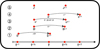 |
Fig. 1 Time staggering of the explicit PIC solver in DISPATCH, illustrating the integration order. The electric field is staggered by a full time step, Δt in the past. Magnetic field, particle velocities, and current density are staggered backwards by 0.5Δt. Particle position is centred in time. |
2.4.2 Discretization
We have implemented both a fully explicit and a semi-implicit scheme. We focus our description here on the explicit scheme and refer readers interested in the semi-implicit scheme to Haugbølle et al. (2013).
For the numerical stability and reliability of our explicit computational scheme, we incorporate a time-staggering method akin to the leap-frog integration technique, as visually represented in Figure 1. The leap-frog scheme (Feynman et al. 1965, section 9.6) or (Birdsall & Langdon 1991, p. 56) is renowned for its ability to maintain stability during oscillatory motion – a common occurrence within PIC simulations. The electric field is staggered by a full time step, Δt in the past. Magnetic field, particle velocities, and current density are staggered backwards by 0.5Δt. Particle position is centred in time. For the semi-implicit scheme, the magnetic fields are staggered a full time step in the past, such that it is temporally co-located with the electric field.
Spatially, we stagger mesh variables in accordance with a Yee lattice setup Kane Yee (1966). This spatial organization involves positioning magnetic fields on the cell faces, electric fields and current densities along cell edges, and charge density in corners. For Riemann-type MHD solvers, mass density, momentum, and energy metrics are centred within each cell as shown in Figure 2. For the Bifrost solver, momentum is downward staggered, similar to the magnetic field. This arrangement of variables in time and space minimizes the interpolation needed, thereby improving the simulation’s computational efficiency and accuracy.
In our simulation, both electric and magnetic fields are interpolated from the mesh to each particle’s position. Interpolating fields to particle positions involves considerations of both time and space. As outlined in Figure 1, the magnetic field requires time interpolation between the time step i, and time step i + 1. With varying time steps, this introduces the potential for this time interpolation to become desynchronized. Within the DISPATCH framework, each patch dynamically sets its time step based on the local maximum velocity to comply with the Courant condition (Courant et al. 1928). This approach is applied to all patches in the simulation, including the PIC solver patches. Because of the PIC solver’s focus on electromagnetic phenomena and the need to accurately simulate the propagation of electromagnetic waves at the speed of light, the ‘maximum velocity’ in PIC patches defaults to the speed of light. This condition results in uniform time steps across these patches. Consequently, time interpolation for the magnetic field is simplified to averaging B1 and B1+1, as outlined in Figure 1.
Spatially, after addressing time interpolation, fields are then interpolated to the exact locations of particles. This spatial interpolation relies on the shape functions introduced in Section 2.1.
Particle deposition into current density, mass density, and other mesh variables happens after the particles have been updated, as described in Sections 2.4.5 and 2.4.6. This process ensures that changes in particle distribution are accurately reflected in the mesh. Consequently, electromagnetic field calculations can incorporate the most current state of the plasma. We allow the shape function for deposition to differ from the one used for interpolation, but as default the shape functions are identical.
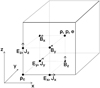 |
Fig. 2 Spatial staggering of mesh variables on a Yee lattice. Magnetic fields are located on the cell faces, electric fields, and current densities on the edges, with mass density, momentum, and energy centred within each cell. Charge density is uniquely staggered to the lower corner of each cell. |
2.4.3 Solving Maxwell’s equations
For the explicit scheme, the update process begins by advancing Ei to Ei+1 (Figure 1), using Eq. (2). This calculation uses the magnetic field, Bi, alongside the current density, Ji. The magnetic field is then updated in line with Eq. (3), using the just-updated electric field. For the semi-implicit method, the magnetic field is first updated with an implicit step and then the electric field is updated with an explicit step using an average between the new and old magnetic field values.
Inside patches, the Yee arrangement ensures that the magnetic field evolution is div(B)-conserving, which however still allows round-off and truncation errors to accumulate over time. Moreover, the time-interpolation of values in the ghost zones does not conserve div(B) exactly. To keep the magnetic field divergence-free to within numerical precision, the DISPATCH framework uses a div(B)-cleaner, which corrects B with
 (8)
(8)
where ΦB is the solution of
 (9)
(9)
Note that, since errors are entirely local, there is no need to solve a global Poisson equation; the solution adopts Φ = 0 as a boundary condition in the ghost zones.
A similar cleaning strategy is applied to the electric field to ensure it meets the requirements of Eq. (5). The cleaning process starts by calculating the divergence error, ϵ, through the calculation of the electric field’s divergence, from which the charge density is then subtracted:
 (10)
(10)
A subsequent Poisson solution step produces Φϵ from
 (11)
(11)
after which the electric field is updated to a ‘cleaned’ state with
 (12)
(12)
The implementation allows users to decide the frequency of the cleaning steps and whether to use them at all.
2.4.4 Particle movement
Next in the update cycle, particle velocities are updated, affecting both particles in the ‘inner’ domain and those within the ghost zones. As highlighted earlier, electric and magnetic fields are interpolated to each particle’s position to enable accurate velocity updates.
Velocity updates are governed by the Lorentz force Equation (Eq. (6)). Ripperda et al. (2018) compares several different explicit approaches to implement this numerically. We have chosen to use the Vay particle pusher algorithm (Vay 2008) due to its ability to correctly ‘cancel’ field contributions when both electric and magnetic fields act on particles. Following the velocity updates, we calculate the relativistic kinetic energy for each macro particle. Then, their positions are updated according to Eq. (7).
With updated positions and velocities, the simulation is prepared for the next and final phase - the deposition of particle data back to the mesh. In this stage, the current density is computed from particle positions and velocities, which is essential for updating the electric field in the next time step. Additionally, other mesh variables, such as mass density and bulk momentum, are computed from particle deposition.
2.4.5 Current density calculation
Accurate current density calculation is essential for maintaining PIC simulation accuracy. PIC codes often employ a ‘chargeconserving’ method to ensure charge continuity during simulations. For example, the PhotonPlasma code uses an extension of the charge-conserving method developed by Esirkepov (2001). This method involves calculating the divergence of the current density by examining how the deposition weights for each macro particle change between time steps. After determining the divergence, the current density is computed through a prefix sum operation.
In DISPATCH, using such a prefix sum operation would require inter-patch communication to align ghost values with neighbouring patches. The current communication scheme does not directly allow this, and we, therefore, opted for a simpler and more direct current density calculation:
 (13)
(13)
where W(xp−xc) represents the deposition weight function, wi the weight of the macro particle, ui the velocity of the macro particle, and qs the charge of the particle species. This method calculates current density directly from the macro particles’ properties.
Although not precisely charge-conserving at the level of each macro particle’s individual contribution, the method is nevertheless on average charge-conserving, with errors expected mainly on cell scales, where E-field cleaning (Eqs. (11)-(12)) can easily take care of making the electric field consistent with the actual charge distribution.
2.4.6 Mesh deposition
The deposition of mass density, bulk velocity, and pressure occurs in the same step as the calculation of current density. Mass density and bulk velocity are summed in a manner similar to current density. From these, the momentum is computed, which is required by the MHD solvers.
To estimate pressure, we adopt an isotropic formulation that aligns with the pressure assumptions in our MHD solver. While this choice does not perfectly capture all physical conditions, it ensures a smooth and consistent transition between the PIC and MHD regions. By maintaining compatibility with the MHD solver’s pressure treatment, we reduce potential discontinuities at the interface.
We employ two methods to estimate pressure. The first and simplest approach computes the isotropic pressure for each species, s, as
 (14)
(14)
After summing over all particles, we subtract the bulk velocity contribution to obtain the final pressure:
 (15)
(15)
following the approach of Daldorff et al. (2014), where ux, uy, and uz are the bulk velocity flows. This method allows pressure to be computed efficiently during the deposition of other mesh variables. However, it tends to underestimate pressure, particularly in regions with high bulk flow.
The second approach, which is computationally more demanding but provides improved accuracy, is performed after computing the bulk velocity. Here, pressure is determined as
 (16)
(16)
This method is the default due to its better accuracy. The final pressure is obtained by summing over all species. Pressure is then converted to internal energy using the ideal equation of state,  , where we assume γ = 5/3.
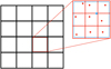 |
Fig. 3 Illustration of particle sampling in a 2D setup with 10 particles per cell. Each cell is divided into |

2.4.7 Initial condition sampling
Initial particle sampling in our simulation relies on MHD mesh variables, including mass density, momentum, and internal energy. To distribute particles evenly at the start, we segment each cell into a predefined number of sectors. The number of sectors, nsec, varies with the dimensionality of the simulation:
 (17)
(17)
where D, is the dimensionality. In a 2D setup with 10 particles per cell, nsec = 3, dividing each cell into 3 × 3 = 9 sectors. One particle is placed randomly within each sector, with any additional particles randomly located within the entire cell, as depicted in Figure 3.
Once particle positions are set, their velocities are sampled from a Maxwellian distribution. The initial temperature for this distribution is either provided directly or derived from the internal or total energy, depending on the initial conditions. Additionally, we incorporate bulk and current velocities into the velocity assignment for particles, similar to the approach described by Daldorff et al. (2014):
 (18)
(18)
 (19)
(19)
where ubulk represents the bulk velocity, J is the current density derived from  , ρ is the mass density from grid, and mi, qi, me, qe are the masses and charges of protons and electrons, respectively.
This initial velocity assignment is based on two key assumptions: (1) the initial velocities are non-relativistic and thermal, and (2) the bulk flow of each particle species essentially follows Hall-MHD principles. We emphasize that this assumption remains valid even when the underlying MHD model is ideal MHD and not explicitly Hall-MHD. The Hall-MHD effects are implicitly incorporated through the calculation and imposition of the bulk velocity on each particle species, even though the governing equations are those of ideal MHD.
Each particle’s final velocity combines the thermal velocity, sampled from a Maxwellian distribution, with the bulk velocity computed from Equations (18) and (19), resulting in a drifting Maxwellian distribution. This prescription is valid as long as the particle speeds are non-relativistic. As the intended use of this PIC solver is within MHD simulations, particles are always initialized from an ‘MHD region’ where the underlying assumption of non-relativistic velocities applies. Thus, this assumption is consistently valid for initialization in our use cases.
2.4.8 Resampling
Within the inner domain of a patch, particles are free to move between cells. Over time, this freedom can lead to significant discrepancies in the number of particles per cell, with some cells becoming overcrowded and others underpopulated. Similar discrepancies can develop at the patch level. To maintain a roughly constant number of particles per cell and ensure workload balance across patches, we’ve implemented a resampling strategy that involves ‘splitting’ particles in underpopulated cells and ‘merging’ particles in overcrowded ones.
Splitting, or up-sampling, involves dividing the heaviest particle in a cell into two particles, each retaining the original velocity and carrying half the weight. To prevent creating identical particles, a slight positional offset is introduced. This offset is randomly determined in each dimension from a Maxwell distribution with σ = 0.1 cells, with one particle receiving half the offset subtracted and the other half added. This process can be repeated until the desired number of particles per cell is achieved.
Merging, or down-sampling, is more complex, as it must account for the conservation of mass, energy, and momentum. Drawing on strategies discussed by Muraviev et al. (2021), we’ve adopted the ‘levelling’ approach from their work and introduced a ‘close-phase’ strategy. For the latter, we evaluate particle velocities within the same cell using the Euclidean distance metric, merging the two particles closest in velocity space into one – conserving momentum to machine precision. However, this process does not strictly conserve energy. To mitigate this, the new particle’s energy is compared to the total energy of the original pair. If the energy discrepancy falls within an acceptable tolerance, the merge is finalized; otherwise, the particle is discarded. This process repeats until the target particle count is achieved or all potential merges are explored without success due to excessive energy differences. The default down-sampling approach is the close-phase strategy.
Resampling primarily balances computational load across patches and only occurs when a patch’s total particle count deviates by more than ±20% from the target number. Similarly, at the cell level, resampling is triggered only if the particle count in a cell exceeds ±20% of the target particle number per cell.
The frequency and activation of resampling are customizable, allowing users flexibility in managing simulation dynamics. Both particle splitting and merging affect particle deposition onto the mesh, slightly disrupting strict charge conservation within the solver. However, our findings indicate that this effect remains minimal when resampling is applied selectively to areas with particularly high or low particle counts. In Section 4.3, we demonstrate that even with resampling every 100 updates, the reconnection rate is only slightly affected.
More sophisticated merging strategies, such as those described by Chen et al. (2023), aim to merge multiple particles while preserving higher-order moments of the distribution function. While these approaches improve accuracy, they also introduce additional computational overhead. Given our focus on maintaining computational efficiency, we have opted for a simpler merging strategy that balances accuracy with performance, ensuring minimal disruption to the simulation while keeping resampling computationally cheap.
2.5 Particle communication between patches
Particle communication between patches ensures continuity across the computational domain. This process is handled through the use of export buffers and ghost zones, allowing particles to move seamlessly between neighbouring patches.
Each patch establishes an export buffer in each neighbouring direction to facilitate particle exchange. This setup results in two buffers in one-dimensional simulations, eight buffers in two dimensions, and 26 buffers in three dimensions. These buffers also store multiple timeslots, enabling the proper handling of asynchronous updates between patches.
After each update, particles near the edge of a patch’s inner region are placed into the corresponding export buffer, marking them for transfer to neighbouring patches. Before updating, a patch will inspect the export buffers from all its neighbours and copy any particles into its ghost buffer, where they are stored until the next update.
During the update process, the patch updates both its inner region and the particles in the ghost buffer. If any particles move from the ghost buffer region into the inner region of the patch, they are copied over and now ‘belong’ to the patch. Conversely, any particles that leave the inner region are immediately destroyed, as the neighbouring patch will have already copied the particle into its ghost buffer and will take ownership of it when it moves into its inner region.
Field quantities, like charge density and current, are communicated separately by the DISPATCH framework, efficiently decoupling particle and mesh communication.
2.6 Optimization
Optimization is essential to develop a comprehensive and realistic multi-scale solar flare model. We’ve introduced several optimizations to boost the performance of our simulation framework, preparing for future enhancements.
Our simulation follows a Particle-in-Patch (PIP) approach, which aligns with DISPATCH’s strategy of updating entire patches rather than individual cells. This method optimizes cache usage and enables effective vectorization of computations. In our PIC solver, each patch hosts several arrays of particle information, facilitating vectorization. Although these arrays exceed cache capacity and are less ideal for traditional computing, their structure is well-suited for GPU execution. GPU acceleration remains a key development goal, given its potential to significantly enhance simulation performance.
A fundamental part of our optimization strategy involves sorting particles to improve memory access patterns. Placing spatially proximate particles adjacent in memory significantly increases the efficiency of interpolation and deposition operations. We store particle positions in two arrays: an integer array for cell location and a floating array for position within the cell. This dual-array setup simplifies sorting, allowing for integerbased comparisons that improve performance and numerical precision.
Due to minimal changes in particle ordering between time steps, insertion sort initially appeared optimal. However, actual results indicate better performance with a complete re-sort using quick-sort, even when sorting every time step.
Interpolation and deposition are, especially for higher-order schemes, the most demanding processes in our PIC solver, due to inefficient memory access patterns when accessing cells in higher dimensions. Sorting particles addresses this issue to some extent. For further optimization, we found that interpolating field values for all particles before the particle pusher step and storing these values in temporary arrays yielded better performance. This method not only improves efficiency but also aligns more effectively with our goal of GPU optimization, as processing all particles at once is advantageous for GPU execution.
3 Coupling
3.1 MHD and PIC patches
The embedding of PIC in DISPATCH is achieved by MHD patches creating PIC patches at the same location. After the creation of the new PIC patch, the two patches update semi- independently.
Before each MHD patch updates, we check if it has an overlaying PIC patch. If all neighbour MHD patches also have an overlaying PIC patch, we simply overwrite the MHD values in the patch with those of the PIC patch - much like how coarser grid is refined in AMR setting. If any neighbouring patch does not contain a PIC patch, the patch is classified as an MHD- PIC transition patch. We will refer to these simply as ‘transition patches’ in the rest of the article.
3.2 Particle injection
In transition patches, the PIC solver will lack some PIC- neighbours. This means part of the ghost zone will lack particles. Here, we sample particles from a Maxwellian velocity distribution similar to the initial condition sampling. The particles must be resampled every time step to avoid boundary artefacts.
During the update of the PIC patch, any particles that move from the ghost region to the inner domain of the patch are removed from the ghost buffer and injected as a new particle in the inner domain.
3.3 E and J in MHD
To couple mesh variables between PIC and MHD, we reconstruct the electric field and current density in the MHD patches. The current density is simply taken as  . For the Bifrost solver, the electric field is calculated based on
 (20)
(20)
The last term is only included if hall-MHD is enabled. For Riemann type solvers in DISPATCH we calculate E = – kFue × B, where ue is calculated as Eq. (18).
3.4 Coupling fields
We found that a sharp transition between patches introduced numerical artefacts and instabilities. In the transition patches we therefore have a smooth transition. For each variable f, we smooth by calculating the average value estimated from PIC and MHD:
 (21)
(21)
where w(d) is the weight, which depends on the distance, d, from the boundary. For the weights, we use an activation function of the form:
![Mathematical equation: $w(d)=w_(max){[1","," if "d < d_(s)","],[(1)/(2)(1.0+sin((d-d_(s))/(delta)pi-2pi))","," if "d_(s) < d < d_(s)+delta","],[0","," otherwise "","]:}$](/articles/aa/full_html/2025/04/aa52117-24/aa52117-24-eq35.png) (22)
(22)
where δ is the width of the transition and ds is the distance from the boundary where we start to apply the smoothing.
For PIC patches, we do a weighted average of the electric and magnetic fields. Averaging is applied only to the magnetic and electric fields, as all other mesh variables are derived from particles and do not directly affect the physics. For the MHD patches, all mesh variables are adjusted.
We found that separating the PIC and MHD transition gave the best result. We use wmax = 1.0 for the MHD patch and have wmax as an input for PIC to tune coupling. For the PIC patches, we use ds = 0 and δ = n/2 – 1 where n is the number of cells in a patch. The distance is measured in ‘number of cells’. For the MHD we use ds = n/2 + 1 and δ = n/2 – 1. Half of the patch is then used to fade in PIC, and once PIC is faded in, the other half is used to fade out MHD.
4 PIC code validation
To validate the PIC solver within DISPATCH, we developed a suite of test cases of increasing complexity. We performed unit tests to validate specific equations governing particle motion and field evolution in isolation, that is, without feedback between particles and fields. The unit tests have also been run using different PAC, to ensure that wave and particle propagation velocities are consistent, and scale in accordance with the formalism.
Below we present our more complex tests, with particle-field feedback mechanisms, in both 1D and 2D test scenarios. All tests described here use CGS units for consistency, and resampling is deactivated unless specifically stated to preserve the integrity of conserved variables. Tests performed in 1D or 2D still include particle velocities and field values in all three dimensions.
4.1 Recovery of plasma frequency
The plasma frequency plays a central role in characterizing plasma dynamics. Accurate capture of this frequency is essential for validating our solver’s scalability and feedback mechanisms. We explored this through Fourier analysis in a controlled 2D setup, aiming to recover the plasma frequency.
The setup initializes electrons and protons at a uniform density of 109 cm−3 within a 5 cm × 5 cm domain. The domain is segmented into 5 × 5 patches with 10 × 10 cells in each for a total of 50 × 50 grid points. We initialized each species with a thermal velocity corresponding to a temperature of 1 MK. With these parameters, the cell width is approximately one Debye length. Mass density is scaled to unity, time is scaled so that ωe = 2π, and lengths remain unscaled.
As depicted in Figure 4, the Fourier analysis reveals distinct peaks corresponding precisely to the plasma frequency. The peak is most notable in the Ez field component orthogonal to the testing plane. This test demonstrates the solver’s adeptness at recovering the correct plasma frequency.
4.2 Two-stream instability
The two-stream instability provides a rigorous test of the solver’s ability to simulate plasma interactions and instability dynamics.
Various versions of the two-stream experiment exist and have been tested (Hazeltine & Waelbroeck 1998; Cui et al. 2019; Ji et al. 2023; Markidis et al. 2014). Our setup resembles Markidis et al. (2014), though it differs due to distinct scaling parameters. We initialize our setup with two counter-streaming electron populations and stationary ions. Electrons and protons are initialized with Maxwellian velocities corresponding to temperature T, with electrons additionally given a drift velocity of ± V0.
Analysing the cold case (T → 0) through the dispersion relation:
 (23)
(23)
yields the maximum growing wave mode at  , with growth rate γ ≈ 0.35355ωe, when neglecting the contribution from ions. Analysis of the warm case showed that growth rate and mode size vary by less than 1% for ve ≤ 0.05V0, where ve is the electron thermal velocity. We chose the initial temperature to closely resemble cold-case plasma conditions.
The computational domain spans 4.105de, where  represents the electron skin depth. We chose the domain size to accommodate two wavelengths of the maximum growing mode. We conducted a series of simulations with varying cell counts (n = [64, 128, 256, 512]) and particles per cell (ppc = [64, 128, 256, 512, 1024]). For n = 64, we used 4 patches with 16 cells in each. We used 32 cells per patch and [4, 8, 16] patches for the remaining cell counts.
Physical variables remain unscaled (no PAC are applied), and we normalized length so that de = 1 in code units and ωe = 1 for time, making the speed of light unity in code units. We chose a drift velocity of V0 = 0.2c, which sets the temperature T ≈ 592, 990 K for ve = 0.05 V0 . Additionally, we used a number density of 1010 cm–3 and scaled mass so that the mass density is 1 in code units.
The simulations proceeded without field cleaners or particle resampling until t = 40. Figure 5 illustrates the evolution of the linear phase and the initial emergence of the non-linear phase, showing the formation of dual structures in phase space as anticipated from the experiment’s design.
Figure 6 shows the electric field’s growth rate for the dominant wave mode, illustrating consistency with the anticipated growth rates derived from linear theory. This alignment is consistent across various experimental configurations, underscoring the solver’s robustness in accurately modelling the intricate processes underlying two-stream instabilities under a spectrum of simulation conditions.
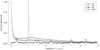 |
Fig. 4 Fourier spectra of electric field components in the plasma frequency experiment, showing clear peaks at 1ωe, indicating accurate capture of the plasma frequency. |
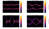 |
Fig. 5 Evolution of the two-stream instability, showing macro particle density in phase space at four distinct times, smoothed with a Gaussian filter. The transition from the linear phase to the non-linear phase is visible around t = 20ωe. |
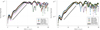 |
Fig. 6 Growth rate of the spectral component kmax of the electric field across simulations, organized by cell count (left) and particles per cell (right). |
4.3 Current sheet
To validate the robustness of our implementation under different PAC scenarios, we conducted a test focusing on a well-known plasma configuration: the current sheet. Current sheets naturally form in magnetized plasmas and are prone to instabilities that drive magnetic reconnection. This makes them an ideal test case, as even small variations in physical parameters can lead to noticeable differences in system evolution. Additionally, current sheets are widely studied in both space and solar physics under various levels of realism (Popescu Braileanu & Keppens 2023; Liu et al. 2022; Ji et al. 2022; Daldorff et al. 2022).
For this validation, we used a simplified setup inspired by Hawley & Stone (1995). The magnetic field profile is initialized using two hyperbolic tangent functions:
![Mathematical equation: $B_(x)(y)={[-B_(0)tanh((y+3.6)/(0.5.L))," if "y < 0","],[B_(0)tanh((y-3.6)/(0.5*L))," if "y >= 0","]:}$](/articles/aa/full_html/2025/04/aa52117-24/aa52117-24-eq39.png) (24)
(24)
where B0 = 25 G is the background magnetic field strength, and L is the initial width of the current sheets. Electrons and protons are initialized with Maxwellian velocity distributions at T = 1 MK and a uniform density of n = 109 cm−3 in a domain spanning [25.6, 12.8]rp. Periodic boundary conditions are applied along both the x and y axes. An initial velocity perturbation:
 (25)
(25)
with V0 = 0.001 in code units, is introduced to initiate reconnection. The resulting pressure imbalance leads to the collapse of the current sheet and the onset of reconnection.
The simulation was run to a code time of t = 200, corresponding to approximately 2.5 μs in real-time.
We performed experiments with varying grid resolutions ([128 × 64, 256 × 128, 512 × 256, 1024 × 512, 2048 × 1024]) and different numbers of particles per cell (ppc = [32, 64, 128, 256, 512]). In all cases, we used patches with 16 × 16 cells.
To ensure that the system behaves consistently across different PAC choices, six distinct scaling scenarios were tested. The PAC factors applied in each run are summarized in Table 2. Reducing the speed of light by a factor of 10 effectively reduces key dynamical scales, such as the proton gyro-radius, by the same factor. To maintain consistency in the physical size of the plasma structures, the elementary charge was also scaled accordingly in setups with a reduced speed of light. This ensures that fundamental spatial plasma scales remain identical across all experiments. However, due to this change, the Debye length increases by a factor of 10, while the plasma frequency decreases by the same factor.
The simulations were designed such that rp = 1 in all cases, with mass density normalized to ρ = 1 and time has been scaled so that c = 1 in experiments using [c10, c10m400, c10m100], and c = 10 in experiments using [pure, m400, m100]. This approach ensures that real-to-code unit conversions remain consistent across different runs, making comparisons straightforward.
Figure 7 shows the total current density at t = 150 for the six different PAC scenarios, while Figure 8 presents the temporal evolution for four selected PAC cases. In all runs, the current sheets become unstable and form plasmoids, but the rate of formation and the final plasmoid size vary depending on the PAC parameters.
Reducing the electron-to-proton mass ratio generally results in more diffused plasmoids. Since higher-mass electrons experience weaker interactions with the magnetic field, they contribute to increased diffusion. Adjusting the speed of light and elementary charge has a similar effect.
To further investigate PAC effects, we examined the reconnection rate, shown in Figure 9. For comparison, we also included a run where resampling was applied every 100 updates. The dimensionless reconnection rate was measured by averaging the vertical velocity at y = 3.6 ± 2 and y = –3.6 ± 2 and normalizing it to the background Alfvén velocity.
In all cases, the reconnection rate decreases when the electron-to-proton mass ratio is reduced. However, altering the speed of light produces a different effect. In the pure and m400 runs, the reconnection rate starts low, then rises sharply, peaking around 0.3 in the pure case before stabilizing around 0.2. In contrast, the c10 run shows a higher initial reconnection rate that later flattens out around 0.2.
Overall, these tests confirm that the implementation remains physically reasonable under various PAC choices. While PAC inevitably influences small-scale dynamics, the results remain qualitatively consistent, validating that the solver correctly accounts for kinetic and large-scale processes across different scaling regimes.
Physical adjustment of constants (PAC) factors for different simulation runs.
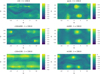 |
Fig. 7 Total current density for the six PAC scenarios at t = 150, with a resolution of 512 × 256 cells and 32 particles per cell. Differences in plasmoid formation highlight PAC effects. |
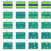 |
Fig. 8 Total current density evolution for four PAC scenarios at selected times, with 512 × 256 cells and 32 particles per cell. Axes and colour bar are identical to Figure 7. |
 |
Fig. 9 Reconnection rate using 512 × 256 cells and 32 particles per cell for the six PAC factors, and for the c10 run with resampling enabled (c10_re). |
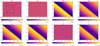 |
Fig. 10 Fast magnetosonic wave test at |

5 Coupling validation
In our coupling tests, we use the Bifrost MHD solver. The Bifrost solver is run using 4th-order stagger operations. The PIC solver similarly uses the 4th-order field solver. For mesh deposition and interpolation, we use Piecewise-Cubic-Spline. The higher- order scheme helps dampen waves and smooth out particle noise, which helps make the coupling smoother. We use the HL unit system in the coupling tests presented.
5.1 Fast magnetosonic wave
We use a setup similar to Makwana et al. (2017):
 (26)
(26)
 (27)
(27)
 (28)
(28)
 (29)
(29)
 (30)
(30)
 (31)
(31)
 (32)
(32)
 (33)
(33)
Here  is the wave speed, with va and cs being the Alfvén and sound speed respectively. We use γ = 5/3 and δ = 0.05. The wave numbers are kx = 2π/Lx and ky = 2π/Ly with
  is the frequency of the wave. Unlike in Makwana et al. (2017), the time-dependent oscillations must be added in our initial conditions as the PIC values are staggered in time. We use the same box size of Lx = 50di and Ly = 40di in the ranges –10 ≤ x ≤ 40 and –10 ≤ y ≤ 30 and a resolution of 500 × 400cells with size 0.1Δdi.
We use a number density of n0 = 109cm–3, a magnetic fields strength of B0 ≈ 6.28G, and a temperature of Ti = Te = 1.14 * 107K. We scale ϵ0 with a factor of 100, reducing the speed of light by a factor of 10. We use an electron-to-proton mass ratio of 20, meaning we increase the mass of the electrons with a factor of 91.8. We normalize mass density such that ρ0 = 1 in code units. We normalize length scales so di = 1 in code units, and finally, we normalize time such that C = 1, which in this case also gives us ωi = 1. These choices of PAC, and normalization give us the same code units for the magnetic field, pressure, and mass density as in Makwana et al. (2017): ρ0 = 1.0, p = 0.0002 and B0 = 0.05.
The MHD patches in the region 0 ≤ x ≤ 20 and 0 ≤ y ≤ 20 create PIC patches during initialization. We use 1024 particles per cell per species. The PIC region is indicated by the black square in Figure 10. We show the evolution of the wave at time t = 600ωi (1.02 wave periods) in Figure 10. To further investigate we show a 1D trace line in the wave direction in Figure 11. The trace line is indicated by the red line in Figure 10.
The results show excellent agreement between the coupled run and the pure MHD run. The noise in the constant components (bx,by,vz) remains within the PIC region and does not cause perturbations outside it. At the snapshot time, the wavefront is within the PIC region. The sharp gradient is well captured in PIC, although it is slightly more diffusive than in the pure MHD run. The wavefront (now a shock), causes some spurious oscillation in the pic region, most clear in the bz and vy component at the ‘top’ of the wavefront, but the perturbation is not much larger than general PIC noise.

5.2 Circular polarized Alfvén wave
Our second coupling test is a circularly polarized Alfvén wave, using a setup similar to Makwana et al. (2017):
 (34)
(34)
 (35)
(35)
 (36)
(36)
 (37)
(37)
 (38)
(38)
 (39)
(39)
 (40)
(40)
 (41)
(41)
We use the same PAC and normalization as in the fast wave test. But, we double the strength of the magnetic field to B0 = 12.56G. This results in the code units: ρ0 = 1.0, p = 0.0002 and B0 = 0.1. The simulation domain is also identical to our fast wave test - meaning our simulation size is half that of Makwana et al. (2017), but with the same number of grid points. We again, use 1024 particles per cell.
The initial conditions are rotated by an angle θ = tan–1(Lx/Ly). We show the evolution of the wave at time t = 800ωi (1.12 wave periods) in Figure 12 and we trace a 1D line along the wave direction in Figure 13. The trace line is indicated by the red line in Figure 12.
There is very little distortion at the PIC-MHD interface in the magnetic field and velocity components. The PIC region tends to be more diffusive, and the wave travels slightly slower than in the pure MHD, which can be seen in Figure 13. The noise in pressure and density generates waves at the interface, which travels in the MHD domain. The amplitude of the waves remains at the same level as the PIC noise and does not affect the evolution of the wave much. Otherwise, there is excellent agreement between pure MHD and the coupled setup.
6 Discussions
6.1 Speed of light and related issues
The integration of the PIC solver within the DISPATCH framework marks our first step towards simulating the complex plasma dynamics of solar flares. This integration also highlights certain limitations inherent to the nature of explicit solvers, particularly as they relate to the DISPATCH code framework.
A primary challenge is the constraint on time step size due to the speed of light, which is necessary for accurately simulating electromagnetic field propagation. This constraint, while potentially limiting in other, less extreme contexts, aligns well with the solver’s intended application to scenarios involving relativistic particle acceleration, as observed in solar flares. Realistically modelling such scenarios requires embracing the full range of velocities involved.
Moreover, relativistic conditions present certain advantages, such as reducing the impact of the mass difference between electrons and ions, as the two species move at nearly the same velocities, despite their large mass disparity.
The solver’s reliance on uniform time steps diverges somewhat from DISPATCH’s otherwise innovative approach with local time stepping. To some extent, this is an unavoidable consequence of the fundamental impact of the speed of light in relativistic dynamics - when information speed is essentially constant, there is less to gain from variations in speed. However, the framework still allows for large differences in time steps due to spatial resolution or different requirements from the physics modelled in each patch.
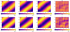 |
Fig. 12 Alfven wave at |


6.2 Exposing the consequences of PAC
The adjustment of physical constants (PAC) is commonly used in PIC simulations but often lacks transparency, making it difficult to assess its impact on physical accuracy. Our approach ensures explicit documentation of scaling choices, enabling a systematic evaluation of PAC’s effects.
We examined how modifying the speed of light and the electron mass influences plasma dynamics. Our results show that applying PAC to reduce scale differences systematically reduces the peak reconnection rate, with more pronounced effects at lower electron-to-proton mass ratios. Previous studies (Hesse et al. 2018) found that reconnection rates are primarily determined by large-scale ion flows and thus do not depend on the electron mass. While our results confirm that the long-term reconnection rate is only mildly affected, we find that the peak rate can be significantly altered, particularly when multiple PAC modifications are combined.
The impact of PAC may be even more pronounced in PIC- MHD coupling, as realistic setups will require significant PAC adjustments. This underscores the need for careful selection of scaling parameters and transparency in hybrid modelling to ensure consistency across kinetic and macroscopic scales. Future work will further explore these effects in embedded PIC- MHD simulations, assessing PAC’s role in realistic reconnection scenarios.
6.3 Coupling
The results presented here constitute a successful demonstration of our coupling scheme between the PIC solver and MHD within DISPATCH. Our approach employs weighted field averaging at the PIC-MHD interfaces, ensuring a smooth transition between the kinetic and fluid regions. The test cases confirm that propagating waves are accurately captured across the interface with minimal boundary artefacts, highlighting the robustness of our coupling strategy in controlled setups.
In the current implementation, PIC patches are statically embedded within a uniform mesh and remain active throughout the simulation. This static configuration provides a stable environment for validating the coupling mechanism; however, it does not yet leverage the full flexibility of DISPATCH. The framework allows for dynamic activation and deactivation of solvers. Once implemented, this will enable PIC patches to be placed adaptively in regions where kinetic effects are critical. This will further optimize computational efficiency while preserving fine-scale physics where needed.
A key motivation for this coupling approach is to bridge the gap between large-scale MHD dynamics and small-scale kinetic processes in solar flare simulations. With the immense disparity between global and kinetic scales, embedding PIC within an adaptive MHD framework offers a computationally viable way to capture reconnection physics without requiring fully kinetic simulations. The results in our test cases indicate that this strategy is effective, while further work is needed to refine the dynamic criteria for activating PIC patches.
Future work will focus on developing a truly adaptive coupling strategy that dynamically refines regions requiring kinetic treatment. This will allow the simulation to transition seamlessly between MHD and PIC descriptions based on evolving plasma conditions, rather than relying on predefined regions. Additionally, testing in more complex, realistic solar flare configurations will be necessary to ensure the robustness of the method in astrophysical contexts.
7 Conclusions
We have successfully implemented a hybrid PIC/MHD solver setup in the DISPATCH code framework and subjected it to a comprehensive set of tests and validations, including tests that
validate specific field and particle mechanism separately;
validate the variation of characteristic problem scales when varying fundamental physical constants (PAC scalings; cf. Table 2);
uses fundamental plasma oscillations to validate electric field forces and charged particle dynamics;
reveals the influence of particle resampling;
reveals the influence of cell per wavelength and particles per cell on wave propagation and damping;
uses the current sheet and two-stream instabilities to validate the full PIC solver;
validate the coupling between the PIC and MHD solvers, using fast magnetosonic waves and circularly polarized Alfvén waves.
These results confirm the solver’s robustness and accuracy and establish the ability of the hybrid PIC/MHD setup to capture key particle-field interactions and electromagnetic dynamics, providing a strong foundation for affordable, yet realistic hybrid plasma simulations.
A critical aspect of our study is the examination of the effects of scale ratio modifications (PAC effects) on plasma behaviour, particularly on reconnection rates. While PAC offers a practical means to make kinetic simulations computationally more feasible, our results highlight that it also potentially alters key plasma properties, which must be carefully accounted for. By explicitly documenting our scaling choices, we provide a transparent framework for future studies to evaluate and mitigate potential biases introduced by PAC.
Beyond validating the PIC solver itself, this work also demonstrates a successful coupling strategy between PIC and MHD solvers within the DISPATCH code framework. Our interface treatment ensures smooth transitions between kinetic and fluid regions, laying the groundwork for large-scale solar flare simulations that integrate kinetic reconnection physics within a global MHD framework. The ability to selectively resolve kinetic effects where needed represents a significant step towards a more comprehensive and computationally efficient approach to solar flare modelling.
Moving forward, our focus will be on refining the dynamic activation of PIC patches, improving adaptive refinement strategies, and applying the hybrid PIC-MHD approach to realistic solar flare environments. By bridging the gap between large- scale flare evolution and the microphysics of reconnection, this work paves the way for a more complete understanding of solar flare dynamics.
Acknowledgements
We would like to thank Troels Haugblle for his invaluable discussions and insights regarding the PhotonPlasma code and plasma physics. We also wish to acknowledge Jan Truelsen for his assistance and contributions to the theoretical foundations of this work, particularly insight into the warm case analysis of the two-stream instability test. Additionally, we thank Andrius Popovas and Mikolaj Szydlarski for their guidance and support throughout the code development process. During the preparation of this work we used ChatGPT in order to enhance the clarity of writing. After using this tool, we reviewed and edited the content as needed and take full responsibility for the content of the published article. This research was supported by the Research Council of Norway through its Centres of Excellence scheme, project number 262622.
References
- Baumann, G., Haugbølle, T., & Nordlund, A. 2013, ApJ, 771, 93 [Google Scholar]
- Birdsall, C. K., & Langdon, A. B. 1991, Plasma Physics via Computer Simulation, The Adam Hilger Series on Plasma Physics (Bristol: Adam Hilger) [Google Scholar]
- Carron, N. 2015, arXiv e-prints [arXiv:1506.01951] [Google Scholar]
- Chen, Y., Tóth, G., Zhou, H., & Wang, X. 2023, Comput. Phys. Commun., 287, 108714 [Google Scholar]
- Courant, R., Friedrichs, K., & Lewy, H. 1928, Math. Ann., 100, 32 [Google Scholar]
- Cui, C., Huang, Z., Hu, Y., & Wang, J. 2019, in The 36th International Electric Propulsion Conference [Google Scholar]
- Daldorff, L. K., Tóth, G., Gombosi, T. I., et al. 2014, J. Computat. Phys., 268, 236 [Google Scholar]
- Daldorff, L. K. S., Leake, J. E., & Klimchuk, J. A. 2022, ApJ, 927, 196 [Google Scholar]
- Esirkepov, T.Zh. 2001, Comput. Phys. Commun., 135, 144 [Google Scholar]
- Feynman, R. P., Leighton, R. B., & Sands, M. 1965, Am. J. Phys., 33, 750 [Google Scholar]
- Fromang, S., Hennebelle, P., & Teyssier, R. 2006, A&A, 457, 371 [Google Scholar]
- Gudiksen, B. V., Carlsson, M., Hansteen, V. H., et al. 2011, A&A, 531, A154 [Google Scholar]
- Guo, F., Liu, Y.-H., Zenitani, S., & Hoshino, M. 2024, Space Sci. Rev., 220, 43 [Google Scholar]
- Harris, E. G. 1962, Il Nuovo Cimento, 23, 115 [Google Scholar]
- Haugbølle, T., Frederiksen, J. T., & Nordlund, Å. 2013, Phys. Plasmas, 20, 062904 [Google Scholar]
- Hawley, J. F., & Stone, J. M. 1995, Numer. Methods Astrophys. Hydrodyn., 89, 127 [Google Scholar]
- Hazeltine, R. D., & Waelbroeck, F. L. 1998, Frontiers in Physics, 100, The Framework of Plasma Physics (Reading, MA: Perseus Books) [Google Scholar]
- Hesse, M., Schindler, K., Birn, J., & Kuznetsova, M. 1999, Phys. Plasmas, 6, 1781 [Google Scholar]
- Hesse, M., Liu, Y.-H., Chen, L.-J., et al. 2018, Phys. Plasmas, 25, 032901 [Google Scholar]
- Ji, H., Daughton, W., Jara-Almonte, J., et al. 2022, Nat. Rev. Phys., 4, 263 [Google Scholar]
- Ji, L., Yang, Z., Li, Z., et al. 2023, J. Math. Phys., 64, 063503 [Google Scholar]
- Kane Yee. 1966, IEEE Trans. Antennas Propag., 14, 302 [Google Scholar]
- Klion, H., Jambunathan, R., Rowan, M. E., et al. 2023, ApJ, 952, 8 [Google Scholar]
- Lapenta, G., Brackbill, J. U., & Ricci, P. 2006, Phys. Plasmas, 13, 055904 [Google Scholar]
- Liu, Y.-H., Cassak, P., Li, X., et al. 2022, Commun. Phys., 5, 97 [Google Scholar]
- Makwana, K., Keppens, R., & Lapenta, G. 2017, Comput. Phys. Commun., 221, 81 [Google Scholar]
- Malakit, K., Shay, M. A., Cassak, P. A., & Bard, C. 2010, J. Geophys. Res.: Space Phys., 115 [Google Scholar]
- Markidis, S., Henri, P., Lapenta, G., et al. 2014, J. Computat. Phys., 271, 415 [Google Scholar]
- Miyoshi, T., & Kusano, K. 2005, J. Computat. Phys., 208, 315 [Google Scholar]
- Muraviev, A., Bashinov, A., Efimenko, E., et al. 2021, Comput. Phys. Commun., 262, 107826 [Google Scholar]
- Nordlund, A., Ramsey, J. P., Popovas, A., & Küffmeier, M. 2018, MNRAS, 477, 624 [Google Scholar]
- Popescu Braileanu, B., & Keppens, R. 2023, A&A, 678, A66 [Google Scholar]
- Popovas, A., Nordlund, Å., & Szydlarski, M. 2022, A&A, submitted [arXiv:2211.09564] [Google Scholar]
- Ripperda, B., Bacchini, F., Teunissen, J., et al. 2018, Astrophys. J. Suppl., 235, 21 [Google Scholar]
- Selvi, S., Porth, O., Ripperda, B., et al. 2023, ApJ, 950, 169 [Google Scholar]
- Smets, R., Aunai, N., Ciardi, A., et al. 2021, Comput. Phys. Commun., 261, 107666 [Google Scholar]
- Teyssier, R. 2002, A&A, 385, 337 [NASA ADS] [CrossRef] [EDP Sciences] [Google Scholar]
- Vay, J.-L. 2008, Phys. Plasmas, 15, 056701 [Google Scholar]
- Zharkova, V. V., Arzner, K., Benz, A. O., et al. 2011, Space Sci. Rev., 159, 357 [Google Scholar]
All Tables
All Figures
|
Fig. 1 Time staggering of the explicit PIC solver in DISPATCH, illustrating the integration order. The electric field is staggered by a full time step, Δt in the past. Magnetic field, particle velocities, and current density are staggered backwards by 0.5Δt. Particle position is centred in time. |
| In the text | |
|
Fig. 2 Spatial staggering of mesh variables on a Yee lattice. Magnetic fields are located on the cell faces, electric fields, and current densities on the edges, with mass density, momentum, and energy centred within each cell. Charge density is uniquely staggered to the lower corner of each cell. |
| In the text | |
|
Fig. 3 Illustration of particle sampling in a 2D setup with 10 particles per cell. Each cell is divided into |
| In the text | |
|
Fig. 4 Fourier spectra of electric field components in the plasma frequency experiment, showing clear peaks at 1ωe, indicating accurate capture of the plasma frequency. |
| In the text | |
|
Fig. 5 Evolution of the two-stream instability, showing macro particle density in phase space at four distinct times, smoothed with a Gaussian filter. The transition from the linear phase to the non-linear phase is visible around t = 20ωe. |
| In the text | |
|
Fig. 6 Growth rate of the spectral component kmax of the electric field across simulations, organized by cell count (left) and particles per cell (right). |
| In the text | |
|
Fig. 7 Total current density for the six PAC scenarios at t = 150, with a resolution of 512 × 256 cells and 32 particles per cell. Differences in plasmoid formation highlight PAC effects. |
| In the text | |
|
Fig. 8 Total current density evolution for four PAC scenarios at selected times, with 512 × 256 cells and 32 particles per cell. Axes and colour bar are identical to Figure 7. |
| In the text | |
|
Fig. 9 Reconnection rate using 512 × 256 cells and 32 particles per cell for the six PAC factors, and for the c10 run with resampling enabled (c10_re). |
| In the text | |
|
Fig. 10 Fast magnetosonic wave test at |
| In the text | |
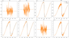 |
Fig. 11 Trace line for the fast magnetosonic wave test at |
| In the text | |
|
Fig. 12 Alfven wave at |
| In the text | |
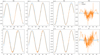 |
Fig. 13 Trace line for the fast alfven wave test at |
| In the text | |
Current usage metrics show cumulative count of Article Views (full-text article views including HTML views, PDF and ePub downloads, according to the available data) and Abstracts Views on Vision4Press platform.
Data correspond to usage on the plateform after 2015. The current usage metrics is available 48-96 hours after online publication and is updated daily on week days.
Initial download of the metrics may take a while.