| Issue |
A&A
Volume 695, March 2025
|
|
|---|---|---|
| Article Number | L24 | |
| Number of page(s) | 5 | |
| Section | Letters to the Editor | |
| DOI | https://doi.org/10.1051/0004-6361/202453530 | |
| Published online | 25 March 2025 | |
Letter to the Editor
Helical flows along coronal loops following the launch of a coronal mass ejection
1
Astronomy & Astrophysics Section, School of Cosmic Physics, Dublin Institute for Advanced Studies, DIAS Dunsink Observatory, Dublin D15 XR2R, Ireland
2
Centre for Astrophysics and Relativity, School of Physical Sciences, Dublin City University, Glasnevin Campus, Dublin D09 V209, Ireland
3
Mullard Space Science Laboratory, University College London, Holmbury St Mary, Dorking, Surrey RH5 6NT, UK
4
Konkoly Observatory, Research Centre for Astronomy and Earth Sciences, Hungarian Academy of Sciences, Konkoly Thege út 15-17, H-1121 Budapest, Hungary
⋆ Corresponding author; mohamed.nedal@dias.ie
Received:
19
December
2024
Accepted:
22
February
2025
Context. Solar flares and coronal mass ejections (CMEs) are manifestations of energy release in the solar atmosphere. They can be accompanied by dynamic mass motions and waves in the surrounding atmosphere.
Aims. We present observations of plasma moving in a helical trajectory along a set of coronal loops formed following the eruption of a CME on 2024 May 14. This helical motion was observed in extreme ultraviolet images from the Solar Dynamics Observatory (SDO) and provides new insights into plasma properties in a set of post-eruption coronal loops.
Methods. We utilized images from the SDO Atmospheric Imaging Assembly (AIA) instrument to track the helical motion of plasma and to characterize its speed, acceleration, and physical properties. Additionally, we explored the evolution of the plasma density and temperature along the helical structure using the differential emission measure technique.
Results. The helical structure was visible to AIA for approximately 22 minutes; it had a diameter of ∼22 Mm and a total trajectory of nearly 184 Mm. According to our analysis of the AIA observations, the speed of the plasma flow along this helical coronal loop ranged from 77 to 384 km s−1, temperatures from 3.46 to 10.2 MK, densities from 4.3 × 10⁶ to 1.55 × 107 cm−3, and the magnetic field strength from 0.05 to 0.3 G.
Conclusions. Following the launch of the CME, we find clear evidence for impulsive heating and expansion of the plasma, which travelled along a helical trajectory along a set of post-eruption loops. These observations provide an insight into impulsive plasma flows along coronal loops and the topology of coronal loops.
Key words: Sun: activity / Sun: corona / Sun: coronal mass ejections (CMEs) / Sun: filaments / prominences / Sun: flares / Sun: EUV radiation
© The Authors 2025
 Open Access article, published by EDP Sciences, under the terms of the Creative Commons Attribution License (https://creativecommons.org/licenses/by/4.0), which permits unrestricted use, distribution, and reproduction in any medium, provided the original work is properly cited.
This article is published in open access under the Subscribe to Open model. Subscribe to A&A to support open access publication.
1. Introduction
Coronal mass ejections (CMEs) are massive eruptions of plasma and magnetic fields from the Sun’s corona that disturb the heliosphere and drive space weather phenomena at the Earth. Complex structures, such as loops and helical flux ropes, as well as phenomena resembling massive vortices or tornado-like formations, often accompany CME evolution, specifically in the solar corona (Su et al. 2013; Vourlidas 2014; Chen 2017; Devi et al. 2021). These whirling plasma formations, linked to twisted magnetic fields and magnetic reconnection, offer valuable insights into solar eruption mechanisms (Chen et al. 2017; Cheng et al. 2017).
Solar tornadoes arise from swirling magnetic fields in the Sun’s atmosphere and are often linked to the barbs of solar prominences (Wedemeyer et al. 2013; Engvold 2015). Up to 30 tornadoes can be active at any given time, particularly during solar maximum, serving as plasma sources or sinks for prominences (Su et al. 2012; Wedemeyer et al. 2013). Their predominantly vertical, helical magnetic fields indicate a dynamic relationship with prominences, as intermittent rotation may contribute to instability and eruptions (González et al. 2016; Levens et al. 2016).
Solar tornadoes are pivotal in supplying mass and twist to filaments, influencing their formation and eruptions (Su et al. 2012; Gunár et al. 2023). Magnetic twist, rotation, plasma-β, and viscosity significantly impact their dynamics, with magnetic twist dominant in coronal conditions and rotation more relevant in the photosphere (Mozafari Ghoraba et al. 2018). Despite the growing understanding of solar tornadoes, questions remain about their role in coronal heating and the detailed processes of magnetic reconnection (Pontin 2012; Panesar et al. 2013; Kuniyoshi et al. 2024). Comprehensive studies on solar tornado-like structures must consider their three-dimensional, non-uniform, and asymmetric evolution (Su et al. 2013; Schmieder et al. 2017).
We present a high-resolution observation of a helical mass motion formation in the solar corona that occurred following a solar flare and CME eruption. To the best of our knowledge, this is the first time a helical flow has been clearly identifiable during the eruption of a CME event. This may offer new insights into and constraints on CME models and mass-energy transport during eruptions. In Sect. 2 we describe the observations and data analysis techniques employed in this study. In Sect. 3 we present and interpret the results. Finally, in Sect. 4 we summarize our findings.
2. Observations and data analysis
The Solar Dynamics Observatory (SDO)’s Atmospheric Imaging Assembly (AIA) provides continuous high-resolution imaging of the Sun’s atmosphere using multi-wavelength channels (Pesnell et al. 2012; Lemen et al. 2012). The extreme ultraviolet (EUV) channels in various ionized iron states allow the construction of temperature maps of the solar corona, ranging from below 1 MK to above 20 MK. The 304 Å channel, which captures emissions from ionized helium (He II), is particularly important for studying prominences, filaments, and chromospheric dynamics. AIA captures images up to 0.5 R⊙ above the solar limb with a spatial resolution of about 1.5 arcseconds and a 12-second cadence, enabling precise tracking of dynamic phenomena such as plasma flows and tornadoes. Its multi-wavelength imaging enables multi-thermal diagnostics across various heights in the solar atmosphere.
The plasma flow began forming on 2024 May 14 at ∼17:10 UT during a CME event from active region 13682 (E65N17). The active region had an area of 100 Mm2, according to NOAA1. The associated halo CME was detected by the Solar and Heliospheric Observatory (SOHO) Large Angle and Spectrometric Coronagraph (LASCO) C2 at 17:48:05 UT, with a linear speed of 1407 km s−1 and an acceleration of −40.3 m s−2 as per the CDAW CME catalogue2. The CME was also associated with an M4.4-class flare (start: 17:25 UT, peak: 17:38 UT, end: 18:18 UT). Figure 1 illustrates the helical evolution over four timesteps in three EUV channels, showing a twisted structure spanning ∼184 Mm.
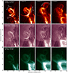 |
Fig. 1. AIA images of the helical plasma in three channels that represent low (top row), medium (middle row), and high (bottom row) coronal temperatures. The white arrows in the top row show the direction of the plasma motion. Movies of the event are available online. |
First, we obtained level-1 AIA data. We then used the aiapy Python package to upgrade the AIA data to level 1.5 and apply point spread function convolution. We tracked the evolution of the plasma flow along the structure in the 304 Å passband using Bézier curves (Mortenson 1999), stacking the intensities with time to produce J plots, as shown in Fig. 2. By using a quadratic model to fit the bright structure in the J plots, we estimated the projected speeds of the plasma motion in the four segments, from F1 to F4, assuming constant acceleration. We calculated the initial position (s0), initial velocity (v0), acceleration (a), and instantaneous velocity (v(t)) from the curve fitting. We then computed the propagated uncertainties for minimum velocity (vmin), maximum velocity (vmax), and mean velocity (vmean). The flow exhibited anti-clockwise rotation at a projected velocity of ∼155 ± 26 km s−1. These are projected speeds due to the flow’s position near the solar limb, which limits line-of-sight accuracy.
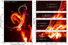 |
Fig. 2. Time-dependent height analysis of four segments along the plasma helical structure. Left: Snapshot image of the helical motion in four segments. Right: J plots of the initial velocities (in km s−1) and acceleration (in m s−2) of the plasma in the four segments. |
Differential emission measure (DEM) analysis is a robust technique for studying coronal plasma temperature distributions. Various methods address its ill-posed inverse problem, including fast regularized inversion (Plowman et al. 2013), enhanced algorithms with error estimates (Hannah & Kontar 2013), and linear programming approaches (Cheung et al. 2015). Recent advancements, such as a regularized maximum likelihood method (Massa et al. 2023), improve computational speed, noise robustness, and error estimation, enabling routine DEM map production for detailed studies of coronal thermal structures. Compared to earlier techniques (Withbroe 1975; Sylwester et al. 1980; Siarkowski 1983), these methods provide more reliable insights into multi-thermal plasma environments.
Despite its strengths, DEM analysis has limitations, including errors from noise and multi-thermality ambiguities that affect temperature resolution (Guennou et al. 2012). By combining DEM analysis with solar rotational tomography (Frazin et al. 2005), 3D coronal temperature maps can be produced. For instance, Sun et al. (2014) studied an M7.7 flare, finding peak emission near the loop top at ∼16 MK. Levens et al. (2015) applied DEM analysis to a solar tornado, revealing temperature-dependent velocity patterns and electron density distributions.
We used the regularized inversion of Hannah & Kontar (2013) to investigate the temporal and spatial evolution of the plasma flow’s thermal structure. From the DEM results, we computed the average temperature (Tavg) and electron density (ne) for each pixel using DEM-weighted averages. The line-of-sight depth, estimated from the observed plasma structure and based on the first plasma loop’s apparent diameter, was 2.24 × 109 cm.
Using Tavg and ne, we calculated the thermal pressure (Pth, in dyne cm−2) and sound speed (Cs, in km s−1). Assuming the plasma speed approximates the Alfvén speed (vA ≈ v), we inferred the magnetic field strength (in gauss) in the flow’s four segments and estimated the magnetic pressure (Pm, in dyne cm−2). The plasma-β parameter, representing the ratio of thermal to magnetic pressure, was calculated for the four segments of the helical flow. The minimum plasma-β ranged from 0.89 to 18.19, and the maximum ranged from 1.87 to 119.13. The mean values for the segments were as follows: F1 (55.37), F2 (2.79), F3 (13.89), and F4 (1.33). The plasma flow’s four segments exhibited mean temperatures ranging from 2.46 × 10⁶ K to 4.74 × 10⁶ K and mean electron densities from 2.91 × 106 cm−3 to 7.93 × 106 cm−3.
3. Results and discussion
The helical flow observed during the early stages of the CME eruption exhibited notable stability in size while undergoing significant rotational motion. Multi-wavelength observations revealed that the flow was closely tied to the underlying magnetic field structure, likely a segment of a flux rope. The rotational motion, evident in the AIA 304 Å observations, spanned from 17:17–17:41 UT, progressing through four distinct segments of the helical flow structure. J maps constructed for these segments reveal spiralling plasma motions, with speeds varying significantly across the structure. The loops corresponding to segments F2 and F4 exhibited the highest speeds, ranging from 297 to 384 km s−1, while segments F1 and F3 displayed steadier, lower velocities, averaging 50–88 km s−1, indicative of more stable magnetic configurations. These variations likely reflect differences in local magnetic field configurations and reconnection dynamics.
The plasma dynamics and velocity distribution of the helical flow suggest a complex interaction between the local magnetic topology and energy release processes. DEM analysis shows that the helical plasma flow had a stratified thermal structure across temperature bins (Fig. 3). At lower temperatures (log(T) = 5.6 − 6.2), the flow exhibited intricate structures with moderate DEM values, indicating a condensed, cooler plasma. The DEM was higher in areas of intermediate temperatures (log(T) = 6.2 − 6.8), particularly in the core of the helical flow, suggesting significant plasma heating. At higher temperatures (log(T) = 6.8 − 7.4), the DEM became highest in the lower helical flow region, where flare ribbons and loops appeared, with values typical of flare-related heating above 10 MK. These trends align with scenarios of magnetic reconnection or shock heating during the event (Longcope 2005; Aschwanden & Boerner 2011; Schmelz et al. 2013).
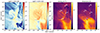 |
Fig. 3. DEM analysis of the helical flow at a single time frame at 17:36 UT. Left panels: DEM output in two temperature ranges. Right panels: density and mean temperature deduced from the DEM analysis. Associated movies are available online. |
The plasma density distribution further highlights the helical plasma’s stratified nature. Densities reached 107 cm−3 in the flow’s core, with steep gradients towards the periphery. The highest densities corresponded to localized areas of strong plasma emission, implying magnetic confinement or accumulation due to reconnection processes. The mean temperature map corroborated this, with the hottest regions overlapping the densest areas, consistent with localized energy deposition. These findings align with previous studies of solar eruptive structures, where plasma heating and energy release are concentrated in confined magnetic regions before dissipating (Galeev et al. 1981; Susino et al. 2010; Reale 2014).
The temporal evolution of thermal and magnetic pressures reveals distinct responses across the flow segments (Fig. 4). The thermal pressure dominated in F1 during impulsive heating, peaking at around 17:34 UT, while the magnetic pressure played a stabilizing role in F2 and F4. Plasma-β values further confirm that thermal pressure dominated in F1 and F3 (β ≫ 1), whereas F2 and F4 exhibited a balanced interplay between thermal and magnetic forces (β ∼ 1).
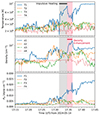 |
Fig. 4. Temporal evolution of key plasma parameters along the four segments of the helical structure. From top to bottom, we have the mean temperature, density, and thermal pressure at the four points (n1–n4 and T1–T4) along the plasma flow path shown in Fig. 3. |
Our results suggest that impulsive heating, triggered by the accompanying M-class flare, played a pivotal role in driving plasma evaporation and motion along pre-existing magnetic field structures, which is consistent with the findings of Long et al. (2023). The rapid heating from ∼2 MK to ∼9 MK, followed by a density rise from ∼106 cm−3 to ∼4 × 106 cm−3, highlights the role of flare energy release in plasma dynamics. This behaviour parallels findings of explosive heating and chromospheric evaporation in low-density coronal plasma (Bradshaw & Cargill 2006).
The observations suggest that the plasma predominantly filled pre-existing magnetic structures without significant evolution of the magnetic field itself. The flow’s behaviour differed from that of the rapidly reforming flux ropes described by Janvier et al. (2014). Instead, the observed plasma motion appears to result primarily from heating and overpressure effects induced by the eruption.
4. Conclusions
The helical mass motions observed following the CME eruption are an excellent demonstration of how complex formations interact with magnetic field structures and energy release processes. The flow’s thermal stratification, density gradients, and velocity changes indicate how magnetic reconnection and impulsive heating shape its dynamics.
Key findings suggest that rapid plasma heating and evaporation, driven by the accompanying M-class flare, were integral to the helical flow’s behaviour. While the observed motion and plasma flows align with solar tornado characteristics, the lack of significant magnetic evolution and the plasma’s confinement to pre-existing structures point to a response dominated by CME-induced compression and overpressure effects rather than a fully developed tornado-like dynamic.
The velocity of the plasma flow ranged from 50 to 384 km s−1, with stratified thermal structure and densities peaking at 107 cm−3. Thermal pressure dominated in some regions (β ≫ 1), while others displayed a balance between thermal and magnetic forces (β ∼ 1). The estimated magnetic field strength was significantly weaker than that of typical coronal loops, potentially due to projection effects, assumptions equating plasma velocity to the Alfvén speed, or DEM-based uncertainties in density estimation. It is clear to us that the impulsive heating followed by the density increase yielded a pressure impulse in the flow, which is consistent with the studies presented in the introduction.
These observations reinforce the idea that complex flows play a key role in mass and energy transport during eruptive events. However, further studies, particularly those incorporating direct magnetic field measurements, are needed to fully unravel the interplay between plasma dynamics, magnetic reconnection, and CME evolution.
Data availability
Movies associated to Figs. 1 and 3 are available at https://www.aanda.org
National Oceanic and Atmospheric Administration (NOAA) Space Weather Prediction Center (SWPC): https://www.swpc.noaa.gov/products/solar-and-geophysical-activity-summary
Coordinated data analysis workshops (CDAWs): https://cdaw.gsfc.nasa.gov/CME_list/
Acknowledgments
Many thanks to Pascal Demoulin for the insightful discussions. Thank you to Shane Maloney, Paul Wright, Alasdair Wilson, and Laura Hayes for their helpful suggestions. Thank you to the referee for the constructive feedback. We acknowledge using the Python-curated version (https://doi.org/10.5281/zenodo.13743565) of the regularized inversion of Hannah & Kontar (2013) to calculate DEM from AIA observations. We acknowledge the use of data from the SDO/AIA instrument. This research used version 6.0.2 (https://github.com/ianan/demreg) of the SunPy open source software package (The SunPy Community 2020). This research used version 0.8.0 (https://doi.org/10.5281/zenodo.5606094) of the aiapy open source software package (Barnes et al. 2020). This work also made use of Astropy: (http://www.astropy.org) a community-developed core Python package and an ecosystem of tools and resources for astronomy (Astropy Collaboration 2013, 2018, 2022). This work is supported by the project “The Origin and Evolution of Solar Energetic Particles”, funded by the European Office of Aerospace Research and Development under award No. FA8655-24-1-7392.
References
- Aschwanden, M. J., & Boerner, P. 2011, ApJ, 732, 81 [NASA ADS] [CrossRef] [Google Scholar]
- Astropy Collaboration (Robitaille, T. P., et al.) 2013, A&A, 558, A33 [NASA ADS] [CrossRef] [EDP Sciences] [Google Scholar]
- Astropy Collaboration (Price-Whelan, A. M., et al.) 2018, AJ, 156, 123 [Google Scholar]
- Astropy Collaboration (Price-Whelan, A. M., et al.) 2022, ApJ, 935, 167 [NASA ADS] [CrossRef] [Google Scholar]
- Barnes, W. T., Cheung, M. C. M., Bobra, M. G., et al. 2020, Journal of Open Source Software, 5, 2801 [Google Scholar]
- Bradshaw, S. J., & Cargill, P. J. 2006, A&A, 458, 987 [NASA ADS] [CrossRef] [EDP Sciences] [Google Scholar]
- Chen, H., Zhang, J., Ma, S., Yan, X., & Xue, J. 2017, ApJ, 841, L13 [NASA ADS] [CrossRef] [Google Scholar]
- Chen, J. 2017, Physics of Plasmas, 24, 090501 [NASA ADS] [Google Scholar]
- Cheng, X., Guo, Y., & Ding, M. 2017, Science China Earth Sciences, 60, 1383 [Google Scholar]
- Cheung, M. C. M., Boerner, P., Schrijver, C. J., et al. 2015, ApJ, 807, 143 [Google Scholar]
- Devi, P., Démoulin, P., Chandra, R., et al. 2021, A&A, 647, A85 [NASA ADS] [CrossRef] [EDP Sciences] [Google Scholar]
- Engvold, O. 2015, in Solar Prominences, eds. J. C. Vial, & O. Engvold, Astrophysics and Space Science Library, 415, 31 [NASA ADS] [Google Scholar]
- Frazin, R. A., Kamalabadi, F., & Weber, M. A. 2005, ApJ, 628, 1070 [Google Scholar]
- Galeev, A. A., Rosner, R., Serio, S., & Vaiana, G. S. 1981, ApJ, 243, 301 [Google Scholar]
- González, M. J. M., Ramos, A. A., Arregui, I., et al. 2016, ApJ, 825, 119 [CrossRef] [Google Scholar]
- Guennou, C., Auchère, F., Soubrié, E., et al. 2012, ApJS, 203, 26 [Google Scholar]
- Gunár, S., Labrosse, N., Luna, M., et al. 2023, Space Sci. Rev., 219, 33 [CrossRef] [Google Scholar]
- Hannah, I. G., & Kontar, E. P. 2013, A&A, 553, A10 [NASA ADS] [CrossRef] [EDP Sciences] [Google Scholar]
- Janvier, M., Aulanier, G., Bommier, V., et al. 2014, ApJ, 788, 60 [Google Scholar]
- Kuniyoshi, H., Bose, S., & Yokoyama, T. 2024, ApJ, 969, L34 [NASA ADS] [CrossRef] [Google Scholar]
- Lemen, J. R., Title, A. M., Akin, D. J., et al. 2012, Sol. Phys., 275, 17 [Google Scholar]
- Levens, P. J., Labrosse, N., Fletcher, L., & Schmieder, B. 2015, A&A, 582, A27 [NASA ADS] [CrossRef] [EDP Sciences] [Google Scholar]
- Levens, P. J., Schmieder, B., Labrosse, N., & López Ariste, A. 2016, ApJ, 818, 31 [NASA ADS] [CrossRef] [Google Scholar]
- Long, D. M., Green, L. M., Pecora, F., et al. 2023, ApJ, 955, 152 [CrossRef] [Google Scholar]
- Longcope, D. W. 2005, Living Reviews in Solar Physics, 2, 7 [Google Scholar]
- Massa, P., Emslie, A. G., Hannah, I. G., & Kontar, E. P. 2023, A&A, 672, A120 [NASA ADS] [CrossRef] [EDP Sciences] [Google Scholar]
- Mortenson, M. E. 1999, Mathematics for Computer Graphics Applications (Industrial Press Inc.) [Google Scholar]
- Mozafari Ghoraba, A., Abedi, A., Vasheghani Farahani, S., & Khorashadizadeh, S. M. 2018, A&A, 618, A82 [NASA ADS] [CrossRef] [EDP Sciences] [Google Scholar]
- Panesar, N. K., Innes, D. E., Tiwari, S. K., & Low, B. C. 2013, A&A, 549, A105 [NASA ADS] [CrossRef] [EDP Sciences] [Google Scholar]
- Pesnell, W. D., Thompson, B. J., & Chamberlin, P. 2012, The Solar Dynamics Observatory (SDO) (Springer) [Google Scholar]
- Plowman, J., Kankelborg, C., & Martens, P. 2013, ApJ, 771, 2 [NASA ADS] [CrossRef] [Google Scholar]
- Pontin, D. I. 2012, Philosophical Transactions of the Royal Society of London Series A, 370, 3169 [NASA ADS] [Google Scholar]
- Reale, F. 2014, Living Reviews in Solar Physics, 11, 4 [Google Scholar]
- Schmelz, J. T., Pathak, S., Jenkins, B. S., & Worley, B. T. 2013, ApJ, 764, 53 [Google Scholar]
- Schmieder, B., Zapiór, M., López Ariste, A., et al. 2017, A&A, 606, A30 [NASA ADS] [CrossRef] [EDP Sciences] [Google Scholar]
- Siarkowski, M. 1983, Sol. Phys., 84, 131 [NASA ADS] [Google Scholar]
- Su, Y., Wang, T., Veronig, A., Temmer, M., & Gan, W. 2012, ApJ, 756, L41 [Google Scholar]
- Su, Y., Veronig, A. M., Holman, G. D., et al. 2013, Nature Physics, 9, 489 [Google Scholar]
- Sun, J. Q., Cheng, X., & Ding, M. D. 2014, ApJ, 786, 73 [Google Scholar]
- Susino, R., Lanzafame, A. C., Lanza, A. F., & Spadaro, D. 2010, ApJ, 709, 499 [NASA ADS] [CrossRef] [Google Scholar]
- Sylwester, J., Schrijver, J., & Mewe, R. 1980, Sol. Phys., 67, 285 [NASA ADS] [CrossRef] [Google Scholar]
- The SunPy Community (Barnes, W. T., et al.) 2020, ApJ, 890, 68 [Google Scholar]
- Vourlidas, A. 2014, Plasma Physics and Controlled Fusion, 56, 064001 [Google Scholar]
- Wedemeyer, S., Scullion, E., Rouppe van der Voort, L., Bosnjak, A., & Antolin, P. 2013, ApJ, 774, 123 [Google Scholar]
- Withbroe, G. L. 1975, Sol. Phys., 45, 301 [NASA ADS] [CrossRef] [Google Scholar]
All Figures
|
Fig. 1. AIA images of the helical plasma in three channels that represent low (top row), medium (middle row), and high (bottom row) coronal temperatures. The white arrows in the top row show the direction of the plasma motion. Movies of the event are available online. |
| In the text | |
|
Fig. 2. Time-dependent height analysis of four segments along the plasma helical structure. Left: Snapshot image of the helical motion in four segments. Right: J plots of the initial velocities (in km s−1) and acceleration (in m s−2) of the plasma in the four segments. |
| In the text | |
|
Fig. 3. DEM analysis of the helical flow at a single time frame at 17:36 UT. Left panels: DEM output in two temperature ranges. Right panels: density and mean temperature deduced from the DEM analysis. Associated movies are available online. |
| In the text | |
|
Fig. 4. Temporal evolution of key plasma parameters along the four segments of the helical structure. From top to bottom, we have the mean temperature, density, and thermal pressure at the four points (n1–n4 and T1–T4) along the plasma flow path shown in Fig. 3. |
| In the text | |
Current usage metrics show cumulative count of Article Views (full-text article views including HTML views, PDF and ePub downloads, according to the available data) and Abstracts Views on Vision4Press platform.
Data correspond to usage on the plateform after 2015. The current usage metrics is available 48-96 hours after online publication and is updated daily on week days.
Initial download of the metrics may take a while.