| Issue |
A&A
Volume 695, March 2025
|
|
|---|---|---|
| Article Number | A139 | |
| Number of page(s) | 13 | |
| Section | Planets, planetary systems, and small bodies | |
| DOI | https://doi.org/10.1051/0004-6361/202450027 | |
| Published online | 14 March 2025 | |
Spins and shapes of 11 near-Earth asteroids observed within the NEOROCKS project
1
Astronomical Institute ASCR,
Fričova 298,
Ondřejov
251 65, Czech Republic
2
Institute of Astronomy, Charles University,
V Holešovičkách 2,
Prague
180 00, Czech Republic
3
Research Centre for Theoretical Physics and Astrophysics, Institute of Physics, Silesian University in Opava,
Bezručovo nám. 13,
Opava
746 01, Czech Republic
4
Ulugh Beg Astronomical Institute,
33 Astronomicheskaya St.,
Tashkent
100052, Uzbekistan
5
Heidelberg University, Department of Physics and Astronomy,
Im Neuenheimer Feld 226,
69120
Heidelberg, Germany
6
National University of Uzbekistan,
4 Universitet St.,
Tashkent
100174, Uzbekistan
7
Modra Observatory, Department of Astronomy, Physics of the Earth, and Meteorology, FMPI UK, Mlynská dolina,
Bratislava
84248, Slovakia
8
Lunar and Planetary Laboratory, University of Arizona,
1629 E University Blvd,
Tucson,
AZ, USA
9
Badlands Observatory,
12 Ash St.,
Quinn,
SD
57775, USA
10
The University of Texas at Austin, Astronomy Department/McDonald Observatory,
1 University Station C1400,
Austin,
TX
78712-0259, USA
11
Institute for Astronomy, University of Edinburgh, Royal Observatory,
Blackford Hill,
Edinburgh
EH9 3HJ, UK
12
Instituto de Astrofísica e Ciências do Espaço, Departamento de Física, Universidade de Coimbra,
3040-004
Coimbra, Portugal
13
Astronomy Research Center, Research Institute of Basic Sciences, Seoul National University,
1 Gwanak-ro,
Gwanak-gu, Seoul
08826, Korea
★ Corresponding author; This email address is being protected from spambots. You need JavaScript enabled to view it.
Received:
19
March
2024
Accepted:
23
January
2025
Abstract
Context. The discovery rate of near-Earth asteroids (NEAs) has steadily increased over the past three decades, yet the physical characterization of these objects has not kept pace.
Aims. In an effort to help address this gap, we combined targeted photometric observations, archival data, and sparse photometric data from the Asteroid Terrestrial-impact Last Alert System (ATLAS) survey to extract as much information as possible about NEAs’ rotation rates, spin-axis orientations, and shapes.
Methods. We selected 17 NEAs with a potential for shape reconstruction and applied the light curve inversion method to derive their sidereal rotation periods, spin-axis directions, and convex shape models.
Results. We successfully determined unique spin and shape models for seven NEAs: (5189) 1990 UQ, (6569) Ondaatje, (7025) 1993 QA, (8566) 1996 EN, (86450) 2000 CK33, the Hayabusa2# flyby target (98943) 2001 CC21, and (512245) 2016 AU8. For an additional four asteroids – (66251) 1999GJ2, (137199) 1999KX4, (276786) 2004 KD1, and (495615) 2015 PQ291 – we constrained their sidereal periods, spin-axis orientations, and in some cases, their shapes.
Conclusions. This study highlights the importance of integrating new photometric data with archival dense light curves and sparse observations to improve the physical characterization of NEAs, even when working with suboptimal datasets. We constructed 11 NEA models, contributing to the limited set of a few dozen models derived from space missions, radar observations, and light curve inversions.
Key words: methods: data analysis / methods: observational / minor planets, asteroids: individual: near-Earth asteroids
© The Authors 2025
 Open Access article, published by EDP Sciences, under the terms of the Creative Commons Attribution License (https://creativecommons.org/licenses/by/4.0), which permits unrestricted use, distribution, and reproduction in any medium, provided the original work is properly cited.
This article is published in open access under the Subscribe to Open model. This email address is being protected from spambots. You need JavaScript enabled to view it. to support open access publication.
1 Introduction
The discovery rate of near-Earth asteroids (NEAs) has been steadily increasing over the past three decades, driven by programs such as the Lincoln Near-Earth Asteroid Research (LINEAR; Stokes et al. 2000), Spacewatch (McMillan et al. 2012), Asteroid Terrestrial-impact Last Alert System (ATLAS; Tonry et al. 2018), and more recently the Catalina Sky Survey1 and the Panoramic Survey Telescope and Rapid Response System (Pan-STARRS; Kaiser et al. 2002, 2010). These sky surveys are dedicated to discovering asteroids and determining their orbits. However, aside from rough estimates of asteroid absolute magnitudes, these programs do not provide detailed information on the physical properties of the discovered objects. This has led to a growing gap between the discovery rate of asteroids and their physical characterization. Our work aims to help narrow this gap through targeted photometric observations.
Photometric observations of an asteroid conducted over a short time frame (typically a few consecutive nights) can reveal its synodic rotational period and set a lower limit on its equatorial elongation. Determining more complex properties, such as an asteroid’s approximate shape and spin vector (including its sidereal rotation period and rotation axis orientation), requires a much greater observational effort across several apparitions, ideally under multiple viewing geometries (Sun–Earth–asteroid configurations). When a sufficient amount of photometry data is gathered, a light curve inversion method (e.g., Kaasalainen & Torppa 2001; Kaasalainen et al. 2001; Bartczak & Dudziński 2018; Viikinkoski et al. 2015) can be applied to estimate the asteroid’s shape and spin vector. However, in cases with limited data, multiple solutions may fit the observations equally well. Consequently, our approach goes beyond simply identifying the best-fit solution: we explore all plausible solutions within the 3σ confidence interval, estimate the uncertainties of spin parameters, and examine the conditions that enable unique solutions in specific cases.
The characterization of NEAs is becoming increasingly important. This is partly driven by heightened interest in sample-return missions, such as Hayabusa2 (Tsuda et al. 2013; Watanabe et al. 2017, 2019) and the Origins, Spectral Interpretation, Resource Identification, and Security-Regolith Explorer (OSIRIS-REx) mission (Lauretta et al. 2017). Furthermore, the binary asteroid (65803) Didymos and the Double Asteroid Redirection Test (DART) mission (Cheng et al. 2018; Rivkin et al. 2021; Daly et al. 2023) have highlighted the value of physical and orbital characterization. For instance, understanding the impact of the DART spacecraft on Dimorphos, Didymos’s satellite, requires detailed knowledge of both components’ physical and orbital properties. Such studies are pivotal for planetary defense, particularly for assessing the effects of kinetic impact on rubblepile asteroids. Additionally, with increasing interest in asteroid mining, the demand for NEA characterization is expected to grow significantly in the coming years.
As of January 2025, the Database of Asteroid Models from Inversion Techniques (DAMIT; Durech et al. 2010), the largest repository of shape models obtained through light curve inversion methods, contains models for over 10000 asteroids, of which only 33 are NEAs. Another significant source of information about NEA shapes comes from radar observations conducted during their close approaches to Earth. Over 1100 NEAs have been observed using radar (JPL Radar Database2, accessed January 2025), but constructing detailed 3D shape models requires observations across many rotational phases of an asteroid (e.g., Ostro et al. 1988). Consequently, only a few dozen complete shape models have been derived from radar imaging. Ground-based disk-resolved imaging using adaptive optics has enabled the study of a small number of asteroids. For instance, Viikinkoski et al. (2017) successfully constructed a shape model of the largest NEA, (1036) Ganymed, using this technique. The most detailed and accurate shape models, however, come from spacecraft observations during asteroid flybys or rendezvous missions. To date, six NEAs – (433) Eros, (4179) Toutatis, (25143) Itokawa, (65803) Didymos, (101955) Bennu, and (162173) Ryugu – have been imaged at close range, enabling the creation of remarkably detailed 3D models.
As part of the Near Earth Object Rapid Observation, Characterization, and Key Simulations (NEOROCKS; Dotto et al. 2021) project3, we conducted photometric observations of 108 NEAs. For this study, we focused on 17 NEAs (see Table A.1) with promising archival data of sufficient quality and quantity to enable modeling. In Sect. 2 we outline all the observations used in our analysis. Section 3 describes the methodology for determining sidereal periods, pole directions, and asteroid shapes. Individual asteroid results are presented in Sect. 4, followed by an analysis of the factors affecting modeling success in Sect. 5. Finally, conclusions are summarized in Sect. 6.
2 Observations
For the 108 NEAs observed during the NEOROCKS project, we sought earlier photometric data obtained at the Ondřejov Observatory in previous years and searched for published light curves in the ALCDEF archive (Warner et al. 2011). Additional observations were conducted using the AZT-22 and NT-60 telescopes (see the description below) at Maidanak Observatory in Uzbekistan between May and September 2022. We also incorporated unpublished archival data from the Modra, Badlands, and McDonald observatories. Additionally, we utilized sparse photometric data from ATLAS. Table A.1 provides an overview of the data used in our modeling. In this table, the term “Observing run” refers to a time series of photometric data collected by a single facility over the course of one night.
2.1 Asteroid Terrestrial-impact Last Alert System catalog
We searched the ATLAS Solar System catalog (V1) for additional photometric data points for the selected asteroids. We selected ATLAS because its data are typically less sparse than other sky surveys; a single object is often observed multiple times during an apparition, with several data points frequently collected in a single night. This allows for consistency checks within the dataset. Individual data points were accepted based on their estimated uncertainties: up to 0.05 mag for high-amplitude light curves (≳1 mag) and up to 0.03 mag for low-amplitude light curves. Additionally, we only included nightly sessions containing at least three data points that showed no obvious inconsistencies with a reasonable light curve profile. While the inclusion of sparse data from ATLAS contributed little to refining shape models, it proved valuable in reducing the number of aliases in periodograms by bridging gaps between observed apparitions.
2.2 Telescope description
The 1.54 m Danish Telescope (DK154)
DK154 is a 1.54 m Ritchey-Chrétien reflector located at the La Silla observatory in Chile, Minor Planet Center (MPC) observatory code W74. It is equipped with a 2048 × 2048 pixel e2v231-42 CCD chip with a pixel size of 13.5 µm resulting in an angular resolution of 0.40 arcsec/pixel in a 1 × 1 binning mode that we used for the NEA observations. The field of view is 13.5 × 13.5 arcmin2. We used the standard Cousins R filter to conduct the observations listed in Table A.1. The absolute calibrations were done with the Landolt standard stars (Landolt 1992). The telescope was tracked at half of the apparent rate of observed asteroids for all the observations presented here.
The 0.65 m Ondřejov Telescope (D65)
D65, renamed the Mayer Telescope in 2019, is a 0.65-meter reflector equipped with a Paracorr coma corrector and a CCD camera positioned at its prime focus. D65 is located at Ondřejov Observatory (MPC code 557) in Czechia. It is equipped with a KAF-3200ME chip with a resolution of 2184 × 1472 pixels with a pixel size of 6.8 µm. In a 2 × 2 binning mode that we used for the NEA observations, the telescope produces an angular resolution of 1.05 arcsec/pixel and a field of view is 19.0 × 12.8 arcmin2. The standard Cousins broadband R filter was used for the NEA observations. As for the DK154 observations above, we tracked the telescope at half of the apparent rate of observed asteroids and absolutely calibrated the data using the Landolt standard stars.
Maidanak Astronomical Observatory telescopes (AZT-22 and NT-60)
We used a 60 cm NT-60 telescope and the 1.5-meter AZT-22 telescope to observe selected asteroids at the Maidanak Astronomical Observatory (MAO; MPC code 188) of the Ulugh Beg Astronomical Institute of the Academy of Sciences of Uzbekistan (UBAI; Ehgamberdiev 2018). The duration of clear nights on the MAO is about 2000 hours per year with an average seeing 0.69 arcsec (Azimov et al. 2022).
The AZT-22 telescope is the largest telescope of the MAO. The optical system of this telescope is Ritchey-Chrétien on an equatorial mount. The telescope has two focal lengths, f/7.75 and f/17.34, for observations at different spatial resolutions. We used the focal length of f/7.75 (F = 11500 mm) four our observations since high spatial resolution was not required but the highest possible S/N was. The telescope is equipped with a back- illuminated 4k × 4k Fairchild 486 CCD camera (Im et al. 2010). A physical pixel size of 15 µm, while the angular pixel size is 0.268 arcsec/pixel with a field of view of 18.2 × 18.2 arcmin2.
MAO has 3 identical telescopes with a main mirror diameter of 60 cm from Carl Zeiss Jena with a Cassegrain optical system. We used for observations a telescope located in the northern part of the MAO, which is designated the north 60 cm telescope (NT-60). The focal length of this telescope is 7500 mm. This telescope is equipped with a 2k × 2k Andor iKon-L 936 CCD camera with a physical pixel size of 13.5 µm. The angular pixel size is 0.377 arcsec, and the field of view is 12.8 × 12.8 arcmin2. We used 2 × 2 binning, which corresponds to an angular resolution 0.754 arcsec/pixel.
The 0.6 m Modra Telescope (M60)
M60 is located at the Astronomical and Geophysical Observatory close to Modra, Slovakia (MPC code 118). Originally it was a Cassegrain Zeiss reflector, later used in a configuration with a CCD camera located at its primary focus. The Apogee AP8p chip used in observations consists of 1024×1024 pixels with a size of 24 µm providing the field of view 25 × 25 arcmin2 at a 1.5 arcsex/pixel resolution. The tracking was in sidereal rate and only a clear filter was used during observations.
The 0.66 m Badlands telescope
The Badlands Observatory telescope (MPC code 918) is a 0.66 m Newtonian reflector with a CCD camera located in its Newtonian focus. The observatory is located in Quinn, South Dakota, and is equipped with a Apogee AP8p camera with SITe SI-003A CCD with a resolution of 1024 × 1024 pixels and a pixel size of 24 µm. Observations from Badlands were taken in R band and the telescope has a 26.6 × 26.6 arcmin2 field of view. It was used in 1×1 binning mode and produced an angular resolution of 1.56 arcsec/pixel. NEA observations were made using sidereal tracking and the data were reduced using MPO Canopus (Warner 2012).
The 0.77 m McDonald telescope
The McDonald Observatory 0.77 m telescope is located in far West Texas. It has a prime focus instrument with a corrector, which provides good quality imaging for 46.2 × 46.2 arcmin2 of the sky. With a 2048 × 2048 LF1 CCD and 1 × 1 binning, we had angular resolution of 1.5 arcsec/pixel. As the Bessel R was used for our NEO confirmation observations, we kept the same for the catalog-based photometry. The large field of view facilitated confirmations of possible NEO candidates even with large uncertainty. It also allowed us to use the same reference stars for the whole night, which we extracted from the USNO A-2.0 catalog. We removed the 2-sigma outliers from the photometry plate solutions to determine the asteroid’s R magnitude.
3 Asteroid light curve inversion procedure
The light curve inversion method is widely used to derive an asteroid’s spin vector and convex shape model. Developed by Kaasalainen & Torppa (2001) and Kaasalainen et al. (2001), it has become a standard tool in astronomy. The DAMIT currently contains models for over 10 000 main belt asteroids, but only for 33 NEAs. For this study, we utilized the C-code implementation of Kaasalainen’s method, written by Josef Ďurech, which is freely available for download from the DAMIT web page.
3.1 Sidereal rotational periods
The first step in modeling an asteroid’s spin and shape involves determining its sidereal rotational period (Psid). This period is crucial for solving the inverse problem, which includes both the spin axis direction and shape. Importantly, finding Psid can be accomplished with a simplified shape model, as demonstrated by Kaasalainen et al. (2001). For the period search, we represented the asteroid’s shape using spherical harmonics truncated at degree and order three, reducing the number of free parameters by a factor of six compared to the typical degree and order set to six used for pole and shape fitting. This approach significantly accelerates the period search process.
To identify Psid, we used the period_scan tool provided in the light curve inversion package. We scanned a broad range of possible periods, typically from 1/3 to 2.5 times the published synodic period in the literature, ensuring that aliases such as half- or double-period solutions were considered. The periodogram step size was defined as 0.8∆P, where ∆P = 0.5P2/T and T is the total time span of the dataset (Kaasalainen 2004). This fine resolution allowed us to reliably account for the number of asteroid revolutions between observed apparitions. Once we located the global χ2 minimum in the periodogram, we resampled it with a step size of 0.1∆P around the best-fit period to refine the results and identify possible aliases. An example of a periodogram is shown in Fig. 1. The sidereal periods we identified were consistent with the published synodic periods.
Due to long gaps between observed apparitions (years or even decades, as shown in Table A.1), many local χ2 minima appeared densely packed in the periodograms (e.g., Fig. 1). These minima typically differed by values corresponding to multiples of half-revolutions between apparitions. To determine whether the global minimum represented a unique period solution, we followed a recipe4 from Press et al. (2007) and calculated a 3σ-like threshold value of χ2. Each data point was assigned a constant uncertainty equal to the root mean square residual of the best-fit model, normalizing the χ2 values such that the global minimum equaled 1. Using the inverse cumulative distribution function of the χ2 distribution, we calculated the 3σ threshold for a confidence level of 0.9973 and the degrees of freedom in the model5. This approach, while not providing an independent goodness-of-fit assessment, allowed us to estimate the uncertainty in Psid. Period solutions exceeding the threshold were rejected, while those within it were treated equally in subsequent analyses.
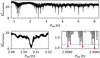 |
Fig. 1 Periodogram for asteroid (7025) 1993 QA. Top panel: normalized χ2 vs. Psid across the tested range of periods with a step size of 0.8∆P. Bottom left: resampled region around the global minimum with steps of 0.1∆P. Bottom right: closer view of the global minimum, revealing aliases caused by long gaps between apparitions. Periods corresponding to local χ2 minima (red dots) below the 3σ threshold (dashed line) were considered for further analysis. |
3.2 Pole and shape
For each period solution within the 3σ confidence limit, we mapped the χ2 values as a function of the asteroid’s spin axis direction, specified in ecliptic coordinates λ and β. Using a modified version of the golden spiral algorithm (Kogan 2017), we generated 30 000 evenly distributed pole directions with an average mutual spacing of approximately 1°. During this step, Psid and the pole coordinates (λ, β) were fixed, and only the shape parameters were optimized.
To estimate the uncertainty of the best-fit pole direction, we again employed the 3σ threshold approach, this time using a higher-degree spherical harmonics model (degree and order six). For cases with nonunique period solutions, we normalized the χ2 values using the lowest global χ2 across all tested periods, creating a spherical map of fit quality in λ and β. To bound the uncertainty of the pole, we then selected only the pole directions from this map with χ2 below the 3σ threshold. An example of such an uncertainty region is shown for asteroid (7025) in Fig. 2. We show the uncertainty regions for individual asteroids in Appendix B. As can be seen in Fig. 2 and the figures in Appendix B, the uncertainty regions have irregular shapes in most cases. To provide a consistent and quantifiable measure of the pole uncertainty for comparison across asteroids, we approximated the uncertainty region as a cone with its apex at the center of the celestial sphere and its base encompassing the region. The radii of these bases are listed in Table A.2.
For each valid Psid solution, we derived the asteroid’s best- fit pole direction and shape model. Not all resulting shapes were physically plausible; some had pole directions deviating significantly from the principal axis of maximum inertia. Following Ďurech et al. (2016), we rejected models where the ratio of the moments of inertia along the shortest principal axis and the rotation axis exceeded 1.1. An example of the final shape model for asteroid (7025) is shown in Fig. 3.
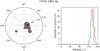 |
Fig. 2 Pole direction and obliquity distribution of (7025) 1993 QA. Left: polar projection of the southern ecliptic hemisphere showing the possible pole directions of asteroid (7025) 1993 QA. The global best-fit pole direction for Psid = 2.506299 h is indicated by the red circle, and the best-fit pole direction for the second-best period the blue circle. The combined 3σ uncertainty region is shaded in gray. Right: histogram of obliquities corresponding to all accepted pole directions within the 3σ uncertainty range, weighted by their respective χ2 values and binned in 5° intervals. The dashed red line represents the obliquity of the nominal pole direction. |
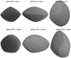 |
Fig. 3 Best-fit convex shape models of the asteroid (7025) 1993 QA. Top row: Psid = 2.506299 h. Bottom row: Psid = 2.506168 h. Left: view along the x-axis (the longest axis) from the asteroid’s equatorial plane. Middle: view along the y-axis from the asteroid’s equatorial plane. Right: view along the z-axis (rotational axis). |
4 Results
In this section, we present the modeling results for individual asteroids. A summary of these results is provided in Table A.2. Comparisons between the observed and synthetic light curves for each model are included in Appendix C.
4.1 (5189) 1990 UQ
Asteroid (5189) 1990 UQ was observed during four apparitions in 2017, 2019, early 2021, and late 2021. We derived a unique solution for the sidereal rotational period, Psid = 6.65738 ± 0.00002 h (all uncertainties are reported at the 3σ level), which agrees with the Psid = 6.657399 h period reported by Warner et al. (2021). The best-fit pole direction for the asteroid is λ ,β = 224°, −85°, with an uncertainty radius of approximately 13°. Our nominal pole solution deviates by about 6° from the best- fit solution reported by Warner et al. (2021). The asteroid is a retrograde rotator, with an obliquity (i.e., the angle between the asteroid’s positive rotational pole direction and the normal to its orbital plane) of є = 179° based on the best-fit pole direction (see Fig. B.1). The derived convex shape model is shown in Fig. B.2. The surface-fit triaxial ellipsoid has axis ratios of a/b = 1.61 and a/c = 2.67, where the c-axis corresponds to the rotational axis.
4.2 (6569) Ondaatje
Observations of asteroid (6569) Ondaatje in its apparitions during 1995, 2010, 2020, and 2022 produced dense light curves. Additionally, sparse photometric data from the ATLAS survey are available for the years 2016, 2018, 2020, and 2022. Notably, the 2010 dataset contains only a single nightly light curve, which exhibits a time offset of approximately 20 minutes compared to our best-fit sidereal period. Attempts to reconcile this offset by adjusting the value of Psid resulted in poor fits to the rest of the observational data. Due to the lack of additional data from 2010, it remains unclear whether this discrepancy arises from an unmodeled feature of the asteroid’s shape, a timing error in the 2010 observations, or the influence of the Yarkovsky-O’Keefe- Radzievskii–Paddack (YORP) effect (see, e.g., Vokrouhlický et al. 2015). Given this uncertainty, we excluded the 2010 light curve from further analysis.
Our analysis yielded a unique solution for the sidereal rotational period Psid = 5.960234 ± 0.000004 h and a best-fit pole orientation at ecliptic coordinates λ, β = 214°, −72° (obliquity є = 173°), with an approximate uncertainty radius of 10° (see Fig. B.3). The convex shape model derived for (6569) Ondaatje is illustrated in Fig. B.4. The surface-fit triaxial ellipsoid has axis ratios of a/b = 1.94 and a/c = 2.02, where the c-axis corresponds to the asteroid’s rotational axis.
4.3 (7025) 1993 QA
We observed asteroid (7025) 1993 QA in 1996 and 2023 and supplemented our dense light curves with sparse data from ATLAS that were acquired in 2020. An initial period search using a simplified shape model (see Sect. 3.1) identified three potential periods (see Fig. 1). Further pole-direction scans eliminated one of the candidate periods, as even the best-fit model for this period exceeded the 3σ threshold established by the globally best-fit solution. The global best solution is Psid = 2.506299 ± 0.000001 h with the pole direction λ,β = 339°, −77° (є = 160°) and axis ratios a/b = 1.27 and a/c = 1.32 of the surface-fit triaxial ellipsoid. For the second-best period, Psid = 2.506168 ± 0.000001 h, the best-fit pole direction is λ,β = 13°, −71° (є = 151°) with the axis ratios of the surface-fit triaxial ellipsoid a/b = 1.10 and a/c = 1.37, where c is also the rotational axis. The two best-fit pole directions for the candidate periods are separated by 5.4°, well within the 3σ uncertainty area, which has an approximate radius of 15° (see Fig. 2). The convex shapes corresponding to the two candidate periods are shown in Fig. 3.
4.4 (8566) 1996 EN
Asteroid (8566) 1996 EN was observed during four apparitions: early 2020, late 2020 (sparse data), early 2022, and late 2022. We determined a unique sidereal period of Psid = 4.8440 ± 0.0001 h. The best-fit pole direction was found to be λ,β = 112°, −84° (є = 137°) with an uncertainty radius of approximately 19° (see Fig. B.5). The convex shape model of (8566) is nearly spherical, with axis ratios of the surface-fit ellipsoid being a/b = 1.03 and a/c = 1.12. The shape is illustrated in Fig. B.6.
4.5 (66251) 1999 GJ2
Asteroid (66251) 1999 GJ2 was observed during four apparitions in 2005, 2007, 2020, and 2022. Despite observations in multiple apparitions, we could not determine a unique period solution. However, we identified 12 potential periods within the 3σ threshold, constraining the sidereal period to  h. One period (Psid = 2.461698 h) was excluded due to the unrealistic rotation of the corresponding best-fit shape model (see Sect. 3.2). The rotational axis of (66251) is primarily constrained to the southern ecliptic hemisphere, though not exclusively (see Fig. B.7). Approximately 98% of the pole directions within the threshold correspond to a retrograde rotation direction. The asteroid’s shape is well constrained in terms of the a/b ratio of the surface-fit ellipsoids, which ranges from 1.01 to 1.09. However, the a /c ratio exhibits greater variability, ranging from 1.07 to 1.49.
4.6 (86450) 2000 CK33
Asteroid (86450) 2000 CK33 was observed in 2005, 2021, and 2022. The dataset was supplemented with ATLAS observations from 2020, 2021, and 2022. We determined a unique sidereal period of Psid = 6.60564 ± 0.00002 h, with a best-fit pole direction of λ,β = 208°, −68° (ϵ = 174°) and an uncertainty radius of approximately 15° (see Fig. B.8). The best-fit shape model indicates an elongated structure, with axis ratios of the surface-fit ellipsoid being a/b = 1.99 and a/c = 2.25 (see Fig. B.9).
4.7 (98943)2001 CC21
Asteroid (98943) 2001 CC21 is a target of the extended Japanese space mission Hayabusa2# (Hirabayashi et al. 2021; Mimasu et al. 2022). While its final target is the small, fast-spinning asteroid 1998 KY26 (scheduled for a rendezvous in 2031), the spacecraft will fly by (98943) in 2026.
We observed (98943) in 2002, 2003, 2022, and 2023. A unique sidereal period of Psid = 5.021522 ± 0.000003 h was determined, along with a well-constrained north pole direction at λ,β = 259°, +84°, with an uncertainty radius of approximately 8° (see Fig. B.10). The obliquity of the best-fit pole direction is ϵ = 7°, indicating a prograde rotator. The derived convex shape model is shown in Fig. B.11, with axis ratios of the surface-fit ellipsoid being a/b = 1.59 and a/c = 2.15.
4.8 (137199) 1999 KX4
Asteroid (137199) 1999 KX4 was observed during four apparitions in 2013, 2019, 2020, and 2022. We determined a unique sidereal period of Psid = 2.769675 ± 0.000008 h. The best-fit pole solution is λ,β = 92°, −60°, with an uncertainty radius of approximately 18°. However, two additional pole directions within the 3σ uncertainty limit were identified: λ,β = 202°, −14° (with an uncertainty radius of 8°) and λ,β = 150°, −35° (with an uncertainty radius of 6°). All pole directions correspond to a retrograde rotation direction for (137199) (see Fig. B.12). The best-fit convex shape model is presented in Fig. B.13, with the surface-fit ellipsoid having axis ratios of a /b = 1.05 and a /c = 1.41.
4.9 (276786) 2004 KD1
Asteroid (276786) 2004 KD1 was sparsely observed in 2013, with dense photometric observations conducted in 2022. Four possible sidereal periods were identified within the 3σ threshold, with the best-fit period being  h. The derived uncertainties also encompass the other three possible periods. Models for two of the four candidate periods were discarded due to their physically unrealistic rotation properties (see Sect. 3.2). For the best-fit period of Psid = 5.018636 ± 0.000003 h, the optimal pole direction was λ,β = 304°, −59°, with an uncertainty region of approximately 22° (ϵ = 153°). The corresponding shape, shown in Fig. B.15 (top panel), has axis ratios of a/b = 1.75 and a/c = 2.03. For the period Psid = 5.0170510 ± 0.000003 h, the best-fit pole direction was λ,β = 202°, +56°, with an uncertainty region radius of approximately 8° (є = 25°). The associated shape, shown in Fig. B.15 (bottom panel), has axis ratios of a/b = 1.20 and a/c = 1.49. Approximately 82% of pole directions within the 3σ threshold correspond to a retrograde rotation direction for (276786) (see Fig. B.14).
4.10 (495615) 2015 PQ291
Asteroid (495615) 2015 PQ291 was observed in 2020 and 2022. Three potential sidereal periods were identified in our periodogram, with the best-fit value being  h. The period Psid = 13.76023 h was excluded as it corresponded to an unrealistic rotation (see Sect. 3.2).For the best-fit period of Psid = 13.7413 ± 0.0007 h, the pole direction was constrained to the northern ecliptic hemisphere, with the global best-fit direction at λ,β = 151°, +45°, and an uncertainty radius of approximately 33° (ϵ = 11°). The surface-fit ellipsoid’s axis ratios were a/b = 1.48 and a/c = 1.58. For the second-best period of Psid = 13.7518 ± 0.0007 h, the optimal pole direction was λ,β = 126°, +33°, with an uncertainty radius of approximately 21° (ϵ = 26°). The axis ratios for this solution were a/b = 1.42 and a/c = 2.16. Figure B.16 displays the best-fit pole directions along with their respective 3σ uncertainty regions. The derived shape models are shown in Fig. B.17.
4.11 (512245) 2016 AU8
Asteroid (512245) 2016 AU8 was observed during five apparitions: early 2018, late 2018/early 2019, 2020, 2021, and 2022. A unique sidereal period of Psid = 4.50541 ± 0.00004 h was determined. The best-fit pole direction was λ,β = 75°, −86° (ϵ = 173°), with an asymmetrical uncertainty region extending up to β~−45° in the direction of λ ~ 320° (see Fig. B.18). The convex shape of (512245) is shown in Fig. B.19. The axis ratios of the surface-fit ellipsoid are a/b = 1.25 and a/c = 2.15.
4.12 Failed cases
(7482) 1994 PC1
Asteroid (7482) 1994 PC1 was observed during two apparitions: in 1997 and again in late 2021 to early 2022. A total of 256 possible rotational periods were identified in our analysis. We were only able to constrain the sidereal period to  h, which remains inconclusive. No further modeling or analysis was conducted for this asteroid.
(22099) 2000 EX106
Asteroid (22099) 2000 EX106 was observed during multiple apparitions in 2000, 2015, early 2022, and late 2022. Additionally, sparse data from the ATLAS survey were available from 2016 and early 2022. Despite these observations, our periodogram revealed 16 local χ2 minima within the 3σ threshold. The nominal best-fit sidereal period was determined to be  h. The best-fit pole directions varied significantly among the candidate periods, as shown in Fig. B.20, and no meaningful constraints on the asteroid’s pole orientation or shape could be derived. The low number of data points per apparition (see Table A.3) is likely a significant factor contributing to the modeling challenges.
(170891) 2004 TY16
Asteroid (170891) 2004 TY16 was observed during two apparitions, in 2008 and 2022. While we constrained the sidereal period to  h, this range includes 78 potential periods within the 3σ threshold of the χ2 periodogram. Consequently, we could not meaningfully determine the pole orientation or rotation direction for this asteroid.
(329437) 2002 OA22
Asteroid (329437) 2002 OA22 was observed during two apparitions, in 2013 and 2022. From our analysis, we identified 12 local minima in the χ2 periodogram and constrained the sidereal rotational period to Psid = 2.6204 ± 0.0009 h.
(506459) 2002 AL14
Asteroid (506459) 2002 AL14 was observed during three apparitions: in 2002, late 2021 to early 2022, and late 2022 to early 2023. Due to the nearly 20-year span of observations, we required a fine time-step resolution in our periodogram analysis. This resulted in 83 closely packed local minima in the χ2 periodogram. The best-fit sidereal period was determined to be  h.However, even for individual candidate periods, the pole direction remained unconstrained, making it impossible to derive a reliable combined pole solution.
2013 BO76
Asteroid 2013 BO76 was observed during two apparitions, in 2013 and 2022. From our analysis, 172 possible sidereal periods were identified. The sidereal period was only loosely constrained to Psid = 5.11 ± 0.01 h, preventing further detailed modeling.
5 Conditions of success
We devote this section to a discussion about circumstances that might have played a role in the success rate of our modeling.
5.1 Phase angle bisector coverage
We tested a hypothesis that one of the key criteria determining the success or failure of our modeling is the range of different viewing circumstances of a given asteroid. Rather than using the asteroid’s ecliptic longitude, we employed the phase angle bisector (PAB), which is the mean direction between the heliocentric and geocentric directions toward the asteroid. As discussed in Harris et al. (1984), this is an approximation for the effective viewing direction of an asteroid observed at the nonzero solar phase. We computed the PAB vector for the mid-point of each light curve run and projected this vector onto the orbital plane of the asteroid. We then computed an oriented angle between this projection and an arbitrary reference direction lying also in the orbital plane. By plotting these angles on a circle, we obtain points corresponding to each light curve session (see Fig. 4). A fraction of the area defined by a polygon made from the session points and the area of the full circle gives us a quantitative estimate of how well a given asteroid was observed for different viewing circumstances. Results discussed further in this section suggest that the PAB coverage is not a robust indicator of the chances of modeling success and that our hypothesis is not valid. However, as discussed further in Sect. 5.2, for unique solutions, PAB coverage appears to correlate with pole uncertainty, with higher coverage corresponding to lower uncertainty.
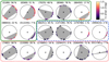 |
Fig. 4 PAB coverage for the studied asteroids, with modeled light curve amplitudes indicated. Asteroids are categorized as follows: well- constrained period and pole direction (solid green line), partially constrained with meaningful period and pole direction (dashed blue line), and cases without reliable solutions (dotted red line). |
5.2 Contribution of sparse data
We found ATLAS sparse photometry for eight of the studied asteroids. We compared results obtained with and without the inclusion of these measurements (following the filter procedure described in Sect. 2.1). For three of the four asteroids with a limited number of possible Psid values – namely, asteroids (6569), (8566), and (86450) – the inclusion of ATLAS data helped resolve ambiguities in rotational period or pole direction, allowing us to achieve a unique solution. For asteroid (7025), the number of possible periods was reduced from four to two. On the other hand, for asteroid (66251), the sparse data did not improve the results, likely due to a combination of their low quality and the asteroid’s very low light curve amplitude. The inclusion of sparse data provided only a modest improvement for asteroids with a large number of period aliases, specifically asteroids (7482), (22099), and (86450).
5.3 Success conditions
Table A.3 summarizes key factors that may influence the success rate of inverse-method modeling. In our dataset, we observe that a dense photometric light curve – one that covers a substantial portion of the asteroid’s revolution in a single night – obtained for a given asteroid in at least two apparitions significantly increases the modeling success rate. Although lower-quality data (with photometric errors ≳0.03 mag) or sparsely sampled light curves still add value by constraining sidereal periods and reducing aliases in periodograms, this is not the case for asteroids with low light curve amplitudes. For such asteroids, a high signal-to-noise ratio is essential for effective modeling.
Of the seven asteroids with fully successful models (well- constrained period and pole direction with physically plausible shape models; see Table A.1), six were observed in at least four apparitions. Asteroid (7025) was observed in only three apparitions, resulting in an ambiguous sidereal period; however, its pole direction is well-constrained and relatively insensitive to the specific period, likely due to the high density of light curves in two of its apparitions. For the four asteroids with the highest observed light curve amplitudes (≥1.1 mag), we successfully constructed unique models. Pole uncertainty generally appears inversely proportional to PAB coverage, with one exception: asteroid (8566), which has the highest PAB coverage at 78% yet the largest pole uncertainty (~ 19°), likely due to its low observed amplitude.
In the partially successful group of the Table A.3, two of the four asteroids were observed in only two apparitions, leading to low PAB coverage. Nevertheless, we managed to reasonably constrain their periods and poles, likely due to their relatively high light curve amplitudes (~1 mag). The other two asteroids in this group, despite being observed in four apparitions, have ambiguous period or pole estimates. Both exhibit relatively short rotational periods (2.5 and 2.8 hours), which may contribute to the ambiguity. In addition, asteroid (66251), one of the shortperiod asteroids, has the lowest light curve amplitude in our sample (~0.25 mag), which may further hinder unique model construction.
For the six asteroids in the failed group of the Table A.3, unsuccessful modeling appears to result from a combination of low light curve amplitudes (all ≲0.6 mag), relatively short rotational periods (four with periods ≲2.8 hours), and long gaps between apparitions. PAB coverage does not seem to impact this group; for example, despite high PAB coverage (72%) and three apparitions for asteroid (506459), the combination of relatively short (0.7-year) and very long (19.5-year) gaps between observations, along with a short rotational period of ~2.3 hours, precludes a unique sidereal period determination, yielding 83 possible periods. Based on the successful models, long gaps between some apparitions appear manageable if data from a closer, but not too close, apparition are also available — an interval of approximately two years seems ideal. Of course, this optimal interval may vary depending on the asteroid’s rotational period (with longer periods tolerating longer gaps) and the precision with which the period can be estimated from individual apparitions, which in turn depends on the data quality and density.
5.4 Summary
From our sample of 17 NEAs, we found that long gaps between some apparitions can be valuable for constraining the sidereal period of an asteroid, provided that additional data from a closer apparition are available. A gap of approximately two years appears optimal for uniquely linking recent observations with archival data taken decades earlier. However, as noted in Marciniak et al. (2015, 2018), small light curve amplitudes can complicate period determination, as seen with asteroid (66251) in Table A.3. Asteroids with rotational periods between 4 and 7 hours seem ideal for modeling, as this range allows for substantial light curve coverage in a single night while still meeting the precision requirements for linking distant apparitions. For asteroids with shorter periods (<3 hours), light curves are generally well-covered, though the period itself is often ambiguous. While linking a distant apparition for long-period asteroids is easier, only a portion of the full light curve can be observed in one night, and aliases with the Earth’s 24-hour rotation cycle can prevent full coverage within a single lunation (resulting in repeated observation of the same part of the light curve each night).
Densely sampled observations covering a large portion of the light curve, observed from at least two distinct viewing geometries – typically across different apparitions – are essential for reliable pole constraint, as demonstrated by asteroid (7025) in Table A.3. Sparse data help constrain the period and primarily aid in uniquely linking distant observations. However, our hypothesis that PAB coverage would indicate modeling success was not confirmed.
6 Conclusions
Between 2020 and 2023, we conducted photometric observations of 17 selected NEAs with available archival data. This enabled us to attempt rotational state and shape estimation. For 6 of the 17 asteroids, we were unable to reliably constrain their sidereal rotational periods due to multiple closely spaced alias periods, largely resulting from extensive gaps between their apparitions. For 7 of the asteroids, we determined the pole direction with an approximate uncertainty radius of ≲20° and derived convex shape models. For the remaining 4 asteroids, we managed to constrain their sidereal periods and pole directions to varying degrees of accuracy and estimated their possible shapes for each plausible period. Notably, when multiple period solutions exist, pole direction estimates tend to be ambiguous; however, once a unique period is established, the ambiguity in pole direction is typically resolved.
We further explored the limitations of the asteroid light curve inversion method and the impact of long observational gaps in our dataset. For asteroids with rotational periods ≳3 h, an observation interval of approximately two years between apparitions appears optimal for achieving unique sidereal period determinations, especially when combined with data from decades-old observations. While close period aliases were common (and suppressed in some cases by sparse ATLAS data), we were often able to constrain the asteroid’s pole direction or its rotation direction if the number of aliases was not excessive. For instance, asteroid (66251) is very likely a retrograde rotator, despite having 11 possible sidereal period values. We confirmed that high-amplitude asteroids are more likely to yield successful models, and that dense photometric light curves from at least two apparitions for a given asteroid significantly enhance the chances of finding a unique solution. In contrast, PAB coverage appears to play a relatively minor role in obtaining accurate period estimates compared to other factors.
Data availability
Appendices A, B, and C can be accessed at the permanent URL https://doi.org/10.5281/zenodo.14773077.
All observational tables, lightcurve data and models are available at the CDS via anonymous ftp to cdsarc.cds.unistra.fr (130.79.128.5) or via https://cdsarc.cds.unistra.fr/viz-bin/cat/J/A+A/695/A139
Acknowledgements
We thank S. Rahvar and S. Sajadian for their observations performed as part of the MiNDSTEp team. We sincerely thank the anonymous referee for their constructive comments and insightful suggestions, which greatly improved the quality of this manuscript. We acknowledge funding from the European Union’s Horizon 2020 research and innovation programme under grant agreement No. 870403. Computational resources were provided by the e-INFRA CZ project (ID:90254), supported by the Ministry of Education, Youth and Sports of the Czech Republic. N. P. acknowledges funding by Fundação para a Ciência e a Tecnologia (FCT) through the research grants UIDB/04434/2020 and UIDP/04434/2020. We thank Uffe Gråe Jørgensen and Martin Dominik for the management and time allocation of the MiNDSTEp observation of NEAs. All observations carried out at the MAO supported by the basic governmental funding of the Laboratory of Galactic Astronomy of the UBAI. The work at Modra was supported by the Slovak Grant Agency for Science VEGA, Grant 1/0530/22. The work at the McDonald observatory was funded by NASA’s NEO Observation Program Grants NAG5-10183 and NAG5-13302. This work uses data from the University of Hawaii’s ATLAS project, funded through NASA grants NN12AR55G, 80NSSC18K0284, and 80NSSC18K1575, with contributions from the Queen’s University Belfast, STScI, the South African Astronomical Observatory, and the Millennium Institute of Astrophysics, Chile. We used the publicly available code for the sidereal period search and the light curve inversion6 written by Josef Durech (which is based on Kaasalainen & Torppa 2001; Kaasalainen et al. 2001). In this work we made extensive use of the programming language Python 3 (Van Rossum & Drake 2009) and its non-standard libraries NumPy (Harris et al. 2020), SciPy (Virtanen et al. 2020), Matplotlib (Hunter 2007), and Astropy (Astropy Collaboration 2013, 2018, 2022). Some of the photometric data were reduced with the MPO Canopus software (Warner 2012). We acknowledge the use of OpenAI’s ChatGPT for assistance with language refinement and editing of the manuscript.
Appendix A Tables
Observational circumstances of the studied asteroids.
Overview of the modeling results.
Asteroid observation circumstances and success rate in modeling.
References
- Astropy Collaboration (Robitaille, T. P., et al.) 2013, A&A, 558, A33 [NASA ADS] [CrossRef] [EDP Sciences] [Google Scholar]
- Astropy Collaboration (Price-Whelan, A. M., et al.) 2018, AJ, 156, 123 [Google Scholar]
- Astropy Collaboration (Price-Whelan, A. M., et al.) 2022, ApJ, 935, 167 [NASA ADS] [CrossRef] [Google Scholar]
- Azimov, A. M., Tillayev, Y. A., Ehgamberdiev, S. A., & Ilyasov, S. P. 2022, J. Astron. Telesc. Instrum. Syst., 8, 047002 [NASA ADS] [CrossRef] [Google Scholar]
- Bartczak, P., & Dudzinski, G. 2018, MNRAS, 473, 5050 [NASA ADS] [CrossRef] [Google Scholar]
- Benishek, V. 2021, Minor Planet Bull., 48, 77 [NASA ADS] [Google Scholar]
- Carbognani, A. 2008, Minor Planet Bull., 35, 109 [NASA ADS] [Google Scholar]
- Carbognani, A. 2014, Minor Planet Bull., 41, 4 [NASA ADS] [Google Scholar]
- Cheng, A. F., Rivkin, A. S., Michel, P., et al. 2018, Planet. Space Sci., 157, 104 [CrossRef] [Google Scholar]
- Daly, R. T., Ernst, C. M., Barnouin, O. S., et al. 2023, Nature, 616, 443 [CrossRef] [Google Scholar]
- Dotto, E., Banaszkiewicz, M., Banchi, S., et al. 2021, in 7th IAA Planetary Defense Conference, 221 [Google Scholar]
- Durech, J., Sidorin, V., & Kaasalainen, M. 2010, A&A, 513, A46 [NASA ADS] [CrossRef] [EDP Sciences] [Google Scholar]
- Ďurech, J., Hanuš, J., Oszkiewicz, D., & Vančo, R. 2016, A&A, 587, A48 [NASA ADS] [CrossRef] [EDP Sciences] [Google Scholar]
- Ehgamberdiev, S. 2018, Nat. Astron., 2, 349 [NASA ADS] [CrossRef] [Google Scholar]
- Franco, L., Marchini, A., Papini, R., et al. 2022, Minor Planet Bull., 49, 200 [NASA ADS] [Google Scholar]
- Harris, A. W., Young, J. W., Scaltriti, F., & Zappala, V. 1984, Icarus, 57, 251 [NASA ADS] [CrossRef] [Google Scholar]
- Harris, C. R., Millman, K. J., van der Walt, S. J., et al. 2020, Nature, 585, 357 [NASA ADS] [CrossRef] [Google Scholar]
- Hirabayashi, M., Mimasu, Y., Sakatani, N., et al. 2021, Adv. Space Res., 68, 1533 [NASA ADS] [CrossRef] [Google Scholar]
- Hunter, J. D. 2007, Comput. Sci. Eng., 9, 90 [NASA ADS] [CrossRef] [Google Scholar]
- Im, M.-S., Ko, J.-W., Cho, Y.-S., et al. 2010, J. Korean Astron. Soc., 43, 75 [NASA ADS] [CrossRef] [Google Scholar]
- Kaasalainen, M. 2004, A&A, 422, L39 [NASA ADS] [CrossRef] [EDP Sciences] [Google Scholar]
- Kaasalainen, M., & Torppa, J. 2001, Icarus, 153, 24 [NASA ADS] [CrossRef] [Google Scholar]
- Kaasalainen, M., Torppa, J., & Muinonen, K. 2001, Icarus, 153, 37 [NASA ADS] [CrossRef] [Google Scholar]
- Kaiser, N., Aussel, H., Burke, B. E., et al. 2002, SPIE Conf. Ser., 4836, 154 [Google Scholar]
- Kaiser, N., Burgett, W., Chambers, K., et al. 2010, SPIE Conf. Ser., 7733, 77330E [Google Scholar]
- Kogan, J. 2017, Rose–Hulman Undergrad. Math. J., 18 [Google Scholar]
- Krugly, Y. N., Belskaya, I. N., Shevchenko, V. G., et al. 2002, Icarus, 158, 294 [NASA ADS] [CrossRef] [Google Scholar]
- Landolt, A. U. 1992, AJ, 104, 340 [Google Scholar]
- Lauretta, D. S., Balram-Knutson, S. S., Beshore, E., et al. 2017, Space Sci. Rev., 212, 925 [Google Scholar]
- Marciniak, A., Pilcher, F., Oszkiewicz, D., et al. 2015, Planet. Space Sci., 118, 256 [NASA ADS] [CrossRef] [Google Scholar]
- Marciniak, A., Bartczak, P., Müller, T., et al. 2018, A&A, 610, A7 [NASA ADS] [CrossRef] [EDP Sciences] [Google Scholar]
- McMillan, R. S., Bressi, T. H., Scotti, J. V., Larsen, J. A., & Perry, M. L. 2012, in AAS/Division for Planetary Sciences Meeting Abstracts, 44, 210.14 [Google Scholar]
- Mimasu, Y., Kikuchi, S., Takei, Y., et al. 2022, in Hayabusa2 Asteroid Sample Return Mission, eds. M. Hirabayashi & Y. Tsuda (Elsevier), 557 [CrossRef] [Google Scholar]
- Oey, J. 2020, Minor Planet Bull., 47, 136 [NASA ADS] [Google Scholar]
- Ostro, S. J., Connelly, R., & Belkora, L. 1988, Icarus, 73, 15 [NASA ADS] [CrossRef] [Google Scholar]
- Polishook, D. 2012, Minor Planet Bull., 39, 187 [NASA ADS] [Google Scholar]
- Polishook, D., & Brosch, N. 2008, Icarus, 194, 111 [Google Scholar]
- Pravec, P., Šarounová, L., & Wolf, M. 1996, Icarus, 124, 471 [NASA ADS] [CrossRef] [Google Scholar]
- Pravec, P., Wolf, M., & Šarounová, L. 1998, Icarus, 136, 124 [NASA ADS] [CrossRef] [Google Scholar]
- Press, W. H., Teukolsky, S. A., Vetterling, W. T., & Flannery, B. P. 2007, Numerical Recipes: The Art of Scientific Computing, 3rd edn. (USA: Cambridge University Press) [Google Scholar]
- Ries, J. G., & Varadi, F. 2007, in AAS/Division for Planetary Sciences Meeting Abstracts, 39, 35.16 [Google Scholar]
- Rivkin, A. S., Chabot, N. L., Stickle, A. M., et al. 2021, Planet. Sci. J., 2, 173 [NASA ADS] [CrossRef] [Google Scholar]
- Schmalz, S., Schmalz, A., Voropaev, V., et al. 2023, Minor Planet Bull., 50, 43 [NASA ADS] [Google Scholar]
- Stokes, G. H., Evans, J. B., Viggh, H. E. M., Shelly, F. C., & Pearce, E. C. 2000, Icarus, 148, 21 [NASA ADS] [CrossRef] [Google Scholar]
- Thirouin, A., Moskovitz, N., Binzel, R. P., et al. 2016, AJ, 152, 163 [NASA ADS] [CrossRef] [Google Scholar]
- Tonry, J. L., Denneau, L., Heinze, A. N., et al. 2018, PASP, 130, 064505 [Google Scholar]
- Tsuda, Y., Yoshikawa, M., Abe, M., Minamino, H., & Nakazawa, S. 2013, Acta Astronautica, 91, 356 [CrossRef] [Google Scholar]
- Vaduvescu, O., Aznar Macias, A., Wilson, T. G., et al. 2022, Earth Moon Planets, 126, 6 [NASA ADS] [CrossRef] [Google Scholar]
- Van Rossum, G., & Drake, F. L. 2009, Python 3 Reference Manual (Scotts Valley, CA: CreateSpace) [Google Scholar]
- Viikinkoski, M., Kaasalainen, M., & Durech, J. 2015, A&A, 576, A8 [NASA ADS] [CrossRef] [EDP Sciences] [Google Scholar]
- Viikinkoski, M., Hanuš, J., Kaasalainen, M., Marchis, F., & Durech, J. 2017, A&A, 607, A117 [NASA ADS] [CrossRef] [EDP Sciences] [Google Scholar]
- Virtanen, P., Gommers, R., Oliphant, T. E., et al. 2020, Nat. Methods, 17, 261 [Google Scholar]
- Vokrouhlický, D., Bottke, W. F., Chesley, S. R., Scheeres, D. J., & Statler, T. S. 2015, in Asteroids IV, 509 [Google Scholar]
- Warner, B. D. 2012, MPO Canopus version 10, Bdw Publishing, Eaton, CO, USA [Google Scholar]
- Warner, B. D. 2013, Minor Planet Bull., 40, 137 [NASA ADS] [Google Scholar]
- Warner, B. D. 2014, Minor Planet Bull., 41, 41 [NASA ADS] [Google Scholar]
- Warner, B. D. 2015, Minor Planet Bull., 42, 172 [NASA ADS] [Google Scholar]
- Warner, B. D. 2018, Minor Planet Bull., 45, 138 [NASA ADS] [Google Scholar]
- Warner, B. D., & Stephens, R. D. 2019a, Minor Planet Bull., 46, 144 [NASA ADS] [Google Scholar]
- Warner, B. D., & Stephens, R. D. 2019b, Minor Planet Bull., 46, 304 [Google Scholar]
- Warner, B. D., & Stephens, R. D. 2020a, Minor Planet Bul., 47, 200 [NASA ADS] [Google Scholar]
- Warner, B. D., & Stephens, R. D. 2020b, Minor Planet Bull., 47, 105 [NASA ADS] [Google Scholar]
- Warner, B. D., & Stephens, R. D. 2020c, Minor Planet Bull., 47, 290 [NASA ADS] [Google Scholar]
- Warner, B. D., & Stephens, R. D. 2022a, Minor Planet Bull., 49, 176 [NASA ADS] [Google Scholar]
- Warner, B. D., & Stephens, R. D. 2022b, Minor Planet Bull., 49, 274 [NASA ADS] [Google Scholar]
- Warner, B. D., Stephens, R. D., & Harris, A. W. 2011, Minor Planet Bull., 38, 172 [NASA ADS] [Google Scholar]
- Warner, B. D., Stephens, R. D., & Coley, D. R. 2021, Minor Planet Bull., 48, 337 [NASA ADS] [Google Scholar]
- Waszczak, A., Chang, C.-K., Ofek, E. O., et al. 2015, AJ, 150, 75 [NASA ADS] [CrossRef] [Google Scholar]
- Watanabe, S.-I., Tsuda, Y., Yoshikawa, M., et al. 2017, Space Sci. Rev., 208, 3 [NASA ADS] [CrossRef] [Google Scholar]
- Watanabe, S., Hirabayashi, M., Hirata, N., et al. 2019, Science, 364, 268 [NASA ADS] [Google Scholar]
NEOROCKS was funded by the European Union’s Horizon 2020 research and innovation program. One of its goals was the physical characterization of NEAs through photometric observations.
See their Sects. 6.14.8 and 15.1.1.
Degrees of freedom = number of data points - number of free parameters.
All Tables
All Figures
|
Fig. 1 Periodogram for asteroid (7025) 1993 QA. Top panel: normalized χ2 vs. Psid across the tested range of periods with a step size of 0.8∆P. Bottom left: resampled region around the global minimum with steps of 0.1∆P. Bottom right: closer view of the global minimum, revealing aliases caused by long gaps between apparitions. Periods corresponding to local χ2 minima (red dots) below the 3σ threshold (dashed line) were considered for further analysis. |
| In the text | |
|
Fig. 2 Pole direction and obliquity distribution of (7025) 1993 QA. Left: polar projection of the southern ecliptic hemisphere showing the possible pole directions of asteroid (7025) 1993 QA. The global best-fit pole direction for Psid = 2.506299 h is indicated by the red circle, and the best-fit pole direction for the second-best period the blue circle. The combined 3σ uncertainty region is shaded in gray. Right: histogram of obliquities corresponding to all accepted pole directions within the 3σ uncertainty range, weighted by their respective χ2 values and binned in 5° intervals. The dashed red line represents the obliquity of the nominal pole direction. |
| In the text | |
|
Fig. 3 Best-fit convex shape models of the asteroid (7025) 1993 QA. Top row: Psid = 2.506299 h. Bottom row: Psid = 2.506168 h. Left: view along the x-axis (the longest axis) from the asteroid’s equatorial plane. Middle: view along the y-axis from the asteroid’s equatorial plane. Right: view along the z-axis (rotational axis). |
| In the text | |
|
Fig. 4 PAB coverage for the studied asteroids, with modeled light curve amplitudes indicated. Asteroids are categorized as follows: well- constrained period and pole direction (solid green line), partially constrained with meaningful period and pole direction (dashed blue line), and cases without reliable solutions (dotted red line). |
| In the text | |
Current usage metrics show cumulative count of Article Views (full-text article views including HTML views, PDF and ePub downloads, according to the available data) and Abstracts Views on Vision4Press platform.
Data correspond to usage on the plateform after 2015. The current usage metrics is available 48-96 hours after online publication and is updated daily on week days.
Initial download of the metrics may take a while.