| Issue |
A&A
Volume 694, February 2025
|
|
|---|---|---|
| Article Number | A118 | |
| Number of page(s) | 8 | |
| Section | Extragalactic astronomy | |
| DOI | https://doi.org/10.1051/0004-6361/202452586 | |
| Published online | 07 February 2025 | |
An accurate and simple asymptotically matched deprojection of the Sérsic law
1
Department of Physics and Astronomy, University of Bologna, Via Gobetti 93/2, 40129 Bologna, Italy
2
INAF – Osservatorio di Astrofisica e Scienza dello Spazio di Bologna, Via Gobetti 93/3, 40129 Bologna, Italy
3
International PhD College – Collegio Superiore, University of Bologna, Bologna, Italy
⋆ Corresponding author; This email address is being protected from spambots. You need JavaScript enabled to view it.
Received:
11
October
2024
Accepted:
2
January
2025
Abstract
Context. The Sérsic law reproduces very well the surface brightness profile of early-type galaxies, and therefore it is routinely used in observational and theoretical works. Unfortunately, its deprojection cannot be expressed in terms of elementary functions for generic values of the shape parameter n. Over the years, different families of approximate deprojection formulae have been proposed, generally based on fits of the numerical deprojection over some radial range.
Aims. We searched for a very simple, accurate, and theoretically motivated deprojection formula of the Sérsic law without free parameters, not based on fits of the numerical deprojection, and holding for generic n > 1.
Methods. We found the formula by requiring it to reproduce the analytical expressions for the inner and outer asymptotic expansions of the deprojected Sérsic law of a given n and by matching the two expansions at intermediate radii with the request that the total luminosity coincides with that of the original Sérsic profile of the same n.
Results. The resulting formula is algebraically very simple. By construction, its inner and outer parts are the exact (asymptotic) deprojection of the Sérsic law, and it depends on two coefficients that are analytical functions of the n of immediate evaluation. The accuracy of the formula over the whole radial range is very good and increases for increasing n, with a maximum of relative deviations from the true numerical deprojection of ≃8 10−3 for the de Vaucouleurs profile. In the appendix, the extension of the proposed formula to profiles with n < 1 is also presented and discussed.
Conclusions. The formula we obtained is a simple and useful tool that can be used in the modeling of early-type galaxies, and its ellipsoidal generalization is immediate.
Key words: galaxies: elliptical and lenticular / cD / galaxies: structure
© The Authors 2025
 Open Access article, published by EDP Sciences, under the terms of the Creative Commons Attribution License (https://creativecommons.org/licenses/by/4.0), which permits unrestricted use, distribution, and reproduction in any medium, provided the original work is properly cited.
This article is published in open access under the Subscribe to Open model. This email address is being protected from spambots. You need JavaScript enabled to view it. to support open access publication.
1. Introduction
The surface brightness profiles of early-type galaxies are described quite well by the empirical Sérsic (1968) law (e.g., Caon et al. 1993), which is a generalization of the de Vaucouleurs (1948) profile. The Sérsic law has also been used to model dwarf galaxies (e.g., Graham & Guzman 2003; Battaglia et al. 2006), the bulges of spiral galaxies (Andredakis et al. 1995), and globular clusters (e.g., Barmby et al. 2007). For this reason, the Sérsic profile has been used intensively in observational works and has also been investigated in depth from the theoretical point of view (e.g., see Graham & Driver 2005, and references therein). In the following we restrict our discussion to the spherically symmetric case for simplicity, but the generalization to the ellipsoidal case is not difficult (see Section 4; see also Chapter 11 in Ciotti 2021, hereafter C21). The Sérsic profile of spherical galaxies can be written as
 (1)
(1)
where n is the shape parameter, I0 is the central surface brightness, R is the radius in the projection plane, Re is the effective radius (i.e. the radius in the projection plane enclosing half of the total luminosity of the profile), and b is a dimensionless parameter depending on n. The total luminosity associated with the profile in Eq. (1) is
 (2)
(2)
where Γ(x) is the Euler gamma function. Usually, the equation above is used to eliminate I0 in Eq. (1) in favor of L. As is well known the value of the parameter b in Eq. (1) depends on n via the transcendental equation Γ(2n)/2 = γ(2n, b), where γ(a, x) is the lower incomplete gamma function; the equation comes from the request that Re is the effective radius, and since b(n) cannot be expressed in terms of elementary functions, several high-quality fits of the numerical solution have been presented in the literature (see, e.g., Ciotti & Bertin 1999; also see C21). Finally, Ciotti & Bertin (1999) showed that b(n) for n → ∞ can be expressed as the asymptotic series
 (3)
(3)
where higher order terms can be easily constructed. For practical purposes, it should be noticed that the relative error (in absolute value) of Eq. (3) truncated just to the first four terms compared to the true solution for 1 ≤ n ≤ 10 is already as small as ≃3.8 × 10⁻⁶ in the worst n ≃ 1.2 case, decreasing down to ≈10−8 for increasing n. Even for n as low as 1/2, the relative error is ≃7 × 10⁻⁴.
The deprojected luminosity density profile ν(r) of the Sérsic law, which is the focus of the present paper, is given by the usual Abel deprojection integral (e.g., Binney & Tremaine 2008, C21)
 (4)
(4)
where r is the spherical radius. As is well known, ν(r) cannot be expressed in terms of elementary functions for generic values of n. For this reason, a great effort has been devoted to build sufficiently accurate and manageable analytical approximations of the true (i.e., numerical) ν(r), usually valid over some more or less extended radial interval. We mention here a few of the main adopted approaches with a list that is almost certainly not complete:
-
Purely numerical deprojections: The ν(r) profiles are given as tables, in particular for the special case of the de Vaucouleurs n = 4 law (Poveda et al. 1960; Young 1976).
-
Multi-Gaussian deprojections: The ν(r) profiles are determined from the property that the deprojection of a centered Gaussian is a Gaussian. The weights and dispersions of the Gaussian components adopted to expand I(R) in Eq. (1) are determined numerically and given in tables. This approach was used for the n = 4 profile by Bendinelli et al. (1993) and successively extended to generic Sérsic profiles (e.g., Pechetti et al. 2020).
-
Single slope power-law fits: In this important family, ν(r) is approximated as
![Mathematical equation: $$ \begin{aligned} \nu (r)={L\over R_{\rm {e}}^3}{b^{(3-\beta )n}\over 4\pi n\,\Gamma [(3-\beta )n]}s^{-\beta }\mathrm{e}^{-b\, s^{1/n}},\quad s\equiv {r\over R_{\rm {e}}}, \end{aligned} $$](/articles/aa/full_html/2025/02/aa52586-24/aa52586-24-eq5.gif) (5)
(5)(Mellier & Mathez 1987; Prugniel & Simien 1997, see also Gerbal & Lima 1997, Lima 1999; Márquez & Lima 2000; Terzić & Graham 2005). The expression for ν(r) in Eq. (5) guarantees that for generic β < 3, its total luminosity L is the same as that of the Sérsic profile of index n, effective radius Re, and central surface brightness I0. The parameter β is a function of n and is obtained from a fit of the numerically deprojected profile over some prescribed radial range. In this way the value of β also depends on the radial range used for the fit. We notice that Re is the effective radius of the true profile and not that of the deprojected approximated formula (even though they can almost be identical).
-
Refined single slope power-law fits: In this approach, ν(r) is reproduced with modifications of the single power-law fits by considering more complicated functions than the exponential term in Eq. (5), for example, as a sum of exponentials (Simonneau & Prada 2004). In this family we mention the very high-accuracy deprojected profile of Vitral & Mamon (2020), which is obtained by fitting the residuals of Eq. (5) with respect to the true profile with bivariate polynomials of order ten in terms of logi(s)logj(n). The polynomials’ coefficients are given in numerical tables, and the lower limit of the range of r/Re was set to 10−3. In Vitral & Mamon (2021), the lower limit was further reduced to 10−4.
-
Special functions fits: A high-quality fit of ν(r) in terms of the modified Bessel functions of the second kind Kν, supplemented by tables for the numerical values of the parameters as a function of n, is given in Trujillo et al. (2002). A refinement of the formula is given in Emsellem & van de Ven (2008).
-
Analytical deprojections: ν(r) is a Gaussian for n = 1/2, and a modified Bessel function of the second kind K0 for the exponential case n = 1 (e.g., see Baes & Ciotti 2019). Moreover, ν(r) can be expressed in terms of Meijer G functions for all rational values of n (Mazure & Capelato 2002) and in terms of Fox H functions for generic n (Baes & Gentile 2011; Baes & Van Hese 2011). However, these advanced transcendental functions are rarely used in common applications, and they are not routinely implemented in numerical packages. In this family of analytically exact formulae, we also mention those based on the method of asymptotic expansion (Ciotti 1991, hereafter C91; see also C21) that give the asymptotic formulae for ν(r) for r → 0 and for r → ∞. As shown in Section 2, these formulae are the starting point of the present study.
Nowadays, available computer algebra systems allow one to numerically integrate Eq. (4) with arbitrarily large numerical precision so that the need for sophisticated analytical approximations of ν(r) is not as compelling as it was when the de Vaucouleurs and Sérsic laws were introduced. However, an analytical approximation of ν(r) can still be useful if it satisfies the following properties:
(P1) Correct analytical behavior at the center and at large radii. In fact, one of the common uses of an analytical ν(r) is to obtain the radial trends of dynamical quantities (such as, gravitational potential and solutions of Jeans equations) near the center also in presence of a central supermassive black hole. Quite often the approximations of ν(r), obtained as fits over some finite radial range, are not correct at the center and/or at large radii (unless the correct trend is imposed to the functional form of the fitting function).
(P2) Monotonically decreasing behavior for increasing r. This property of the Sérsic law for n ≥ 1/2 follows from the identity
![Mathematical equation: $$ \begin{aligned} {d\,\nu (r)\over dr}=-{r\over \pi }\int _r^{\infty }{d\over dR}\left[{1\over R}{d I(R)\over dR}\right]{dR\over \sqrt{R^2-r^2}}, \end{aligned} $$](/articles/aa/full_html/2025/02/aa52586-24/aa52586-24-eq6.gif) (6)
(6)
which is established with integration by parts of Eq. (4) and then by differentiation with respect to r. For n ≥ 1/2, it is easy to show that the integrand is nowhere negative, while for 0 < n < 1/2, an asymptotic analysis shows that the profile is non-monotonic, with d ν(r)/dr > 0 near the center and negative at large radii.
(P3) Conservation of the total luminosity. The proposed formula should have the same L as the true Sérsic profile of a given n, Re, and I0. It should be noted that in general the Re appearing in the approximate formulae is the effective radius of the true profile, not the effective radius of the approximated formula (even though the two values are of course very similar for high accuracy formulae).
(P4) Accuracy over a large or total radial range. The request is obvious; however, for practical purposes differences of less than a few percent from the true ν(r) can be safely ignored in almost all observational and theoretical works.
(P5) Simplicity. As stated previously, since fast numerical deprojection with arbitrarily high accuracy is now possible, only sufficiently simple formulae can really be useful in applications.
The different formulae proposed so far satisfy some of the properties above, while they are less satisfactory for some others. Here, we follow a different approach from that of previous works, namely, we do not use any fit, but we build a formula starting from the analytically exact (asymptotic) deprojection of the Sérsic law for large and small radii, restricting to n > 1, the range of interest in applications. In this way, the proposed deprojection formula is correct by design for r → 0 and r → ∞. Then we match the two regimes by introducing a transition parameter p whose value is uniquely determined by n and by the request that the total luminosity coincides with L of the original Sérsic law. The resulting formula is extremely simple and performs extremely well over the entire radial range, with relative errors of the order of 10−3 or less (with accuracy improving with increasing n).
The paper is organized as follows: In Section 2, we construct and discuss the proposed deprojection formula, and in Section 3 the formula is compared to the true numerically deprojected Sérsic profile. In Section 4, the main results are summarized.
2. The asymptotically matched deprojection formula
In our study, we mainly focus on the deprojection ν(r) of the Sérsic profile for n > 1, the range encompassing the vast majority of cases of interest for early-type galaxies. In Appendix A, however, we consider in some detail the approximation of ν also for n < 1 profiles. We do not consider the approximation of the deprojection of the n = 1 profile because for this model, ν can be written as a Bessel K0 function:
 (7)
(7)
where s = r/Re, the convention adopted throughout the paper, and b = b(1)≃1.67835. For future reference, we recall that near the origin
 (8)
(8)
where γ ≃ 0.57721 is the Euler constant, and the characteristic central logarithmic divergence of the deprojected exponential profile is apparent (see, e.g., Eq. (A.6) in C91, and Eqs. (8.447.3) and (8.447.1) in Gradshteyn & Ryzhik 2007).
As shown in C91, for 0 < n < 1 near the origin, ν(r) converges to a finite value (dependent on n) as
 (9)
(9)
For n > 1 instead, ν(r) near the origin diverges as1
 (10)
(10)
where B(x, y) is the Euler beta function. In the external regions, the leading term of the asymptotic expansion of ν(r) for a generic n > 0 is finally given by
 (11)
(11)
Of course, in Eqs. (7)–(11), I0 can be expressed in terms of L and Re using Eq. (2).
These asymptotic expansions show that Eq. (5) cannot be simultaneously correct at the center and in the external regions; therefore, single power-law fits cannot be used to evaluate (rigorously) the dynamical properties of ν(r). However, the asymptotic expansions also explain why, after all, the single slope power-law fits in Eq. (5) perform surprisingly well, with increasing accuracy for increasing n. In fact the algebraic factors in Eqs. (10)–(11) behave as r1/n − 1 at the center and as r1/(2n)−1 at large radii so that for n large enough, the two exponents tend to the common limit of −1. For example, for n = 4, the inner and outer power-law exponents are already quite similar: −0.75 at the center and −0.875 in the external regions (in the Mellier & Mathez 1987 formula the best-fit exponent is ≃ − 0.855). We also notice how the asymptotic expansion is not uniform in terms of n; that is, the central behavior of ν for n = 1 cannot be obtained as the limit for n → 1+ of Eq. (10). It is to be expected that for n near unity, the deprojection fomulae based on Eqs. (10)–(11) will be (slightly) less accurate than for (say) n ≥ 2.
Thanks to Eqs. (10)–(11), we can proceed to the construction of a high-accuracy approximated deprojected Sérsic profile that is not a fit, has no free parameters, is monotonically decreasing, and has the same total luminosity and the same exact trend in the internal and external regions as the true deprojected profile. The idea is to exploit the fact that for n > 1, the ratio  is a monotonically increasing function that vanishes at the origin and diverges for r → ∞. This allows us to satisfy all the mentioned requirements (except the conservation of L, which we discuss later) with the elementary trial function
 (12)
(12)
We note that the request of exact central and external behaviors (i.e., that  and
and  ) implies that the coefficients in front of νi(r) and νe(r) in Eq. (12) must be unity, as must also be unity the additive constant in its denominator. We also note that the proposed νa approaches both νi and νe from below.
Of course, νa(r) cannot be expected to describe well the true profile in the intermediate radial region. For example, the volume integration of νa(r) gives a total luminosity that underestimates L of the associated Sérsic profile by ≃19% for n = 2, ≃24% for n = 4, and ≃27% for n = 10. As a consequence, while preserving all its positive features, we must modify Eq. (12) so that its total luminosity coincides with L. The idea is to introduce a matching parameter p (dependent on n) to be uniquely determined by the conservation of L. The most natural choice is to modify Eq. (12) as
![Mathematical equation: $$ \begin{aligned} \nu _{\rm a}(r) = \displaystyle {\nu _{\rm {i}}(r)\over \left\{ 1 +\left[\nu _{\rm {i}}(r)/\nu _{\rm {e}}(r)\right]^p\right\} ^{1/p}} ={L\over R_{\rm {e}}^3}{c_1\,\mathrm{e}^{-b\, s^{1/n}}\over \left[1 + c_2^p\, s^{p/(2n)}\right]^{1/p}s^{1-1/n}}, \end{aligned} $$](/articles/aa/full_html/2025/02/aa52586-24/aa52586-24-eq16.gif) (13)
(13)
where b is again given in Eq. (3), the second formula is expressed in terms of L and Re of the true Sérsic profile, and from Eqs. (10)–(11) the two coefficients are the analytical functions
 (14)
(14)
For p > 0, the asymptotic properties of Eq. (12) are retained, in agreement with the requests in P1, P2, P5 in the Introduction. Moreover, for p > 1 it follows that 1 + x ≥ (1 + xp)1/p∀x ≥ 0 (while the inequality inverts for 0 < p < 1) so that for p > 1 the denominator of Eq. (13) stays below that of Eq. (12), correcting the total luminosity deficiency of the latter. Summarizing, the value of p is uniquely determined by the request that Eq. (13) satisfies P3, that is, by the condition
 (15)
(15)
We numerically determined the values p(n) that lead to the luminosity conservation for a selection of representative values of n, and they are plotted in Figure 1 and given in Table B.1. We note how p(n) is greater than one for n ≳ 1.08, and how it increases as expected for increasing n, converging to the limit2 of p ≃ 2.13645 for very large n. For n → 1, the value of p(n) drops below unity, and in fact in Appendix A we prove that p(1) = 0. When decreasing n further, the asymptotically matched deprojection νa changes as in Eq. (A.2), and the function p(n) then increases.
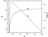 |
Fig. 1. Matching parameter p as a function of the Sérsic index n (solid line) determined by numerically solving Eq. (15) so that the total luminosity of the profile νa(r) in Eq. (13) coincides with L of the true profile in Eq. (1). As explained in Appendix A, p(n) vanishes for n → 1 and then increases for decreasing n < 1 (see Table B.1). The dashed line gives the transition radius (in units of Re) as defined in Eq. (16); for n < 1, st increases for decreasing n, remaining small, however. |
It is also useful to define the transition radius rt as the radius at which νi(rt) = νe(rt); that is, from Eq. (13),
 (16)
(16)
Qualitatively, for distances from the center smaller than st, the profile is dominated by νi(r), while for larger radii, the profile is increasingly better described by νe(r). In Figure 1, the dashed line shows the function st(n). We note the non-monotonicity at low values of n ≲ 2, with a maximum of st ≃ 0.02 reached at n ≃ 1.63, and the following decrease to st(4)≃0.002, st(6)≃0.0002, and so on, with st → 0 for n → 1. These trends can be explained with a careful asymptotic analysis of Eq. (16), which shows that st ∼ π(n − 1)2/[2b(1)] for n → 1+ and st ∼ e1/6/(4πn) for n → ∞. In practice, st is always very small, which is an indication that ν(r) is almost completely dominated by the external asymptotic profile. For the sake of completeness, we note that for n < 1, st instead increases for decreasing n, as illustrated in Figure 1 and proved in Appendix A.
3. Results
We checked the accuracy of νa in Eq. (13) by computing the relative error profile
 (17)
(17)
where ν(r) is the numerically deprojected profile. As ν(r) diverges at the center for n ≥ 1, a poor treatment of the integral in Eq. (4) can easily lead to a significant accuracy loss for small radii, affecting in turn the robustness of the indicator ℰ(r). In order to control the deprojection, we started from Eq. (7) of C91 (which holds for generic n > 0), written in terms of the reduced radius α ≡ bs1/n and where the central divergence of ν(r) for n > 1 is factored out exactly:
![Mathematical equation: $$ \begin{aligned} \nu (r) &= {I_0\over R_{\rm {e}}}{b^n \alpha ^{1-n}\over \pi } \int _1^{\infty } {\mathrm{e}^{-\alpha \, t} dt\over \sqrt{t^{2n} - 1}}\nonumber \\&= {I_0\over R_{\rm {e}}} {b^n \alpha ^{1-n} \mathrm{e}^{-\alpha }\over n \pi } \int _0^\infty {\mathrm{e}^{-\alpha \, [\left(x^2 + 1\right)^{1/(2n)}-1]}\over \left(x^2 + 1\right)^{1 - 1/(2n)}} dx. \end{aligned} $$](/articles/aa/full_html/2025/02/aa52586-24/aa52586-24-eq21.gif) (18)
(18)
In this way, the resulting integral becomes convergent. In the second line, we adopted the substitution  so that the new integrand is free of the singularity, further improving the numerical stability. Motivated by the functional form of Eqs. (10)–(11), we finally factored out the exponential term e−α.
The results are surprisingly good and qualitatively similar for all values of n, with accuracy increasing for increasing n. The profile of ℰ(r) is shown in Figure 2 for the three representative cases of n = 2, 4, and 8; the largest error occurs at small radii. In general, νa(r) tends to overestimate the true ν(r) at small radii before converging to it (by construction) for r → 0. Similarly, at large radii, νa(r) tends to underestimate the true profile before converging to it (by construction) for r → ∞. This behavior is due to the fact that while νa(r) lies below νi(r) and νe(r), the leading terms νi(r) and νe(r) remain above the true ν(r). In the central regions, ν(r) < νa(r) < νi(r), and in the external parts, νa(r) < ν(r) < νe(r). Of course, for r → 0 and r → ∞, the two inequalities become equalities.
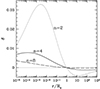 |
Fig. 2. Radial trend of the relative error in Eq. (17) between the asymptotically matched and the numerically deprojected profiles for n = 2, 4, and 8. |
Table 1 reports (with its sign) the maximum relative deviation of ℰ(r) over the whole radial range and the radius smax at which the maximum deviation is reached. As also shown in Figure 2, smax moves toward the center and ℰmax decreases for increasing n. When smax < 10−4 (corresponding to models with n ≳ 4.2), the largest deviation is reached at radii where a continuous stellar density profile lacks astrophysical meaning and in the ℰmax column, we just report the value of  at s = 10−4. In general, this value is the maximum deviation for all s > 10−4 due to the shape of ℰ(r).
Maximum relative errors.
To quantify the deviation of νa(r) from the true profile, we also considered the radial trend of the difference (in magnitudes) between the Sérsic profile in Eq. (1) and the projected profile Ia(R) obtained from νa(r). That is, we considered
 (19)
(19)
Figure 3 shows Δμ(R) for the n = 2, 4, and 8 profiles. The behavior is qualitatively similar for all n > 1. As expected, the errors are extremely small, and they decrease for increasing n, confirming that the accuracy of νa(r) is such that it can certainly be used for all practical purposes. In Columns (4) and (5) of Table 1, we report the maximum magnitude difference and the radius at which it is reached for representative values of n. Again, when the maximum deviation is reached inside s = 10−4, we give the magnitude difference at s = 10−4.
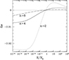 |
Fig. 3. Difference in magnitude associated with the projected profile obtained from the asymptotically matched density νa(r) in Eq. (13) and the true Sérsic profiles with n = 2, 4, and 8. |
Of course, it is particularly important that the errors compare well with those obtained from other high-accuracy fitting methods (e.g., Vitral & Mamon 2020) but are now associated with a mathematically motivated, algebraically simple, and (except for the p value) fully analytical formula. We stress again that this formula is not the result of a fit.
4. Conclusions
The Sérsic law is the standard profile to describe the surface brightness of early-type galaxies and other astrophysical systems. Unfortunately, its deprojection ν(r) cannot be expressed in terms of elementary functions for generic values of the shape parameter n. Even though nowadays a numerical deprojection can be performed very efficiently and with arbitrarily high accuracy thanks to powerful computer algebra systems, in some applications the availability of simple and manageable formulae can be useful. In fact, over the years several analytical approximations of ν(r) have been proposed, and some of these formulae are very accurate, but in general they are based on “ad hoc” fits of the numerical ν(r) deprojection over some radial range and are therefore missing – with some exceptions – the correct asymptotic behavior of ν(r) at small and large radii. They also may require the input of several numerically determined coefficients, which are sometimes given as tables.
In this work, we followed a different approach. We constructed a simple algebraic formula νa(r), which is not more complicated than a rational function, to approximate the true ν(r) for n > 1. The derived formula is not a fitting formula. It contains only two analytical coefficients that depend on n, and it came from requiring νa(r) to be asymptotically exact at small and large radii and to reproduce the monotonic decrease of ν(r) with r when n ≥ 1/2. The two asymptotic regimes are joined with the introduction of a matching parameter p(n) with a value uniquely determined by the request that the total luminosity of νa(r) be the same as that of the original Sérsic profile of same index n, effective radius Re, and central surface brightness I0. A grid of values of p(n) is provided in Table B.1 for 0.55 ≤ n ≤ 11.6; further values of p(n) can be easily computed by interpolation or numerical integration of Eq. (15). It is also possible to produce high-accuracy analytical interpolation formulae for p(n), but we did not pursue this possibility in this paper. We tested νa(r) against the true ν(r), and we found its accuracy impressive at all radii, especially considering its extreme simplicity. The maximum absolute value of the relative difference between ν(r) and νa(r) decreases for increasing n and is of the order of ≃10−3 for n ≳ 4. For example, for the R1/4 law in the range 0.1Re < R < 10Re, relative errors are smaller than 0.002. The accuracy of the formula was also tested by projecting νa(r) and then comparing the surface brightness profile with that of the Sérsic law, expressed in magnitudes. The maximum absolute value of the relative difference is very small, smaller than 0.05 mag in the worst low-n case reported, decreasing to 0.007 mag for the de Vaucouleurs profile and to 0.002 mag or less for larger values of n. Due to its simplicity, high accuracy, and the fact that its properties came from imposing a match with the known properties of the true deprojected Sérsic law, we believe the νa(r) in Eq. (13) is the best (theoretically motivated) compromise currently available between simplicity and accuracy.
Finally, we note that the generalization of the formula to axisymmetric and triaxial ellipsoidal systems is immediate. In fact, in order to describe a Sérsic triaxial system of total luminosity L stratified on
 (20)
(20)
with a ≥ b ≥ c, in the expression for νa(r) in Eq. (13), one substitutes the scaled radius s with m and Re with a and then divides the resulting formula by the product qyqz. In this way, the total luminosity of νa(m) is independent of the flattening. The projection of νa of such a triaxial system at any inclination of the line of sight can be done as described in Chapter 11 in C21. In particular, it turns out that a is the semimajor axis of the effective isophotal ellipse when projecting νa(m) along the intermediate (y) or short (z) axis, and its value coincides with Re of the spherical limit of νa(m). This ellipsoidal generalization of νa(r) could be a useful improvement for the modeling technique based on triaxial Sérsic ellipsoids presented in van de Ven & van der Wel (2021).
Due to a typo, the coefficient 2mbm − 1 at the denominator of Eq. (9) in C91 and of Eq. (13.25) in C21 (for m > 1) should be 2πmb−1. We notice that Eq. (A5) in C91, from which the correct Eq. (10) in this paper and the two mentioned equations in C91 and C21 are derived, is correct. Again, due to a typo in Eq. (13.25) in C21 (for m = 1), the s1/2 at the denominator should be s, as in the correct Eq. (7) in this paper and (A6) in C91.
Volume integration of Eq. (13) in the limit of n → ∞ can be performed noticing that the denominator of νa tends to the constant (1 + πp/2)1/p so that an asymptotic analysis shows that the limit value of p is given by the solution of 1 + πp/2 = 2p, in agreement with the value determined from the numerical integration described in the text.
Acknowledgments
We thank the Referee, Gary Mamon, for a very careful reading of the manuscript, insightful comments and useful suggestions. LDD thanks Arjen van der Wel for useful discussions.
References
- Andredakis, Y. C., Peletier, R. F., & Balcells, M. 1995, MNRAS, 275, 874 [NASA ADS] [CrossRef] [Google Scholar]
- Baes, M., & Ciotti, L. 2019, A&A, 630, A113 [NASA ADS] [CrossRef] [EDP Sciences] [Google Scholar]
- Baes, M., & Gentile, G. 2011, A&A, 525, A136 [NASA ADS] [CrossRef] [EDP Sciences] [Google Scholar]
- Baes, M., & Van Hese, E. 2011, A&A, 534, A69 [NASA ADS] [CrossRef] [EDP Sciences] [Google Scholar]
- Barmby, P., McLaughlin, D. E., Harris, W. E., Harris, G. L. H., & Forbes, D. A. 2007, AJ, 122, 2458 [Google Scholar]
- Battaglia, G., Tolstoy, E., Helmi, A., et al. 2006, A&A, 459, 423 [NASA ADS] [CrossRef] [EDP Sciences] [Google Scholar]
- Bendinelli, O., Ciotti, L., & Parmeggiani, G. 1993, A&A, 279, 668 [NASA ADS] [Google Scholar]
- Binney, J., & Tremaine, S., 2008, Galactic Dynamics 2nd edition (Princeton University Press) [Google Scholar]
- Caon, N., Capaccioli, M., & D’Onofrio, M. 1993, MNRAS, 265, 1013 [NASA ADS] [CrossRef] [Google Scholar]
- Ciotti, L. 1991, A&A, 249, 99 (C91) [NASA ADS] [Google Scholar]
- Ciotti, L. 2021, Introduction to Stellar Dynamics (Cambridge University Press) (C21) [CrossRef] [Google Scholar]
- Ciotti, L., & Bertin, G. 1999, A&A, 352, 447 [NASA ADS] [Google Scholar]
- de Vaucouleurs, G. 1948, Ann. d’Astroph., 11, 247 [Google Scholar]
- Emsellem, E., & van de Ven, G. 2008, ApJ, 674, 653 [CrossRef] [Google Scholar]
- Gerbal, D., Lima, Neto G. B., Márquez I., Verhagen H., 1997, MNRAS, 285, L41 [NASA ADS] [CrossRef] [Google Scholar]
- Gradshteyn, I. S., & Ryzhik, I. M. 2007, Table of Integrals, Series, and Products, 7th edn. (Elsevier) [Google Scholar]
- Graham, A. W., & Driver, S. P. 2005, PASA, 125, 118 [NASA ADS] [CrossRef] [Google Scholar]
- Graham, A. W., & Guzman, R. 2003, AJ, 22, 2936 [NASA ADS] [CrossRef] [Google Scholar]
- Lima, Neto G. B., Gerbal D., & Márquez I., 1999, MNRAS, 309, 481 [NASA ADS] [CrossRef] [Google Scholar]
- Márquez, I., Lima, Neto G. B., Capelato H., Durret F., & Gerbal D., 2000, A&A, 353, 873 [Google Scholar]
- Mazure, A., & Capelato, H. V. 2002, A&A, 383, 384 [NASA ADS] [CrossRef] [EDP Sciences] [Google Scholar]
- Mellier, Y., & Mathez, G. 1987, A&A, 175, 1 [NASA ADS] [Google Scholar]
- Pechetti, R., Seth, A., Neumayer, N., et al. 2020, ApJ, 900, 32 [NASA ADS] [CrossRef] [Google Scholar]
- Poveda, A., Iturriaga, R., & Orozco, I. 1960, BOTT, 2, 3 [NASA ADS] [Google Scholar]
- Prugniel, P., & Simien, F. 1997, A&A, 321, 111 [NASA ADS] [Google Scholar]
- Sérsic, J. L. 1968, Atlas de Galaxias Australes (Cordoba, Argentina: Observatorio Astronomico) [Google Scholar]
- Simonneau, E., & Prada, F. 2004, RMxAA, 40, 69 [NASA ADS] [Google Scholar]
- Terzić, B., & Graham, A. W. 2005, MNRAS, 362, 197 [CrossRef] [Google Scholar]
- Trujillo, I., Asensio, Ramos A., Rubiño-Martín, J. A., et al. 2002, MNRAS, 333, 510 [NASA ADS] [CrossRef] [Google Scholar]
- van de Ven, G., & van der Wel, A. 2021, ApJ, 914, 45 [NASA ADS] [CrossRef] [Google Scholar]
- Vitral, E., & Mamon, G. A. 2020, A&A, 635, A20 [EDP Sciences] [Google Scholar]
- Vitral, E., & Mamon, G. A. 2021, A&A, 646, A63 [NASA ADS] [CrossRef] [EDP Sciences] [Google Scholar]
- Young, P. J. 1976, AJ, 81, 807 [NASA ADS] [CrossRef] [Google Scholar]
Appendix A: The asymptotically matched formula for n ≤ 1
The paper is mainly focused on the case of Sérsic profiles with n > 1. However, it is of interest to illustrate how the proposed approach works for the cases n ≤ 1.
We first show that the point-wise limit of equation (13) for n → 1+ and an arbitrary but fixed p > 0 converges to the profile
 (A.1)
(A.1)
In fact the coefficients c1 and c2 in equation (14) both diverge for n → 1, due to the divergence of the beta function as 2/(n − 1); in particular, the divergence of c2 implies that for arbitrary but fixed p > 0, νa in equation (13) converges everywhere to the profile νe of the n = 1 deprojected density in equation (7). The volume integral of νa(r) in equation (A.1) gives a total luminosity of  . Therefore, for a generic but fixed p > 0, the total luminosity of the pointwise limit of νa in equation (13) for n → 1 does not converge to the total luminosity of the true n = 1 profile (even if it is quite close to it). Of course, this behavior is to be expected, as the limit of νa for n → 1 should be taken not at a fixed p, but along the sequence p(n) defined implicitly by equation (15), so that the conservation of total L is guaranteed. It follows immediately that limn → 1+p(n) = 0, because for any strictly positive limit value p(1) > 0, equation (A.1) would be reobtained, violating the total luminosity conservation. In fact, p(n) is numerically found already below unity for n = 1.05 (see Table B.1), with values monotonically decreasing for decreasing n toward unity (see Table B.1).
Next, we consider the n < 1 profiles. From equations (9) and (11) it follows that for 1/2 < n < 1 again  for s → ∞, and
  for s → 0 so that the arguments used to build equation (13) still apply, and then
![Mathematical equation: $$ \begin{aligned} \nu _{\rm a}(r) = \displaystyle {\nu _{\rm {i}}(r)\over \left\{ 1 +\left[\nu _{\rm {i}}(r)/\nu _{\rm {e}}(r)\right]^p\right\} ^{1/p}} ={L\over R_{\rm {e}}^3}{c_1\,\mathrm{e}^{-b\, s^{1/n}}\over \left[1 + c_2^p\, s^{p-p/(2n)}\right]^{1/p}}, \end{aligned} $$](/articles/aa/full_html/2025/02/aa52586-24/aa52586-24-eq32.gif) (A.2)
(A.2)
where
 (A.3)
(A.3)
For n = 1/2, the deprojected Sérsic profile is Gaussian
 (A.4)
(A.4)
where b = b(1/2) = ln2 and  ; that is, for n = 1/2, the true deprojected profile coincides at all radii with the asymptotic profiles in equations (9) and (11). It follows that
  everywhere, and then equations (A.2) and (15) require that limn → 1/2+p(n) = ∞. This is nicely confirmed by the numerically recovered values of p (see Table B.1).
As for the n > 1, it is natural to define the transition radius rt, where νi(rt) = νe(rt), and from equation (A.2) we obtain the analogous of equation (16)
 (A.5)
(A.5)
Again, a careful asymptotic analysis shows that st ∼ π(n − 1)2/[2b(1)] for n → 1−, while  , in agreement with Figure 1: notice however that for n = 1/2 the concept of transition radius loses its meaning, because
  everywhere.
For the sake of completeness, we also consider the range 0 < n < 1/2, where the situation changes. In fact, now  for s → ∞ and diverges for s → 0, so that equation (A.2) with a positive p would fail to reproduce the correct asymptotic trends of the true profile. However, it is not difficult to show that νa(r) in equation (A.2) with negative values p recovers the asymptotic trends of the true deprojected ν(r).
In analogy with equation (18), we finally give the integral expression of ν(r) to be used for high-accuracy deprojection when n < 1
![Mathematical equation: $$ \begin{aligned} \nu (r) = {I_0\over R_{\rm {e}}} {b^n \mathrm{e}^{-\alpha }\over n\pi } \int _0^\infty { \mathrm{e}^{-[\left(x^2 + \alpha ^{2n}\right)^{1/(2n)}-\alpha ]} \over \left(x^2 + \alpha ^{2n}\right)^{1 - 1/(2n)} } dx, \end{aligned} $$](/articles/aa/full_html/2025/02/aa52586-24/aa52586-24-eq41.gif) (A.6)
(A.6)
obtained with the change of variable x = t/αn in equation (18). Notice that equation (A.6) avoids the problem of equation (18) when used with n < 1, namely the fact that the factor α1 − n therein would vanish for s → 0, and the integral would diverge, as obvious from the fact that ν(0) is finite for n < 1.
Appendix B: Numerically determined values of p(n)
Table B.1 gives the values of the matching parameter p in equation (13) for a grid of values of n. Two decimal digits of p(n) are sufficient to guarantee that the total luminosity of νa(r) is the same as that of the Sersic profile of given I0, Re and n, with relative differences smaller than 10−3 for all values of n reported; with three decimal digits the differences become much smaller than 10−4. For values of n not reported in the Table, p(n) can be easily computed by numerical integration of equation (15), or by numerical interpolation of the values provided.
A grid of values of the matching parameter p(n).
All Tables
All Figures
|
Fig. 1. Matching parameter p as a function of the Sérsic index n (solid line) determined by numerically solving Eq. (15) so that the total luminosity of the profile νa(r) in Eq. (13) coincides with L of the true profile in Eq. (1). As explained in Appendix A, p(n) vanishes for n → 1 and then increases for decreasing n < 1 (see Table B.1). The dashed line gives the transition radius (in units of Re) as defined in Eq. (16); for n < 1, st increases for decreasing n, remaining small, however. |
| In the text | |
|
Fig. 2. Radial trend of the relative error in Eq. (17) between the asymptotically matched and the numerically deprojected profiles for n = 2, 4, and 8. |
| In the text | |
|
Fig. 3. Difference in magnitude associated with the projected profile obtained from the asymptotically matched density νa(r) in Eq. (13) and the true Sérsic profiles with n = 2, 4, and 8. |
| In the text | |
Current usage metrics show cumulative count of Article Views (full-text article views including HTML views, PDF and ePub downloads, according to the available data) and Abstracts Views on Vision4Press platform.
Data correspond to usage on the plateform after 2015. The current usage metrics is available 48-96 hours after online publication and is updated daily on week days.
Initial download of the metrics may take a while.