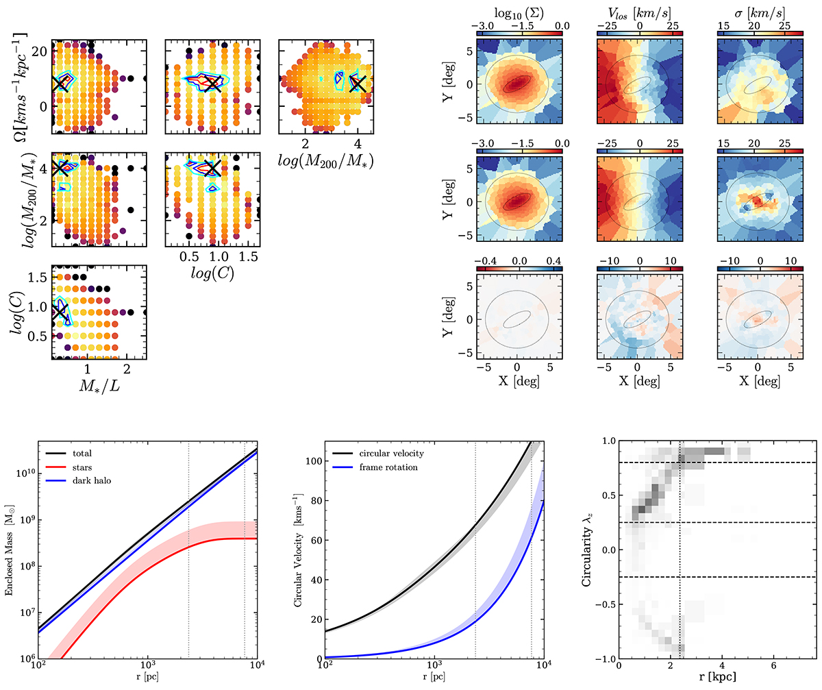
Schwarzschild model results. Top-left panel: Full grid of Schwarzschild models (potential parameters and bar pattern speed) that we computed, colour-coded by χ². The best-fit model is indicated with a cross, and the one-, two-, and three-σ contours are overplotted with red, blue, and cyan, respectively. Top-right panel: Performance of the best Schwarzschild model with Ω = 8 km s⁻¹ kpc⁻¹. Top-row: Model input. This includes surface brightness MGE, LOS velocity, and smoothed LOS velocity dispersion. Middle row: Model output. This contains the same quantities as computed from the weighted orbits superposition. Bottom row: Model residuals. Bottom-left panel: Enclosed cumulative mass profiles of the stellar (M_*/L = 0.3 M_⊙/L_⊙), DM, and total mass distributions according to the best-fit Schwarzschild model. Bottom-middle panel: Circular velocity curve according to the same model together with the frame rotation with Ω = 8 km s⁻¹ kpc⁻¹. The shaded regions in both panels indicate the 1σ confidence intervals. Bottom-right panel: Orbit weights as a function of their circularity and radius for the best-fit model. The vertical line denotes the size of the bar, and the horizontal lines differentiate different types of orbits: λ_z ∼ 0 are radial orbits, λ_z ∼ 1 are highly circular orbits, and λ_z < 0 are retrograde.