| Issue |
A&A
Volume 692, December 2024
|
|
|---|---|---|
| Article Number | A38 | |
| Number of page(s) | 7 | |
| Section | Numerical methods and codes | |
| DOI | https://doi.org/10.1051/0004-6361/202449431 | |
| Published online | 29 November 2024 | |
SiamVIT: A patchwise network for γ-ray point source detection
1
School of Computer Science and Engineering, Xi’an Technological University, Xi’an
710021,
Shaanxi,
China
2
State and Local Joint Laboratory of Advanced Network and Monitoring, Xi’an,
710021,
Shaanxi,
China
★ Corresponding author; This email address is being protected from spambots. You need JavaScript enabled to view it.
Received:
31
January
2024
Accepted:
1
October
2024
Abstract
Aims. Conventional point source detection methods generally work in a pixelwise manner and can hardly exploit the overall semantic information of sources; consequently, these methods usually suffer from low precision. In this work we achieve point source detection in fully patchwise mode by proposing a siamese network called SiamVIT that includes a visual transformer (VIT). SiamVIT can effectively and accurately locate point sources from γ-ray maps with high purity not only in higher flux regions, but also in lower flux regions, which is extremely challenging to achieve with state-of-the-art methods.
Methods. SiamVIT consists of two VIT branches and a matching block. In the feature extraction stage, γ-ray maps are fed into one VIT branch to obtain patch representations with adequate semantic and contextual information, whereas detection templates with location information are fed into the other branch to produce template representations. In the location stage, a patch representation and all template representations are fed into the matching block to determine whether the associated γ-ray map patch contains a point source and where that point source is located, if applicable.
Results. We compare our proposed SiamVIT with the current advanced methods and find that SiamVIT has significantly better purity and completeness and a superior Dice coefficient on the test set. In addition, when point sources overlap, SiamVIT can better distinguish different point sources.
Key words: methods: data analysis / techniques: image processing / gamma rays: general
These authors are co-second authors, having equally contributed to this work without any ranking distinction.
© The Authors 2024
 Open Access article, published by EDP Sciences, under the terms of the Creative Commons Attribution License (https://creativecommons.org/licenses/by/4.0), which permits unrestricted use, distribution, and reproduction in any medium, provided the original work is properly cited.
This article is published in open access under the Subscribe to Open model. This email address is being protected from spambots. You need JavaScript enabled to view it. to support open access publication.
1 Introduction
Point source detection plays a crucial role in astronomical research. By detecting and analyzing point sources, not only are we able to discover new stars and study the internal structure and composition of the Milky Way, but also to delve into the nature and evolution trends of distant galaxies and quasars. Point source detection also provides significant convenience for studying interactions between celestial bodies, such as the gravitational interactions occurring among stars and the impacts of active galactic nuclei. These advancements have driven the development of astronomy, and also broadened our understanding of the universe as a whole. In the γ-ray band, point source detection provides insight into high-energy astrophysical phenomena such as gamma-ray bursts, pulsars, and active galactic nuclei, helping to characterize extreme energy processes in the cosmos.
Since the deployment of the Fermi large area telescope (Fermi-LAT), numerous celestial bodies emitting high-energy γ-ray radiation have been detected. Discovering new point sources from these gamma-ray emissions may contribute significantly to the construction of astronomical source catalogs. Generally, a point source can be assumed to have a typical shape similar to that of a Gaussian distribution. Since a point source is small, potentially dim, and easily disturbed by background clutter, attaining satisfactory detection performance with the Fermi-LAT data is still challenging.
The traditional technical route for point source detection is to artificially design a feature extractor according to several point source priors (e.g., a small area, strong local contrast) and convert the intensity of the view field into a feature saliency map. Then, several rules are used to locate the most salient area in the saliency map as the point source. In recent years, with the development of deep learning techniques, neural networks have gradually replaced artificially designed feature extractors for obtaining target features (Vafaei Sadr et al. 2019, Panes et al. 2021, Stoppa et al. 2022). Owing to the strong representation capabilities of neural networks, the point source detection accuracies of related methods have greatly improved.
However, most traditional and deep learning methods apply pixelwise processing in their key steps. For example, the final detection stage generally checks the saliency map in a pixel-by-pixel manner to determine whether a pixel belongs to the target point source or the background. Pixelwise methods may suffer from low accuracy since they fail to use the overall semantic and contextual information of sources effectively. However, this information is crucial for differentiating a point source from the background and clutter (as shown in Fig. 1).
On the basis of the above considerations, we propose a deep learning method that exploits the semantic and contextual information of a point source (see Fig. 2). First, an input γ-ray map is divided into patches, and the point source may be detected in one of these patches. Second, the γ-ray map patches and a set of trained templates containing location information are both fed into a siamese visual transformer (VIT) to extract features. Finally, the extracted patch features and template features are sent to a feature-matching module to evaluate their matching similarity and to determine whether each patch contains the point source and where the point source is located according to the matching results. For simplicity, the proposed deep neural network is called a SiamVIT. The proposed SiamVIT method employs the overall semantic information of the point sources in both the feature extraction and matching stages. In addition, with the aid of the VIT structure, the contextual semantic information of the point source is fully utilized. The experimental results demonstrate that the purity, completeness, and Dice coefficient achieved by the SiamVIT method on the employed test set are significantly better than those of other existing methods.
There are two main aims for this work. First, our aim was to detect point sources as a whole (DSW) to avoid traditional pixellevel processing and to fully utilize the contextual semantics of point sources by proposing the SiamVIT method, which regards γ-ray map patches as unified entities.
Second, comprehensive comparative experiments and ablation studies were conducted to demonstrate the superiority of the proposed SiamVIT method. Specifically, SiamVIT offers obvious advantages over other approaches in terms of both utilized metrics.
The paper is organized as follows. In Section 2, we briefly review the related work. In Section 3, we introduce the architecture of our SiamVIT in detail. The experimental results are described in Section 4. Section 5 provides the conclusion.
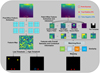 |
Fig. 1 Traditional pixelwise method (left panel) and our patchwise method (right panel). In the left panel, the point source and the bright region in the background have similar intensities; thus, they have similar saliency levels in the saliency map obtained via a typical existing method. They are similarly judged as point sources or backgrounds in the subsequent pixel-by-pixel thresholding-based segmentation step, resulting in an FP (where the bright region is judged as a point source) or an FN (where the point source is judged as background). The typical point source intensity distribution is an approximate Gaussian distribution. Additionally, the point source is isolated, as it is very different from a bright region that connects with other bright regions. By utilizing this overall information and the contextual semantics of the point source, our proposed method accurately matches and localizes the point source while rejecting the bright region via templates (right panel). |
2 Related works
2.1 VITs
Initially, transformers (Vaswani et al. 2017) were applied to natural language processing tasks by measuring the relationships between input words. Following the transformer mechanism, the original VIT (Dosovitskiy et al. 2021) was used to compute the relationships among fixed-size image patches by linearly embedding each of them and then feeding the obtained sequence of vectors to a standard transformer encoder. In this way, patch representations containing contextual information were easily extracted. VITs have been proven to be powerful methods in multiple computer vision tasks, including image classification, semantic segmentation, and target detection.
2.2 Point source detection
Traditional methods (Masias et al. 2012) use discontinuity priors between point sources and backgrounds. Filtering methods (Yang et al. 2008; Freeman et al. 2002, and Lang et al. 2010) employ a sliding window approach, in which a specific statistical metric (such as the median or mean) is computed over all image pixels within the window. By utilizing the calculated values, this method replaces all the pixels in the window, effectively filtering noise and smoothing the image. Background suppression methods (Perret et al. 2009; Haupt et al. 2009) first adopt smoothness filters to filter out the point sources in the input image to obtain a pure background. The potential targets can be detected by subtracting the estimated background from the original image. Multiscale methods (Starck & Murtagh 2007; Starck et al. 2009; Gonzalez-Nuevo et al. 2006) employ appropriate techniques to map the intricate hierarchical structure within astronomical data to a multiscale space. These methods decompose the data into components at different scales and subsequently apply fundamental detection algorithms to identify point sources at these scales.
Recently, deep learning techniques have been applied to point source detection tasks. Deep learning methods typically use the concept of image segmentation, designing neural network models manually or through transfer learning to convert astronomical images into binary masked images for point source detection. A convolutional neural network (CNN) was used to increase the signal-to-noise ratio (S/N) of an original map, and dynamic blob detection was used to detect point sources (Vafaei Sadr et al. 2019). Panes et al. (2021) and Stoppa et al. (2022) viewed point source detection as an image segmentation task. First, they used a U-Net image segmentation network (Ronneberger et al. 2015) to segment the target point source from the background image, obtaining its feature saliency map. Then, they used the thresholding method to highlight the point source on the feature saliency map.
The technical steps of the above method can be summarized as follows. First, a feature extractor is artificially designed according to the point source priors or learned from a large quantity of data. This extractor is subsequently used to convert the input image into a feature saliency map. Finally, a rule, for example thresholding, is employed to locate the most salient region as the point source. However, most of the above methods use a pixel-by-pixel approach for feature extraction or point source segmentation, which is not conducive to making full use of the overall semantic and contextual information of the target point source. Consequently, our work focuses on solving this problem by treating image patches as entities, and the details of the proposed method are illustrated below.
3 Proposed methods
3.1 Overview of the method
A γ-ray map with a size of Wi × Hi is equally divided into M × N patches with sizes of W × H. Notably, W = Wi/M and H = Hi/N. In practice, W and H are slightly larger than the typical size of a point source; hence, a patch can contain a complete point source. We pregenerate W × H representative templates of different point source locations. When SiamVIT is working, the patch on which the center of the point source falls is responsible for locating the point source. The workflow is as follows (as shown in Fig. 2). First, the γ-ray map patches and the template are input into two VIT branches to obtain their features. Then, the features of each template are input into the matching block individually to calculate the matching degree with each γ-ray map patch feature. If a template and a patch obtain a high matching degree, the patch may contain a point source, and the location of the point source in the patch is the same as the location of the point source in the template. Otherwise, the patch is judged to contain no point sources. The key elements of our approach are described in detail in the subsequent sections.
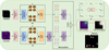 |
Fig. 2 SiamVIT. The upper and lower branches are both VIT structures. The upper branch processes templates containing location information. Its number of feature embeddings is equal to the number of templates. The lower branch processes γ-ray map information, and its number of feature embeddings equals the number of patches in the γ-ray map. The inputs of the matching block are the feature embeddings of the template and the γ-ray map, and the output is a matrix. A patch corresponding to high values in the matrix may contain a point source, and the position of the point source is the same as the position of the point source in the template corresponding to the high values. |
3.2 Templates
We construct a set of learnable templates that mimic the intensity distributions of typical point sources. The template size is the same as the γ-ray map patch size: W × H. We construct W × H templates, each with the point source center located at one of the W × H locations. The initial intensity values of the templates are generated in this way to facilitate convergence during training. As shown in Fig. 3, first, we generate a Gaussian matrix with a size of (2W − 1) × (2H − 1) centered at (W, H) to simulate the intensity distribution of a typical point source. Then, we use a window with a size of W × H to slide from the lower right of the Gaussian matrix to the upper left with a step size of 1, and the submatrix covered by each window is saved as a template. In this way, W × H templates are obtained. These templates are subject to the same Gaussian distribution, but their centers are located at different locations from the upper left to the lower right. Notably, the use of a Gaussian distribution to approximate the point source distribution is reasonable, even though more precise models such as a combination of King functions are available (Read et al. 2011, Malyshev & Hogg 2011). SiamVIT relies primarily on the characteristics of the point source core region. It identifies the presence of a point source and estimates its exact location by matching this core region to a template. Focusing on the core features for detection and localization is particularly advantageous in crowded areas as it helps reduce interference from nearby point sources. Given that the core region of point sources generally follows a Gaussian distribution (Masias et al. 2012; Abdollahi et al. 2020), this approximation provides adequate accuracy for our work. Additionally, we set the templates to be learnable, so even though the initial distributions of the templates are Gaussian, they can be dynamically adjusted during training to more accurately capture the true distribution characteristics of the point sources.
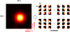 |
Fig. 3 Initial template generation process. First, we generate a Gaussian matrix with a size of (2W − 1) × (2H − 1) centered at (W, H) to simulate the intensity distribution of a typical point source. Then, we use a window with a size of W × H to slide from the lower right of the Gaussian matrix to the upper left by utilizing a step size of 1. Each submatrix covered by the window is saved as a template. |
3.3 SiamVIT branches
Two siamese VIT branches are used to extract features from the γ-ray maps and templates. When extracting γ-ray map features, we split the γ-ray map into fixed-size patches, linearly embed them, add position embeddings, and feed the resulting patch embedding sequence to the γ-ray map branch. The number of embedding blocks equals the number of patches in the γ-ray map. When passing through the transformer, each embedded patch, as a whole semantic unit, always interacts with the other embedded patches.
The final representation of a patch contains the overall and contextual point source semantics, which facilitates the subsequent determination of the point source location. The template branch is a transformer encoder similar to the γ-ray map branch, which extracts only the features of a single template. We directly linearly embed a template, feed the single embedding to the template branch, and finally obtain a template representation.
The VIT branches should have the following functions after training: if a patch contains a point source and the point source center is the same as the point source center of a certain template, then the point source representation obtained by the γ-ray map branch should substantially match the template representation obtained by the template branch; conversely, if the patch and a template have different point source locations, then their representations should not match. Additionally, the representation of a background patch that does not contain any point source pixels should not match the representation of either template.
3.4 Feature matching
The feature-matching block inputs the learned patch and template representations. It matches a γ-ray map patch and a template on the basis of their similarity in the embedding space.
Formally, we compute the similarity matrix [Aij] (i, j = 1, 2, ..., W × H) between the i-th template representation ti and the j-th patch representation pj via the Softmax operation computed over the template representations and patch representations as
![Mathematical equation: $\[A_{i j}=\frac{exp(w_{q} t_{i} \cdot w_{k} p_{j})}{\sum_{m=1}^{M \times N} \sum_{n=1}^{M \times N} w_{q} t_{m} \cdot w_{k} p_{n}}\]$](/articles/aa/full_html/2024/12/aa49431-24/aa49431-24-eq1.png) (1)
(1)
where wq and wk are the weights of the learned linear projections for the template and patch representations, respectively.
If the γ-ray map patch and template representations are very similar, the patch may contain a point source, the location of which is the same as the point source location in the template. If a patch representation is not similar to any template representation, the patch may contain no point sources. If a patch contains multiple point sources, it will show a high similarity with multiple templates. The results will highlight several high similarity scores, each indicating the location of a point source detected by the model within the patch.
The matching block locates point sources on the basis of the patchwise representations. It makes full use of the overall semantic point source information, which is conducive to achieving improved location accuracy. Figure 4 shows the result obtained via our patchwise method and the result obtained via an ordinary pixelwise method (Panes et al. 2021). Our method locates the point sources more accurately. Additionally, a high score directly indicates a point source center; in contrast, the ordinary method needs to perform pixelwise clustering on the saliency map to finally obtain the point source location. This results in a relatively high FN rate.
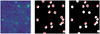 |
Fig. 4 Detection results of the SiamVIT (middle) and UNEK (right) methods. A red cross represents the center of a point source, and the associated white part represents the area where the point source is located; these areas are solid circles with radii of 2.5 pixels. Compared with UNEK, our method locates point sources more accurately. |
3.5 Loss function
When training SiamVIT, we send the γ-ray map patches and templates to the network and obtain a similarity matrix indicating the point source locations. We adopt the MSE loss function
![Mathematical equation: $\[L=\sum_{i=1}^{W \times H} \sum_{j=1}^{M \times N}\left(A_{i j}-Y_{i j}\right)^{2}\]$](/articles/aa/full_html/2024/12/aa49431-24/aa49431-24-eq2.png) (2)
(2)
where Aij is the similarity defined by Eq. (1) and is labeled Yij = 1 if the j-th patch contains a point source for which the location is the same as the point source location of the j-th template; otherwise, Yij = 0.
4 Experiment
4.1 Evaluation metrics
We utilized the purity and completeness metrics (Vafaei Sadr et al. 2019), which can also be considered precision and recall indicators, respectively, in the object detection tasks to evaluate our model. Purity is defined as
![Mathematical equation: $\[Purity =\frac{T P}{T P+F P}\]$](/articles/aa/full_html/2024/12/aa49431-24/aa49431-24-eq3.png) (3)
(3)
Here TP represents the number of correctly identified positive point sources, and FP represents the number of point sources mistakenly identified by the algorithm as real point sources. Completeness is defined as
![Mathematical equation: $\[Completeness =\frac{T P}{T P+F N}\]$](/articles/aa/full_html/2024/12/aa49431-24/aa49431-24-eq4.png) (4)
(4)
where FN represents the number of true point sources that the algorithm has not found.
Purity is the likelihood of correctly identifying true point sources among all the predicted positives. However, predicting only a few sources and ignoring the majority of them can yield high accuracy while increasing FN. Completeness indicates the probability of correctly predicting TP among the actual positives. In dense point source γ-ray maps, predicting all backgrounds as positive can still result in high completeness.
To avoid the problems that may arise from simply using the purity and completeness metrics mentioned above, we introduced the Dice coefficient, which is defined as
![Mathematical equation: $\[Dice =\frac{2 * T P}{2 * T P+F P+F N}\]$](/articles/aa/full_html/2024/12/aa49431-24/aa49431-24-eq5.png) (5)
(5)
The Dice coefficient is a set similarity measure that is commonly used to calculate the similarity between two samples; the value ranges from [0, 1]. The smaller the similarity is between the output and label, the closer the Dice coefficient is to 0; otherwise, the Dice coefficient is closer to 1.
4.2 Implementation details
We trained and tested our proposed SiamVIT model on a public dataset (DarkMachines community 2021) derived from simulations of γ-ray sky data, with the aim of reproducing the full-sky data obtained by the Fermi-LAT telescope over 9.5 years of data acquisition. Poisson noise was added a posteriori to each map in the dataset to account for the Poisson statistics of the real data (for more details, see Panes et al. 2021). The dataset contains approximately 100 000 medium patches (covering almost 250 instances of the full sky) for training and 16 800 medium patches for testing. Each patch is 64 × 64 pixels in size, covering approximately 10° × 10° of the sky, and is divided into five energy bins (0.5–1, 1–2, 2–7, 7–20, and >20 GeV). The patches in these energy bins can be sent to our SiamVIT together for training. This dataset draws solid disk masks with radii of 2.5 pixels to distinguish the point source areas. We used the center points of these solid disks as the locations of the point sources when training the model.
When training the network, we scaled each γ-ray map to 64 × 64 and then divided the maps into equal-sized patches. In general, for a γ-ray map with a size of 64 × 64, the point source area is less than 5 × 5 pixels. We set the patch size to 8 × 8 to ensure that one patch could contain a complete point source. In this way, a γ-ray map was divided into 8 × 8 patches. Thus, in our experiments, M, N, W, and H were set to 8.
In practice, the actual size and resolution of γ-ray maps may differ from those of the simulated data we used. If the γ-ray map is larger than the size specified in our method, we recommend cropping it into smaller subimages that match our defined dimensions. Conversely, if the γ-ray map is smaller than our specified size, it can be tiled to match the required dimensions. Additionally, the hyperparameters of SiamVIT, such as the number of tokens related to the image size, can be adjusted and the network can be retrained to accommodate images of different sizes. For example, for a 128 × 128 γ-ray map that may contain 256 8 × 8 patches, the number of tokens can be set to 256. In γ-ray maps with higher resolutions, point sources typically occupy more pixels. To ensure the complete capture of the point source characteristics, increasing the patch size to allow it to encompass more point source information is advisable. The network should then be retrained following the technical approach we have outlined.
We utilized a curriculum learning approach to train the network, which was conducted in two phases. In the first phase, the network was trained on the Asimov dataset to obtain the initial weights. In the second phase, Poisson noise was introduced into the Asimov dataset, and the weights derived from the first phase were used as pretrained weights. The network was then further trained on the noise-augmented dataset, leading to the final results. The application of curriculum learning can significantly enhance the convergence rate of a neural network.
All the training steps were performed on NVIDIA TITAN RTX GPUs. We implemented all our models via an optimized PyTorch deep learning framework in NVIDIA GPU-accelerated containers. We processed the data with a batch size of 64 and trained both networks from scratch. For optimization, we used adaptive moment estimation (Adam) (Kingma & Ba 2015) as the solver, with b1 and b2 set to 0.9 and 0.999, respectively. The learning rates were set to 0.00001 in all training phases. We tracked the validation errors across the various iterations, and at the end of the training process we used the weights that yielded the smallest validation errors.
Results obtained on test_F0_B1 and our test set.
4.3 Results
4.3.1 Comparison with state-of-the-art methods
We compared our proposed SiamVIT method with the UNEK method (Panes et al. 2021) on a public dataset (DarkMachines community 2021). The test dataset includes public test data (F0B1) and our own stochastically chosen test data. The F0-B1 dataset consists of 768 γ-ray maps containing approximately 10 314 point sources, and our test set comprises 16 800 γ-ray maps with 231 021 point sources. The detection results are presented in Table 1. Observations reveal that SiamVIT detects more TP samples and fewer FN and FP samples than does the UNEK method on both datasets. Our model achieved high purity and completeness values of 0.94 and 0.76, respectively, with a Dice coefficient of 0.84, demonstrating outstanding performance. Figure 4 shows that our model effectively detects multiple point sources in overlapping scenarios, whereas UNEK predicts multiple overlapping point sources as a single point source.
4.3.2 Influence of photon flux
The photon flux refers to the flow of photons per unit area, and is typically used to describe the intensity of a radiation field. In point source detection tasks, the photon flux directly affects the brightness and observability of the target. A higher photon flux may make the target point source brighter, thereby increasing the saliency of the point source in the γ-ray map, whereas a lower photon flux may make it difficult for the point source to stand out significantly from background noise, resulting in a higher FP rate. By analyzing the performance of the SiamVIT algorithm under different photon flux conditions, we observe that the algorithm exhibits excellent performance under high-throughput point source conditions, while also achieving effective point source detection under low-flux conditions. This finding indicates that SiamVIT achieves superior point source detection performance compared to that of UNEK under different photon flux conditions, providing a more comprehensive solution for practical applications.
In Figs. 5, 6, and 7, we illustrate the performance achieved by SiamVIT and UNEK on the test dataset (F0-B1) and our dataset across all latitudes (b > 0°), as well as specifically at high latitudes (b > 20°) and low latitudes (b < 20°). We present the purity and completeness metrics as functions of the source photon flux S1 (>1 GeV).
Under the condition of b>0°, when S 1 reaches 2.01e-10 and 2.09e-10, SiamVIT demonstrates a completeness score of approximately 0.90 on the F0-B1 and the OURS test sets, respectively. In contrast, UNEK requires S1 values of 4.77e-10 and 6.09e-10, respectively, to achieve a similar completeness score on these two test sets. Under the condition of b < 20°, when S1 reaches 2.21e-10 and 2.34e-10, SiamVIT also achieves a completeness score of approximately 0.90 on the F0-B1 and OURS test sets, respectively. UNEK, however, requires S1 values of 7.85e-10 and 9.91e-10, respectively, to reach this level of performance. Under the condition of b > 20°, when S1 reaches 1.07e-10 and 1.71e-10, SiamVIT again shows a completeness score of approximately 0.90 on both test sets. In comparison, UNEK requires S1 values of 2.82e-10 and 2.82e-10, respectively, to achieve a similar completeness score. In addition, SiamVIT achieves a purity score exceeding 0.90 in the low-photon-flux region under all conditions. This observation highlights the superior performance of SiamVIT in terms of completeness in the lower photon flux region, with a high level of purity. In conclusion, the completeness detection level shows a significant improvement under high-purity conditions, with this effect being particularly pronounced in regions with a low photon flux. Notably, while SiamVIT exhibits stable purity performance for sources in both high- and low-flux regions, the purity metric becomes more sensitive to minor fluctuations in TP and FP in the low-flux region due to the limited number of detected sources. This sensitivity can result in notable changes in purity, even with slight variations in the number of detected sources. This is precisely why we observe a significant fluctuation in the purity value in the low-flux region, as seen in Figs. 5–7.
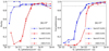 |
Fig. 5 Purity (left) and completeness (right) as functions of the photon flux above 1 GeV, S 1, with a focus on all latitudes. Notably, for some methods in the low-light-flux area, neither true positive nor false positive data can be predicted, making calculation of the purity impossible and therefore preventing it from being plotted on the graph. The same applies to the figures below. |
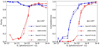 |
Fig. 6 Purity (left) and completeness (right) as functions of the photon flux above 1 GeV, S 1, with a focus on low latitudes. |
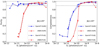 |
Fig. 7 Purity (left) and completeness (right) as functions of the photon flux above 1 GeV, S 1, with a focus on high latitudes. |
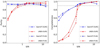 |
Fig. 8 Purity (left) and completeness (right) as functions of the signal-to-noise ratio (S/N). |
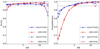 |
Fig. 9 Purity (left) and completeness (right) as functions of the signal-to-background ratio (S/B). |
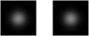 |
Fig. 10 Typical template visualization results. The left panel shows the initialized template; the right panel shows the trained template. |
4.3.3 Influences of the S/N and S/B
In the realm of astronomy, the signal-to-noise ratio (S/N) and signal-to-background ratio (S/B) serve as pivotal metrics for point source detection. The S/N quantifies the signal strength relative to the background noise, whereas the S/B delineates the contrast between the signal and the background. A heightened S/N implies a more salient and easily detectable signal, whereas a diminished S/N suggests susceptibility to noise interference, posing challenges in terms of obtaining accurate detection results. Similarly, an increased S/B underscores a more pronounced distinction between the target celestial body and its surrounding milieu, whereas a lower S/B complicates the process of differentiating the target from the background. In Figs. 8 and 9, our depictions of the intricate relationships among the S/N, S/B, purity, and integrity values produced by the SiamVIT and UNEK methods on the two datasets reveal that the SiamVIT method sustains robust purity and integrity even under low S/N and S/B conditions. When the S/N reaches 1.48 and the S/B reaches 0.742, SiamVIT achieves a completeness score of approximately 0.90 on both the F0-B1 and OURS test sets. In contrast, UNEK requires an S/N of 3.19 and an S/B of 1.05 to achieve a similar completeness score on the F0-B1 test set and an S/N of 2.28 and an S/B of 1.03 to reach comparable performance on the OURS test set. This result demonstrates that, compared with UNEK, SiamVIT exhibits greater noise resilience and superior efficacy in extracting signals from complex astronomical images.
Results obtained before and after performing template training.
Results obtained with different numbers of VIT heads.
4.3.4 Influence of the model structure
We compare the performances of our proposed model when the initialized template and the trained template are used. Table 2 shows the comparison results. Figure 10 shows the visualization results produced for the templates before and after training. The templates observed before and after training are similar, and the model trained with the trained template is not much better than that trained with the initialized template. This shows that it is reasonable to initialize the template as a Gaussian distribution. With limited computing power, the initialized template can be directly used instead of training the template.
We also test variants of the proposed SiamVIT with 1, 2, 4, 8, and 16 heads; the results are shown in Table 3. As the number of heads increases, the accuracy of SiamVIT gradually improves. This proves that increasing the number of heads increases the complexity and representation capabilities of the network, thereby improving its performance. Notably, increasing the number of heads significantly increases the memory consumption of the proposed approach, especially during the training phase. Therefore, we suggest selecting an appropriate number of heads according to the memory conditions encountered in practical applications.
5 Conclusions
In this work, we proposed a DSW rule and accordingly designed a neural network, namely a SiamVIT, for point source detection. The network functions entirely at the patch level and can fully exploit the overall and contextual semantics of point sources. This approach is significantly different from ordinary methods that operate at the pixel level. Comparative experiments show that the proposed method can accurately locate point sources and that it significantly outperforms the existing methods in terms of several indicators.
References
- Abdollahi, S., Acero, F., Ackermann, M., et al. 2020, ApJS, 247, 33 [Google Scholar]
- DarkMachines community 2021, https://doi.org/10.5281/zenodo.4587205 [Google Scholar]
- Dosovitskiy, A., Beyer, L., Kolesnikov, A., et al. 2021, in 9th International Conference on Learning Representations, ICLR 2021, Virtual Event, Austria, May 3–7, 2021 (OpenReview.net) [Google Scholar]
- Freeman, P. E., Kashyap, V., Rosner, R., & Lamb, D. Q. 2002, ApJS, 138, 185 [Google Scholar]
- Gonzalez-Nuevo, J., Argüeso, F., López-Caniego, M., et al. 2006, MNRAS, 369, 1603 [NASA ADS] [CrossRef] [Google Scholar]
- Haupt, J., Castro, R., & Nowak, R. 2009, in Artificial Intelligence and Statistics, PMLR, 216 [Google Scholar]
- Kingma, D. P. & Ba, J. 2015, in 3rd International Conference on Learning Representations, ICLR 2015, San Diego, CA, USA, May 7–9, 2015, Conference Track Proceedings, eds. Y. Bengio, & Y. LeCun [Google Scholar]
- Lang, D., Hogg, D. W., Mierle, K., Blanton, M., & Roweis, S. 2010, AJ, 139, 1782 [Google Scholar]
- Malyshev, D., & Hogg, D. W. 2011, ApJ, 738, 181 [NASA ADS] [CrossRef] [Google Scholar]
- Masias, M., Freixenet, J., Lladó, X., & Peracaula, M. 2012, MNRAS, 422, 1674 [NASA ADS] [CrossRef] [Google Scholar]
- Panes, B., Eckner, C., Hendriks, L., et al. 2021, A&A, 656, A62 [NASA ADS] [CrossRef] [EDP Sciences] [Google Scholar]
- Perret, B., Lefèvre, S., & Collet, C. 2009, Pattern Recogn., 42, 2470 [NASA ADS] [CrossRef] [Google Scholar]
- Read, A., Rosen, S., Saxton, R., & Ramirez, J. 2011, A&A, 534, A34 [NASA ADS] [CrossRef] [EDP Sciences] [Google Scholar]
- Ronneberger, O., Fischer, P., & Brox, T. 2015, in Medical Image Computing and Computer-Assisted Intervention-MICCAI 2015: 18th International Conference, Munich, Germany, October 5–9, 2015, Proceedings, Part III 18 (Springer), 234 [Google Scholar]
- Starck, J.-L., & Murtagh, F. 2007, Astron. Astrophys. Libr. [Google Scholar]
- Starck, J.-L., Fadili, J. M., Digel, S., Zhang, B., & Chiang, J. 2009, A&A, 504, 641 [NASA ADS] [CrossRef] [EDP Sciences] [Google Scholar]
- Stoppa, F., Vreeswijk, P., Bloemen, S., et al. 2022, A&A, 662, A109 [NASA ADS] [CrossRef] [EDP Sciences] [Google Scholar]
- Vafaei Sadr, A., Vos, E. E., Bassett, B. A., et al. 2019, MNRAS, 484, 2793 [CrossRef] [Google Scholar]
- Vaswani, A., Shazeer, N., Parmar, N., et al. 2017, Adv. Neural Inform. Process. Syst., 30 [Google Scholar]
- Yang, Y., Li, N., & Zhang, Y. 2008, in 2008 IEEE International Conference on Systems, Man and Cybernetics, IEEE, 650 [CrossRef] [Google Scholar]
All Tables
All Figures
|
Fig. 1 Traditional pixelwise method (left panel) and our patchwise method (right panel). In the left panel, the point source and the bright region in the background have similar intensities; thus, they have similar saliency levels in the saliency map obtained via a typical existing method. They are similarly judged as point sources or backgrounds in the subsequent pixel-by-pixel thresholding-based segmentation step, resulting in an FP (where the bright region is judged as a point source) or an FN (where the point source is judged as background). The typical point source intensity distribution is an approximate Gaussian distribution. Additionally, the point source is isolated, as it is very different from a bright region that connects with other bright regions. By utilizing this overall information and the contextual semantics of the point source, our proposed method accurately matches and localizes the point source while rejecting the bright region via templates (right panel). |
| In the text | |
|
Fig. 2 SiamVIT. The upper and lower branches are both VIT structures. The upper branch processes templates containing location information. Its number of feature embeddings is equal to the number of templates. The lower branch processes γ-ray map information, and its number of feature embeddings equals the number of patches in the γ-ray map. The inputs of the matching block are the feature embeddings of the template and the γ-ray map, and the output is a matrix. A patch corresponding to high values in the matrix may contain a point source, and the position of the point source is the same as the position of the point source in the template corresponding to the high values. |
| In the text | |
|
Fig. 3 Initial template generation process. First, we generate a Gaussian matrix with a size of (2W − 1) × (2H − 1) centered at (W, H) to simulate the intensity distribution of a typical point source. Then, we use a window with a size of W × H to slide from the lower right of the Gaussian matrix to the upper left by utilizing a step size of 1. Each submatrix covered by the window is saved as a template. |
| In the text | |
|
Fig. 4 Detection results of the SiamVIT (middle) and UNEK (right) methods. A red cross represents the center of a point source, and the associated white part represents the area where the point source is located; these areas are solid circles with radii of 2.5 pixels. Compared with UNEK, our method locates point sources more accurately. |
| In the text | |
|
Fig. 5 Purity (left) and completeness (right) as functions of the photon flux above 1 GeV, S 1, with a focus on all latitudes. Notably, for some methods in the low-light-flux area, neither true positive nor false positive data can be predicted, making calculation of the purity impossible and therefore preventing it from being plotted on the graph. The same applies to the figures below. |
| In the text | |
|
Fig. 6 Purity (left) and completeness (right) as functions of the photon flux above 1 GeV, S 1, with a focus on low latitudes. |
| In the text | |
|
Fig. 7 Purity (left) and completeness (right) as functions of the photon flux above 1 GeV, S 1, with a focus on high latitudes. |
| In the text | |
|
Fig. 8 Purity (left) and completeness (right) as functions of the signal-to-noise ratio (S/N). |
| In the text | |
|
Fig. 9 Purity (left) and completeness (right) as functions of the signal-to-background ratio (S/B). |
| In the text | |
|
Fig. 10 Typical template visualization results. The left panel shows the initialized template; the right panel shows the trained template. |
| In the text | |
Current usage metrics show cumulative count of Article Views (full-text article views including HTML views, PDF and ePub downloads, according to the available data) and Abstracts Views on Vision4Press platform.
Data correspond to usage on the plateform after 2015. The current usage metrics is available 48-96 hours after online publication and is updated daily on week days.
Initial download of the metrics may take a while.