| Issue |
A&A
Volume 691, November 2024
|
|
|---|---|---|
| Article Number | L9 | |
| Number of page(s) | 6 | |
| Section | Letters to the Editor | |
| DOI | https://doi.org/10.1051/0004-6361/202451911 | |
| Published online | 06 November 2024 | |
Letter to the Editor
Blazar S 0528+134 is possibly the most powerful emitter in the Universe, including in the range of gravitational waves
1
Radio Astronomy and Geodynamics Department of Crimean Astrophysical Observatory RAS, Katsively RT-22, Crimea
2
Astro Space Center, Lebedev Physical Institute, Russian Academy of Sciences, Profsoyuznaya ul. 84/32, Moscow 117997, Russia
⋆ Corresponding author; This email address is being protected from spambots. You need JavaScript enabled to view it.
Received:
18
August
2024
Accepted:
23
October
2024
Abstract
Aims. A new method of determining the parameters of close binary systems of supermassive black holes (SMBHs) and the level of gravitational waves (GWs) on the Earth’s surface are proposed.
Methods. Data are presented from long-term monitoring of possibly the most powerful emitter in the Universe, S 0528+134, at five frequencies in the radio range from 4.8 GHz to 37 GHz, obtained by the RT-22 radio telescope of the Radio Astronomy Laboratory CrAO in Simeiz, the RT-26 radio telescope at Michigan Observatory, and the 40 m radio telescope of the Owens Valley Radio Observatory.
Results. The dynamics of powerful flares that have occurred in the object since its discovery in a sky survey in 1970 were considered. The main physical characteristics of binary SMBHs located in the central regions of the system were obtained. These data were used to find the masses of the SMBH companions, the parameters of their orbits, the energy reserve of the system, and the lifetime of the object before the SMBHs’ merger. The level of GWs on the Earth’s surface was determined and the possibility of their detection by International Pulsar Timing Array (IPTA) GW detectors was considered.
Key words: gravitational waves / galaxies: active / BL Lacertae objects: individual: 0528+134 / radio continuum: galaxies
© The Authors 2024
 Open Access article, published by EDP Sciences, under the terms of the Creative Commons Attribution License (https://creativecommons.org/licenses/by/4.0), which permits unrestricted use, distribution, and reproduction in any medium, provided the original work is properly cited.
This article is published in open access under the Subscribe to Open model. This email address is being protected from spambots. You need JavaScript enabled to view it. to support open access publication.
1. Introduction
The era of discovery and study of active galactic nuclei (AGNs) is associated with surveys of decimetre and centimetre waves, beginning in the mid-1960s (Kraus 1966; de Jong 1967; Bolton et al. 1964). An important moment of this time was the discovery of the phenomenon of variable radio sources (Sholomitsky 1965; Dent 1965a,b; Dent & Haddock 1965). The basic catalogues were 3C (Third Cambridge) and 4C, in which many bright radio galaxies and quasi-stellar radio sources (quasars) were discovered (Edge et al. 1959; Scott & Ryle 1961; Bennett & Simth 1962).
The year 1960 was marked by the discovery of a star-like radio source, 3C 48, which has broad emission lines shifted to the red side of the spectrum. It became clear that this was a very distant extragalactic object (Greenstein & Matthews 1963). The extragalactic nature of such objects was finally established in 1963, when Maarten Schmidt determined that the radio source 3C 273 had a redshift of 0.158 and was a quasar (Schmidt 1963). Radio surveys in the 1960s discovered a diverse population of radio galaxies and compact quasars with flat spectra, leading to their classification according to spectral and morphological characteristics (Goss et al. 2023).
As soon as it became clear that variable radio sources have a significant proportion of short-wave radiation, a fast search survey of half of the northern sky was carried out in the USSR in 1969 at a frequency of 8.7 GHz (λ = 3.5 cm) (Larionov et al. 1970, 1971). The survey was conducted on the RT-22 radio telescope of the Crimean Astrophysical Observatory in Simeiz, and was therefore accompanied by the letter ‘S’. Among the newly discovered radio sources, the strongest was S 0528+134, which received the personal name ‘Nimfa’, as, for example, ‘Virgo A’. The presence of this radio source was later confirmed by sky surveys in Ohio and Parkes (Ehman et al. 1974; Wall et al. 1976). An optical identification was made of S 0528+134. It turned out to be a weak point object at 21.5m (Wall & Peacock 1985). Spectroscopy of this source made it possible to determine its redshift, which was z ≈ 2.07 (Hunter et al. 1993).
At the time of discovery of S 0528+134 in radio bands, its flux density was 4.75 Jy at 8.7 GHz. The source was in an active state near its emission maximum. The most intensive study of this source in 1992–1994, when a strong flare occurred in this object and it became one of the most powerful emitters in the Universe. Like other members of this class of sources, S 0528+134 exhibits radio flux variations across multiple timescales ranging from weeks to many years (Aller et al. 1985).
As was already noted, in the optical range the source is weak, including due to strong absorption in the Galaxy. The low galactic latitude of S 0528+134 (bII ≈ −11°) and the dust and molecular clouds in the direction to the object lead to the absorption radiation of S 0528+134 from the optical to X-ray wavelength ranges spanning at least five magnitudes (Zhang et al. 1994). In the range (30 meV–30 GeV) of the CGRO observatory, on timescales of several years, the source flux density changes several times (Mukherjee et al. 1996).
Powerful flares in the object that occurred in 1992–1994 were also observed in Bonn (Pohl et al. 1995), who noticed the correlation between radio and gamma bands. Now, the object at millimetre and centimetre waves has minimum levels of flux densities.
In this work, we have analyzed multi-frequency data from long-term monitoring of S 0528+134 and determined the parameters of the binary system from the SMBH. An assessment has also been made of the level of gravitational waves (GWs) coming from the object and the possibility of their detection.
2. Methods
At frequencies of 4.8, 8 and 14 GHz, long-term monitoring in the period up to 2012 was performed using the RT-26 radio telescope at Michigan Observatory, the databases of which were previously used and published (Volvach et al. 2023). Since 2013, observations at 5, 8, and 14 GHz have been carried out with the RT-22 radio telescope in Simeiz. Monitoring at a frequency of 15 GHz using the 40 m radio telescope of the Owens Valley Radio Observatory was made in the period from 2013 to 2019 (Richards et al. 2011).
Observations at a frequency of 22.2 and 36.8 GHz were carried out using the 22-m RT-22 radio telescope in Simeiz. The diagram-modulated receivers were used to collect information. The antenna temperature, Ta, from the source was determined as the difference between the signals from the radiometer output in two antenna positions, when the radio telescope was installed on the source alternately with one or the other receiving horns (on-on observation method). Observations of each source consisted of 5–20 such measurements to achieve the required signal-to-noise ratio. The mean and the root mean square error of the mean were then calculated. In parallel with the observations of the objects under study, observations of calibration sources were carried out, the parameters of which are indicated in Table 1.
Flux densities of calibration sources at frequencies 22.2 and 36.8 GHz.
3. Results and discussion
3.1. Physical characteristics of binary supermassive black holes
The light curves of AGN S 0528+134 in the indicated wavelength ranges are shown in Fig. 1.
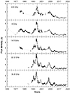 |
Fig. 1. Light curves of AGN S 0528+134 in the indicated wavelength ranges. |
Based on the data obtained at all frequency radio ranges, a harmonic analysis of the source radiation was carried out using the Schuster method (Volvach et al. 2023). As a result, harmonic components of flux density variability were identified that exceeded the level of five standard deviations (Table 2).
Periodic components of radiation variability 0528+134.
The methodology for conducting harmonic analysis is given in the appendix. An example of harmonic analysis data performed at 8 GHz is shown in Fig. 2.
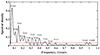 |
Fig. 2. Example of harmonic analysis data performed at 8 GHz. The horizontal line shows the 5σ level limit. |
It should be noted that we present one of the possible interpretations of the harmonic analysis data. All of the harmonic analysis data presented in Table 2 correspond to peaks in the power spectrum above the 5σ level. The most significant periods that we distinguish from the periodogram are T = 3.0, 6.4, and 12.1 years. The indicated periods have a maximum amplitude in relation to other periods. We cannot explain the 6.4 year period from a physical point of view. The period of 12.1 (Tpr) years, an average over all frequencies, can be associated with the movements of the central SMBH and accretion disc (AD). The period 3.0 is present at all frequencies in the error limits. This can be the period of the companion’s orbital motion (Torb). The choice of precessional and orbital periods is made conditionally, as it has been by all other authors of similar studies, which we mention below.
The last row of Table 2 gives the period, Tsource, in the co-ordinate system associated with the source (z = 2.07, γ = 5) through the period received by the observer, Tobs (Rieger 2007):
 (1)
(1)
A γ parameter was not obtained directly from monitoring observations. There are currently no gamma value data available for 0528+134. Its value can be estimated from a comparison of the durations of flares in different AGNs, assuming that there is a relationship between the duration of flares and value of γ factors. In S0528+134, the flares have different durations in different epochs. We assumed that the gamma factor is directly dependent on the duration of the flare. The gamma factor, γ ≈ ΔT/Δt, where Δt is the duration of the flare in years, and ΔT = 2π radian. According to observational data for the 2007 flare, γ ≈ 6.3. However, the uncertainty of this value can reach 50% (Volvach et al. 2014). We focussed on a gamma factor value of 5–10.
Other methods of determining the angle between the emission from the object and the direction towards the observer can be noted. Monitoring S5 0716+714 with the millimetre VLBI network allows us to study the internal kinematics of the jet and investigate its relationship with the observed broadband flux density variability (Rani et al. 2015). The study reveals significant non-radial motions in the jet outflow, including variations in the orientation at the sub-parsec scale of the jet, including the helical trajectories of its moving components. The individual components exhibit extreme apparent speeds as high as 37 c on parsec scales. The typical value of the apparent velocity is 20 c, but sometimes it reaches 44 c (Lister et al. 2013). In this case, the flux density will increase by an order of magnitude. The other origin of major optical/γ-ray/radio outbursts in the source seems to be related to a disturbance, such as a shock wave, propagating in the jet. Other reasons include the option of magneto-hydrodynamic instabilities (Hardee 2006).
We believe that the flares in object S 0528+134 last about a year, as in 3C 454.3, where the gamma factor value was estimated to be 5–10. We accept this value for S 0528+134. The values of the precessional and orbital periods that we have accepted are in line with the data of other authors who analyzed materials for other sources. For example, for 3C 120, the values obtained were Tpr = 12.3 years and Torb = 1.4 years (Caproni & Abraham 2004). In the source OJ 287, a period of 11.65 years was identified based on optical data (Sillanpaa et al. 1996, 1988; Pietila et al. 1999; Aller et al. 1992; Shukla & Stoner 1996). Precessional and orbital periods of 12.4 and 3.0 years have been identified in 3C 273 (Volvach et al. 2013). Thus, our choice of orbital and precessional periods in S 0528+134 seems quite natural and based on the results of many years of multi-frequency observations in the radio range. Harmonic analysis of the γ-band data also gives a value close to the precession period, but due to the limited data sample this value cannot be taken into consideration.
The relationship between the obtained values of the orbital and precessional periods can be based on Keppler’s laws for a system of binary SMBHs (Volvach et al. 2023). As a result, we have a connection between the periods and masses of the companions (m, M) and the value of the companion’s orbit, r:
 (2)
(2)
 (3)
(3)
The ratio of the masses of the companions, obtained from expressions (2) and (3), gives the value M/m ≈ 2.0, which leads to the value (Volvach et al. 2023):
 (4)
(4)
3.2. Lifetime of close binary supermassive black holes
Emission from S 0528+134 at all wavelength ranges of the electromagnetic spectrum makes a significant contribution to reducing the lifetime of this binary system. Another factor, which is related to the first one that reduces the lifetime of the system, Another factor that reduces the lifetime of the system, which is related to the first one, is the dynamic friction that arises when supermassive companions move through the dense environment of AD and accreting matter. We considered the loss of the orbital momentum of the system due to dynamic friction with the medium for the binary SMBH 3C 454.3 in the article (Volvach et al. 2021). Energy losses due to radiation in the electromagnetic spectrum for the binary S 0528+134 were considered in (Sambruna et al. 1997). The authors calculated that in the range from 1017 to 1025 Hz, using the spectral parameters S 0528+134, the bolometric luminosity of the object reaches a value of approximately Ebol ≈ 1049 erg s−1. This luminosity is provided, first, by dynamic losses in the medium in which the SMBH companions move. Therefore, we consider the main energy losses in this object to be its losses due to radiation in the entire range of the electromagnetic spectrum equal to ΔE = 1049 erg s−1.
Energy losses in the system are closely related to the lifetime of binary SMBHs, which is also determined by their energy reserves. The kinetic energy of the companions fuels the object’s bolometric luminosity. The expression for tmerge shows its relationship with the masses of the binary SMBH (M, m) and the size of the companion orbit, r (Peters 1964):
 (5)
(5)
which gives the value for S 0528+134,
 (6)
(6)
It is taken into account that M ≈ 2m. We note the strong dependence of the system’s lifetime on the radius of the companion’s orbit. To determine the three parameters (tmerge, r and M), one needs to have three equations. We have only two relations (4), (5), so it is necessary to add some more natural restrictions on the parameters of the SMBH. To these equations, one also needs to add one more thing and, accordingly, know Torb, Tpr. We can conditionally take the lifetime before the merger for the source S 0528+134 to be tmerge ≈ 2 ⋅ 105 years. Our considerations boil down to the following.
According to (5), there is a very strong dependence, in the fourth degree, of the system’s lifetime on the size of the companion’s orbit. Doubling the orbital size leads to an increase in the lifetime of 16 times. The reserves of kinetic energy of the system, which are spent on overcoming the dynamic resistance of the environment in it when the companions move in orbit, should also increase by the same amount. And if previously supermassive SMBHs moved in orbits at speeds of about (1 − 2)⋅104 km s−1, as, for example, in 3C 273 (Volvach et al. 2023), now their speed of movement should already reach tenths of the speed of light, which is physically impossible, since this must be accompanied by an unimaginable release of energy, which is not observed. On the contrary, reducing the companion’s orbit by half leads to an extremely short lifetime of about 104 years, which is unacceptable from the point of view of the probability of the existence of a significant number of bright AGNs. The companion’s orbital sizes were obtained because of tough compromises with regard to the companions’ lifetimes. Changing the lifetime of the system by two in one direction or another will lead to unrealistic values for the parameters of the orbits of the companions, taking into account the fourth degree of dependence of these parameters on the lifetime of the companions.
We obtained the value of the radius of the companion’s orbit by substituting M from relation (4) into (6) and taking the system lifetime (2 ⋅ 105 years), as well as transitions from units expressed in solar masses to grams and vice versa:
 (7)
(7)
where we get here; when the value r ≈ 2 ⋅ 1017 cm. The resulting value for the orbit of the companion S 0528+134 is the smallest of the known brightest AGNs, as is the lifetime of the system before the merger.
3.3. Estimates of the accretion disc sizes of close binary supermassive black holes
This is not surprising, since no known AGN emits as much power (1049 erg s−1) as this source. The value of M and m obtained from relations ((2), (4)) will be M ≈ 3.6 ⋅ 109 M⊙ and m ≈ 1.8 ⋅ 109 M⊙ respectively. This is a very massive, close binary system moving at high speeds inside a common AD with their common period, Torb.
We can estimate the disc dimensions using the formula with appropriate transformations (Peters 1964):
 (8)
(8)
We obtained a value for the AD radius equal to
 (9)
(9)
where, in accordance with the laws of celestial mechanics, rcentr = 1.4 ⋅ 1017 cm. The dimensions of the disc are more than an order of magnitude larger than the radii of the orbits of the companions, which rotate in the dense central regions of the AD at gigantic speeds.
Based on the values of the periods and sizes of the companion orbits, the orbital speeds are equal, Vcomp ≈ 1.7 ⋅ 104 km s−1 and Vcentr ≈ 1.0 ⋅ 104 km s−1. Behind the shock wave fronts, the directed motion of particles is transformed into chaotic motion. The plasma temperature exceeds 1010 K at the temperature threshold for the birth of electron–positron pairs, Te − p = 5 ⋅ 109 K. Thus, we have e − p plasma transforming into relativistic ‘jets’ using the SMBH rotation mechanism in its last stable orbit and electric and magnetic fields as sources of plasma acceleration. Therefore, in general, jets can form in AGNs. It can be noted that the source of the primary energy release in the system of binary SMBHs is the movement of companions through the dense medium of the AD with the speed of movement of matter equal to that in explosions of type I supernovae.
After the brightest currently known flare in the AGN S 0528+134 in 1994 and less powerful flares in 2008–2011, the angle of radiation has in recent years begun to turn away from terrestrial earthly observers due to precessional movements in the system and a narrow cone of energy emission. Changes in the gamma factor in the radio band may be insignificant, since there are no significant changes in the periods of change in the flare flux density according to the readings of harmonic analysis. The amplitude of flux density variations changes noticeably (Fig. 1). The gamma factor and the Doppler factor are related values (Bach et al. 2005). Changing the Doppler factor by a factor of two leads to a change in the flare amplitude of almost an order of magnitude, which is actually observed. Thus, at viewing angles ≤5°, the Doppler factor approaches δ ≈ 2γ (Bach et al. 2005). That is, less significant changes in the γ factor may be accompanied by larger fluctuations in the δ factor. Considering the small sample of monitoring data in recent years and the insignificant amplitudes of flux density variations, experimental errors can be significant and mask not very large changes in the periods of flux density fluctuations, and therefore the γ factor.
The found masses and sizes of the orbits of S 0528+134 (M ≈ 3.6 ⋅ 109 M⊙, m ≈ 1.8 ⋅ 109 M⊙, rcomp ≈ 2 ⋅ 1017 cm) indicate that this binary SMBH is very massive and one of the most compact among other known SMBHs, such as OJ 287, 3C 454.3, 3C 273, and AO 0235+164. The ratio of the masses of the S 0528+134 companions is 2. For massive stars in the Galaxy, this ratio of the masses of the companions is common and often turns out to be close to unity (Chini et al. 2012). Supermassive companions revolve around a common centre of gravity with the same period due to the strong gravitational interaction between them. It can be assumed that in close binary SMBHs at the stage of evolution close to merging, there can be only one AD, common to both SMBHs. When, due to dynamic friction in the environment, the distance between the SMBH orbits decreases to 0.1–1 pc, the smaller black hole loses its AD (Lobanov 2004). In this case, a binary SMBH can have one AD, which will be located near the common centre of gravity. Until this time, the companions evolve as separate structures. This process can be very lengthy, lasting many millions of years (Lobanov 2004). Kiehlmann et al. estimate the fraction of blazars that are SMBH candidates to be > 1 in 100, and thus monitoring programs covering tens of thousands of blazars could discover hundreds of SMBH candidates (Kiehlmann et al. 2024). For PKS 2131-021 in the kinetic orbital model the orbital motion changes the velocity of the emitting material in the jet relative to the observer, and hence the Doppler factor and beaming (O’Neill et al. 2022).
Taking into account the obtained sizes of the AD in a situation where it is equal to the standard α disc (Caproni & Abraham 2004), we have had = 0.07 ⋅ ad ≈ 0.07 ⋅ 1.7 ⋅ 1018 cm ≈ 1.2 ⋅ 1017 cm. It is close to the size of the companion’s orbit (rcomp = 2 ⋅ 1017 cm). This means that the orbits of the companions always lie within the dense environment of the AD. This is also true for other brightest AGN. From the above, it becomes clear that AD S 0528+134, like all brightest AGNs, may be sources of powerful X-ray and gamma radiation.
3.4. Gravitational radiation from AGN S 0528+134
From the data obtained for S 0528+134, we can calculate the rate of energy loss due to GW radiation, taking the value e = 0 (Peters 1964):
 (10)
(10)
Thus, the emission power of GWs from S 0528+134 exceeds the emission power of all known AGNs, except for 3C 454.3, which is the shortest-lived object from the category of close binary SMBHs. At the same time, it should be taken into account that S 0528+134 is located more than 2.5 times further than 3C 454.3 (Volvach et al. 2021), and therefore appears almost seven times fainter on Earth. However, in terms of bolometric luminosity, it surpasses all known AGNs. In addition, 3C 454.3 is the shortest-lived of all known AGNs. The lifetime before the merger of its SMBH is only a few tens of thousands of years (Volvach et al. 2021). To confirm that S 0528+134 is the most powerful emitter in the Universe, we refer to the fact that with a comparable flux density of γ radiation from S 0528+134 and 3C 454.3, the first of them is located significantly further away and, accordingly, has radiation power almost an order of magnitude greater. Therefore, we can consider blazar S 0528+134 to be the most powerful emitter in the Universe. In terms of the level of GW flux on the Earth’s surface, S 0528+134 is one of the promising candidates for detecting GWs from a source using International Pulsar Timing Array (IPTA) GW detectors. As result, we can also conclude that the energy reserves in bright AGNs are used to overcome dynamic friction in a dense AD medium and are converted into broadband radiation from radio to gamma.
4. Conclusions
Long-term monitoring of what is possibly the most powerful emitter in the Universe, S 0528+134, was performed at five frequencies in the radio range from 4.8 GHz to 37 GHz at the Radio Astronomy Laboratory of the Crimean Astrophysical Observatory, the Metsähovi Radio Observatory of Aalto University, the Radio Astronomy Observatory of the University of Michigan, and in the gamma-ray range at the Fermi Large Astronomical Telescope (LAT).
The evolution of powerful outbursts that have occurred at the object since its discovery in a sky survey in 1970 were investigated. Under the assumption of the hypothesis of the existence of an SMBHs in the central regions of galaxies, the main physical characteristics of binary SMBHs were obtained: the masses of the SMBH companions, the parameters of their orbits, the energy reserve of the system, and the lifetime of the object before the SMBHs’ merger. The magnitude of GWs on the Earth’s surface was calculated and the possibility of detecting them with IPTA GW detectors was considered.
Acknowledgments
We express our gratitude to the anonymous reviewer for his constructive comments during the preparation of the article. This research has made use of data from the OVRO 40-m monitoring program which is supported in part by NASA grants NNX08AW31G, NNX11A043G, and NNX14AQ89G and NSF grants AST-0808050 and AST-1109911.
References
- Aller, M. F., Aller, H. D., Latimer, G. E., & Hodge, P. 1985, ApJS, 59, 513 [NASA ADS] [CrossRef] [Google Scholar]
- Aller, M., Aller, H. D., Hughes, P., & Latimer, G. 1992, in Variability of Blazars, eds. E. Valtaoja, & M. Valtonen (Cambridge: Cambridge Univ. Press), 470, 126 [NASA ADS] [Google Scholar]
- Bach, U., Krichbaum, T. P., Ros, T., Britzen, S., & Tian, W. 2005, A&A, 43, 815 [NASA ADS] [CrossRef] [EDP Sciences] [Google Scholar]
- Baliunas, S., & Horne, J. 1986, ApJ, 302, 757 [CrossRef] [Google Scholar]
- Barning, F. 1963, Bull. Astron. Inst. Neth., 17, 22 [NASA ADS] [Google Scholar]
- Bennett, A., & Simth, F. 1962, MNRAS, 125, 75 [CrossRef] [Google Scholar]
- Bolton, J., Gardner, F., & Mackey, M. 1964, Aust. J. Phys., 17, 340 [Google Scholar]
- Caproni, A., & Abraham, Z. 2004, MNRAS, 349, 1218 [NASA ADS] [CrossRef] [Google Scholar]
- Chini, R., Hoffmeister, V. H., Nasseri, A., et al. 2012, MNRAS, 470, 831 [Google Scholar]
- Claudi, R., Bonanno, A., Ventura, R., & Bonanno, G. 2004, Commun. Asteroseismol., 145, 53 [NASA ADS] [Google Scholar]
- de Jong, M. 1967, ApJ, 150, 1 [NASA ADS] [CrossRef] [Google Scholar]
- Deeming, T. 1975, Astrophys. Space. Science, 36, 137 [NASA ADS] [Google Scholar]
- Dent, W. 1965a, Science, 148, 3676 [Google Scholar]
- Dent, W. 1965b, AJ, 70, 672 [NASA ADS] [CrossRef] [Google Scholar]
- Dent, W., & Haddock, F. 1965, Nature, 205, 487 [NASA ADS] [CrossRef] [Google Scholar]
- Edge, D., Shakeshaft, J., McAdam, W., et al. 1959, MNRAS, 68, 37 [Google Scholar]
- Ehman, J., Dixon, R., Ramakrishna, C., & Kraus, J. 1974, AJ, 79, 144 [NASA ADS] [CrossRef] [Google Scholar]
- Goss, W., Hooker, C., & Ekers, R. 2023, Joe Pawsey and the Founding of Australian Radio Astronomy (Springer), 815 [Google Scholar]
- Greenstein, J. L., & Matthews, T. 1963, Nature, 197, 1041 [NASA ADS] [CrossRef] [Google Scholar]
- Hardee, P. E. 2006, AIP Conf. Ser., 856, 57 [NASA ADS] [CrossRef] [Google Scholar]
- Hunter, S. D., Bertsch, D. L., Dingus, B. L., et al. 1993, ApJ, 409, 134 [NASA ADS] [CrossRef] [Google Scholar]
- Kiehlmann, S., de la Parra, P., Sullivan, A., & Synani, A. 2024, ApJ, submitted [Google Scholar]
- Kraus, J. 1966, Radio Science, 1, 662 [Google Scholar]
- Lanza, A., Rodono, M., & Zappala, R. 1993, A&A, 269, 351 [NASA ADS] [Google Scholar]
- Larionov, M., Gorshkov, A., & Popov, M. 1970, Astron. Tsirkulyar, 590, 3 [NASA ADS] [Google Scholar]
- Larionov, M., Gorshkov, A., Popov, M., et al. 1971, Astron. Tsirkulyar, 665, 1 [NASA ADS] [Google Scholar]
- Lister, M. L., Aller, M. F., & Aller, H. D. 2013, ApJ, 146, 120 [Google Scholar]
- Lobanov, A. 2004, ArXiv e-prints [arXiv:astrp-ph/0412416v1] [Google Scholar]
- Lomb, N. 1976, Astrophys. Space Sci., 39, 447 [NASA ADS] [CrossRef] [Google Scholar]
- Mukherjee, R., Dingus, B. L., Gear, W. K., et al. 1996, ApJ, 470, 831 [NASA ADS] [CrossRef] [Google Scholar]
- O’Neill, S., Kiehlmann, S., & Readhead, A. 2022, ApJ, 926, L35 [CrossRef] [Google Scholar]
- Peters, P. 1964, Phys. Rev. B, 136, 1224 [Google Scholar]
- Pietila, H., Takalo, L. O., Tosti, G., et al. 1999, A&A, 345, 760 [Google Scholar]
- Pohl, M., Reich, W., Krichbaum, T. P., et al. 1995, A&A, 303, 383 [NASA ADS] [Google Scholar]
- Rani, B., Krichbaum, T. P., Marscher, A. P., et al. 2015, A&A, 578, A123 [NASA ADS] [CrossRef] [EDP Sciences] [Google Scholar]
- Richards, J. L., Max-Moerbeck, W., Pavlidou, V., et al. 2011, ApJS, 194, 29 [Google Scholar]
- Rieger, F. 2007, Astrophys. Space Sci., 309, 271 [NASA ADS] [CrossRef] [Google Scholar]
- Roberts, D., Lehar, J., & Dreher, J. 1987, ApJ, 93, 968 [CrossRef] [Google Scholar]
- Sambruna, R. M., Urry, C. M., Maraschi, L., et al. 1997, ApJ, 474, 639 [NASA ADS] [CrossRef] [Google Scholar]
- Scargle, J. 1982, ApJ, 263, 835 [NASA ADS] [CrossRef] [Google Scholar]
- Schmidt, M. 1963, Nature, 197, 1040 [Google Scholar]
- Scott, P., & Ryle, M. 1961, MNRAS, 125, 389 [CrossRef] [Google Scholar]
- Sholomitsky, G. 1965, Inf. Bull. Variable Stars, 83, 1 [NASA ADS] [Google Scholar]
- Shukla, H., & Stoner, R. 1996, ApJS, 106, 41 [NASA ADS] [CrossRef] [Google Scholar]
- Sillanpaa, A., Haarala, S., Valtonen, M. J., et al. 1988, ApJ, 325, 628 [NASA ADS] [CrossRef] [Google Scholar]
- Sillanpaa, A., Takalo, L. O., Pursimo, T., et al. 1996, A&A, 305, 17 [Google Scholar]
- Vityazev, V. 1996, Astron. Astrophys. Trans., 11, 159 [NASA ADS] [CrossRef] [Google Scholar]
- Volvach, A., Volvach, L., & Larionov, M. 2013, Astron. Rep., 57, 34 [NASA ADS] [CrossRef] [Google Scholar]
- Volvach, A., Volvach, L., & Larionov, M. 2014, Astron. Rep., 58, 71 [NASA ADS] [CrossRef] [Google Scholar]
- Volvach, A., Volvach, L., & Larionov, M. 2021, A&A, 648, A27 [NASA ADS] [CrossRef] [EDP Sciences] [Google Scholar]
- Volvach, A., Volvach, L., & Larionov, M. 2023, Galaxies, 11, 96 [NASA ADS] [CrossRef] [Google Scholar]
- Wall, J., & Peacock, J. 1985, MNRAS, 216, 173 [NASA ADS] [CrossRef] [Google Scholar]
- Wall, J. V., Wright, A. E., & Bolton, J. G. 1976, Aust. J. Phys., 29, 123 [NASA ADS] [CrossRef] [Google Scholar]
- Wen, L., Levine, A., Corbet, R., & Bradt, H. 2006, ApJS, 163, 372 [NASA ADS] [CrossRef] [Google Scholar]
- Zhang, Y. F., Marscher, A. P., Aller, H. D., et al. 1994, ApJ, 432, 91 [NASA ADS] [CrossRef] [Google Scholar]
Appendix A: The harmonic analysis
One of the power spectrum estimates often used in practice is the LS spectrum (Wen et al. 2006; Claudi et al. 2004; Lanza et al. 1993), the mathematical apparatus of which was developed in (Barning 1963; Lomb 1976; Scargle 1982). Its construction is based on the approximation of a time series by the sum of harmonic functions using the least squares method. The advantage of the LS spectrum is the exponential distribution of white noise periodogram samples. On the other hand, the main disadvantage is the lack of analytical connection between the power spectrum estimate and its true value.
Another method of analysis, free from this drawback, is the calculation of the Schuster periodogram D(w), associated with the true power spectrum g(w) and spectral window W(w) by the fundamental relation (Deeming 1975; Vityazev 1996):
 (A.1)
(A.1)
This relationship made it possible to ’clean up’ the spectrum, i.e. to remove unnecessary peaks associated with a finite and non-uniformly spaced time grid, as well as false maxima due to noise. To "clean" the spectrum, we decided to use the CLEAN method, which was originally developed for processing two-dimensional maps obtained during aperture synthesis. Later, it began to be used in spectral analysis of one-dimensional time series (Roberts et al. 1987). The CLEAN technique associated with the successive subtraction of all significant maxima from the ’dirty’ spectrum. Each subtracted spectral peak is defined by its complex amplitude, frequency, and spectral window, which depends on the distribution of the data over time. The procedure for "cleaning" the spectrum lasts until there is not a single peak left in the "dirty" spectrum whose value exceeds a certain threshold level, depending on the probability of detecting a signal in the noise. This level can be determined by knowing the type of distribution of samples of the noise periodogram (Scargle 1982). It is known (Scargle 1982; Baliunas & Horne 1986). However, in the case of an uneven time grid, it is impossible to obtain a strict expression for this distribution. Some authors [Baliunas, Horne, 1986] have obtained empirical formulas for certain uneven series, but they cannot be considered universal, since for each specific series the distribution in question will be specific. Therefore, in order to obtain the signal detection threshold in noise, in this work, for each processed series, the characteristic distribution of white noise periodogram counts is calculated for it. All subtracted peaks give a clean spectrum, devoid of false maxima and noise. The spectrum is cleaned until there are no peaks in the ’dirty’ spectrum that exceed a certain threshold level, determined by the probability of detecting a signal in the noise. With the help of spectral analysis algorithms, we revealed variations with different periods of the light curves of S 0528+134. The data obtained using the CLEAN technique are presented in Table 2 for all given frequencies in the radio and optical wavelength ranges.
All Tables
All Figures
|
Fig. 1. Light curves of AGN S 0528+134 in the indicated wavelength ranges. |
| In the text | |
|
Fig. 2. Example of harmonic analysis data performed at 8 GHz. The horizontal line shows the 5σ level limit. |
| In the text | |
Current usage metrics show cumulative count of Article Views (full-text article views including HTML views, PDF and ePub downloads, according to the available data) and Abstracts Views on Vision4Press platform.
Data correspond to usage on the plateform after 2015. The current usage metrics is available 48-96 hours after online publication and is updated daily on week days.
Initial download of the metrics may take a while.