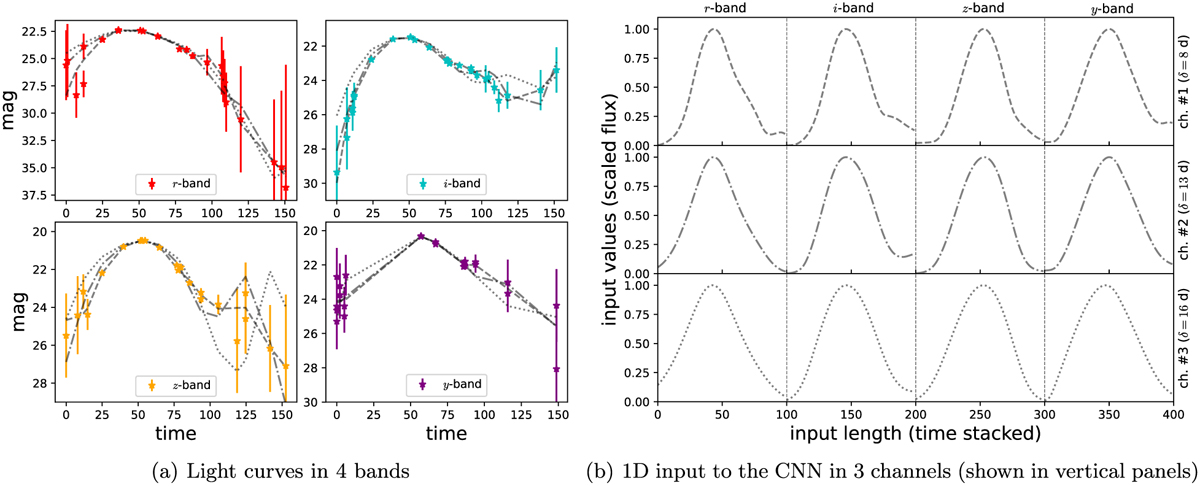
(a) Blended light curves of a typical unresolved system are shown in the left panel across four LSST bands. We adopt LSST-like cadence and noise to generate mock light curves (as detailed in Sect. 3.3). Data processing begins by smoothing these light curves using different smoothing scales. The grey curves, delineated with dashed, dash-dotted, and dotted line styles, represent the smoothed light curves corresponding to smoothing scales of 8, 13, and 16 days, respectively. Subsequently, we convert the smoothed magnitudes into fluxes and sample the light curves on a predefined set of epochs, kept fixed for each band. For simplicity, we opt for 100 epochs with 1 day spacing, starting from the initial observation epoch (set as t = 0), for all the bands. We then normalise every light curve separately by scaling the fluxes in the range [0,1]. (b) Finally, for each smoothing scale, we stack the normalised flux-versus-time light curves corresponding to the four bands side by side, thereby recasting the data into an array of 400 in length. Subsequently, we arrange three such arrays – corresponding to the three choices of smoothing scale – into three channels. Consequently, the final data size for each system becomes (400,3), as depicted in the right panel. This sample of data, of fixed size, is then fed into the CNNs.