| Issue |
A&A
Volume 690, October 2024
|
|
|---|---|---|
| Article Number | A295 | |
| Number of page(s) | 11 | |
| Section | Stellar atmospheres | |
| DOI | https://doi.org/10.1051/0004-6361/202449850 | |
| Published online | 17 October 2024 | |
Infrared surface brightness technique applied to RR Lyrae stars from the solar neighborhood★
1
Universidad de Concepción, Departamento de Astronomía,
Casilla 160-C,
Concepción,
Chile
2
Nicolaus Copernicus Astronomical Center, Polish Academy of Sciences,
Bartycka 18,
00-716
Warszawa,
Poland
3
Leibniz-Institut für Astrophysik Potsdam (AIP),
An der Sternwarte 16,
14482
Potsdam,
Germany
4
LESIA, Observatoire de Paris, Université PSL, CNRS, Sorbonne Université, Université Paris Cité,
5 place Jules Janssen,
92195
Meudon,
France
5
Université Côte d’Azur, Observatoire de la Côte d’Azur, CNRS, Laboratoire Lagrange,
06304
Nice Cedex 4,
France
6
Astronomisches Institut, Ruhr-Universität Bochum,
Universitätsstrasse 150,
44801
Bochum,
Germany
7
Instituto de Astronomía, Universidad Católica del Norte,
Avenida Angamos 0610,
Antofagasta,
Chile
★★ Corresponding author; This email address is being protected from spambots. You need JavaScript enabled to view it.
Received:
4
March
2024
Accepted:
1
August
2024
Abstract
Context. The Baade-Wesselink (BW) method, also known as the pulsation parallax method, allows us to estimate distances to individual pulsating stars. Accurate geometric parallaxes obtained by the Gaia mission serve us in the calibration of the method and in the determination of its precision. This method also provides a way of determining mean radii of pulsating stars.
Aims. The main aim of this work is to determine the scatter and possible dependence of p-factors of RR Lyrae stars on their pulsation periods. The secondary objective is to determine the mean radius-period relations for these stars.
Methods. Our calibrations for RR Lyrae stars are based on photometric data gathered at the Cerro Murphy Observatory and parallaxes from the Data Release 3 of the Gaia space mission. We obtained spectroscopic data specifically for this project using high-resolution spectrographs. We used the infrared surface brightness (IRSB) version of the method that relies on a surface brightness-color relation that is dependent on the (V − K) color. It allows us to estimate stellar angular diameters, while tracing variations of the stellar radius using measurements of the stellar radial velocity obtained from spectroscopy. We present results based on four different empirical surface brightness-color relations, with three relations for dwarfs and subgiants and one for classical Cepheids.
Results. We present our calibration of projection factors and determination of the mean radii for nine Galactic RR Lyrae stars. We obtained a spread of p-factors of around 0.07–0.08 for our sample of RR Lyrae stars from the solar neighborhood. However, depending on a given SBCR, we also found relations between the p-factor and the pulsation period for RRab stars with a root mean square (rms) scatter around the relation of around 0.05, but with relatively large uncertainty on the relation parameters. We also present relations between the mean radius and period for RR Lyrae pulsating in the fundamental mode with an rms scatter around the relation of 0.012 R⊙. We observe a clear offset between p-factors obtained using the IRSB technique (with a mean p value between 1.39 and 1.45) and values inferred using the SPIPS tool. This confirms that different implementations of the BW method are sensitive to various components of the p-factor. On the other hand, we obtain a similar scatter for p, as observed in a previous study based on the SPIPS tool. Our period-radius relations are in a good agreement with both the inference based on SPIPS and theoretical predictions.
Key words: stars: distances / stars: oscillations / stars: variables: RR Lyrae / infrared: stars
Based on excerpts from the PhD thesis (Zgirski 2022).
© The Authors 2024
 Open Access article, published by EDP Sciences, under the terms of the Creative Commons Attribution License (https://creativecommons.org/licenses/by/4.0), which permits unrestricted use, distribution, and reproduction in any medium, provided the original work is properly cited.
This article is published in open access under the Subscribe to Open model. This email address is being protected from spambots. You need JavaScript enabled to view it. to support open access publication.
1 Introduction
The Baade-Wesselink (BW) method (Baade 1926; Wesselink 1946), originally proposed as a testing tool of the pulsation hyphothesis for Cepheids, allows for the determination of mean radii and geometric distances of individual radially pulsating stars. Conceptually, the foundation of the method lies in the inference based on the analysis of variations of both the stellar radius and the angular diameter. The two parameters are connected via a simple geometric relation:
![Mathematical equation: $\[\theta(\phi)=\frac{2 R(\phi)}{r}=\frac{2\left[R_0+\Delta R(\phi)\right]}{r}=2 \varpi\left[R_0+\Delta R(\phi)\right],\]$](/articles/aa/full_html/2024/10/aa49850-24/aa49850-24-eq1.png) (1)
(1)
where θ is the angular diameter of a star at a given pulsation phase ϕ, R − the stellar radius, r is the distance, and ϖ − is the corresponding parallax. R0 is the radius of the pulsator corresponding to (an arbitrarily chosen) ϕ = 0, while ΔR corresponds to its variations in time.
Variations of the stellar radius may be traced using spectroscopic measurements of radial velocities:
![Mathematical equation: $\[\Delta R(\phi)=-\int p\left[v_r(\phi)-v_{r, 0}\right] d \phi,\]$](/articles/aa/full_html/2024/10/aa49850-24/aa49850-24-eq2.png) (2)
(2)
where vr(ϕ) is the measured radial velocity, vr,0 is the systemic (average) radial velocity obtained from the integration of the radial velocity curve over the whole phase, and p is a projection factor (also known as the p-factor). It is a parameter that translates apparent radial velocities into stellar pulsation velocities that correspond to the derivative of the stellar radius. A proper calibration of the p-factor and its dependence on intrinsic stellar parameters are essential for accurate distance determinations based on this method. Nardetto et al. (2007) divided the p-factor into a product made up of the following components:
p0, the geometrical projection factor, which is an integral of the pulsation velocity of the stellar line-forming region (observed using spectroscopy) projected onto the line of sight and weighted by the stellar surface brightness.
fgrad, a ratio of the gas velocity of the photosphere (observed using interferometry or photometry) and the gas velocity of the line-forming region.
fo–g, a ratio of the pulsation velocity and the gas velocity of the photosphere.
The BW method was used before most notably for classical Cepheids. Among works published during the previous decade, Storm et al. (2011) calibrated a relation between Cepheids’ p-factors and pulsation periods. The authors also established period-luminosity (PL) relations for classical Cepheids based on their BW distances. Gieren et al. (2018) investigated the dependence of Cepheids’ PL relations on metallicity through the determination of distances to single stars in the Milky Way and the two Magellanic Clouds based on the dependence of p-factor on pulsation period from Storm et al. (2011). A lot of effort has been put to calibrate the method for Cepheids in order to obtain distances with the precision of a few percent. However, Trahin et al. (2021) found no correlation between p-factors and the pulsation period or the metallicity for a sample of 63 classical Cepheids from the Milky Way based on their Gaia parallaxes. The authors obtained a large scatter (around 12%) of values of projection factors, which could indicate larger complexity behind the simple reduction of the problem to one calibrated parameter.
Meanwhile, another species of classical pulsators, RR Lyrae stars, which are significantly fainter than classical Cepheids, have also been considered as important distance indicators. With ages greater than 10 Gyr (Catelan & Smith 2015), they trace a different (old) stellar population and can be found in (sub-)systems where classical Cepheids are not present, such as globular clusters or dwarf spheroidal galaxies. They have been utilized in distance determinations since the work of Shapley (1918), where the size of the Milky Way and the position of the Sun in the Galaxy were estimated by the author based on a study of RR Lyrae stars in a number of globular clusters. In the context of the cosmic distance ladder, where long-range distance determination methods are calibrated using more accurate short-range methods, RR Lyrae stars are one of the calibrators of the tip of the red giant branch technique used in the determination of the most important cosmological parameter: the Hubble constant (Freedman 2021).
The BW method for RR Lyraes provides an independent alternative to distance determinations to old stellar systems that are based on period-luminosity(-metallicity) relations for these stars (e.g. Pietrzyński et al. 2008; Szewczyk et al. 2008; Szewczyk et al. 2009; Karczmarek et al. 2015, 2017; Zgirski et al. 2023). Distance determinations to individual stars based on the well-calibrated BW method could yield much more accurate spatial distributions of pulsators than what is possible to obtain using period-luminosity relations (e.g., Jacyszyn-Dobrzeniecka et al. 2017). In the face of the problematic calibration of p-factors for classical Cepheids, a question has arisen as to whether RR Lyraes could provide less scattered and more predictable values of the factor. In principle, RR Lyrae stars are challenging for the BW analysis as their pulsation periods are short and their periods may change significantly over many pulsation cycles (Catelan & Smith 2015; Jurcsik et al. 2012). The light curves of a significant number of these stars undergo the Blazhko modulation (Blažko 1907; Jurcsik et al. 2018). Thus, RR Lyrae stars require data collection during similar epochs in temporally compact observing campaigns.
In the 1980s and early 1990s, a series of works devoted to the estimation of mean absolute magnitudes (bolometric and visual) of field Galactic RR Lyrae stars and their dependence on metallicity was published. Stellar angular diameters were estimated based on the notion of the visual surface brightness, SV (Wesselink 1969, reevaluation by Manduca & Bell 1981), a quantity that depends on the effective stellar temperature and the bolometric correction in the V band.
In one of these series of papers (Carney & Latham 1984; Jones et al. 1987a,b, 1988a,b, 1992; Jones 1988; Carney et al. 1992), the authors assumed values of p-factor from between p = 1.30 and 1.36. In their second paper (Jones et al. 1987a), they introduced an analysis that relied on estimating the stellar apparent bolometric magnitude and effective temperature using the (V − K) color. The authors estimated that this specific method should yield an accuracy of determination of the absolute magnitude of an RR Lyrae star of about 0.1 mag. In the same work, the authors recognized the influence of shock waves appearing in the atmospheres of RR Lyrae variables (Hill 1972), which manifested itself as a bump near the minimum brightness in the V- light curve, and the corresponding anomalous measurements of radial velocity. All this resulted in a poor correspondence between changes of radius derived from the radial velocity curve and changes in the angular diameter derived from spectroscopy for pulsation phases affected by the shock. Such phase intervals, apparently affected by shocks, were rejected in that and the following works.
In another series (Cacciari et al. 1989a, 1989b; Clementini et al. 1990), the authors used (V − I) and (V − R) colors to derive angular diameters of stars. They assumed p = 1.36. Then, Liu & Janes (1990a) performed a similar analysis as Jones et al. (1987a) and, assuming p = 1.32, they derived absolute magnitudes of 13 field RR Lyrae stars. In their next paper (Liu & Janes 1990b), they determined absolute magnitudes of four stars from the globular cluster M 4.
In yet another series of papers (Fernley et al. 1989, 1990a,b; Skillen et al. 1989, 1993), a different (but qualitatively similar) approach was taken than that derived from the work of Manduca & Bell (1981). Specifically, this is the infrared (IR) flux method of Blackwell & Shallis (1977) that utilizes the well-covered ultraviolet, optical, and near-infrared (NIR) photometry for the purpose of determination of angular diameter at a given pulsation phase. The authors calibrated mean absolute magnitude-metallicity dependencies for field Galactic RR Lyrae stars in the V and K bands. They used p = 1.33 and noted its 3% uncertainty by comparing their results with those of other researchers.
Storm et al. (1994a) estimated BW distances to globular clusters M 5 and M 92 based on the analysis of two RR Lyrae stars in each of the clusters. The authors also relied on the (V − K) color and stellar atmosphere models in their estimation of stellar angular diameters. They applied p = 1.30. In another work, Storm et al. (1994b) performed the BW analysis of the RR Lyrae star V9 from the globular cluster 47 Tucanae. In their distance determination, they assumed p = 1.36. The authors also derived stellar masses and absolute magnitudes in the V and K bands in both works.
More recently, Jurcsik et al. (2017) applied the BW method to determine distances to 26 RR Lyrae stars from the globular cluster M 3 based on the dependence of effective temperature and log g on the optical color (V − I) from atmospheric models of Castelli & Kurucz (2003). The authors applied p = 1.35, as modeled by Nardetto et al. (2004). In a later work, Jurcsik & Hajdu (2017b) studied the BW method for Blazhko RR Lyrae stars from M 3. They showed that distances derived to these stars are not reliable as there is a large discrepancy between the changes of the angular diameter and radius of a Blazhko star. Obtained distances varied with different modulation phases.
Since Gaia parallaxes of stars from the Milky Way became available for the community, they have been providing an excellent opportunity for semi-phenomenological and phenomenological determinations of p-factors of the Galactic RR Lyraes with accuracy much higher than ever before. Bras et al. (2024) determined p-factors for 17 RR Lyrae stars based on Gaia DR3 parallaxes using the SPIPS code (Mérand et al. 2015) that relies on the analysis of radial velocities, multiband photometry, and stellar atmosphere models. The authors obtained a mean p = 1.236 ± 0.025 and the scatter of p-factors of σ ≈ 7%.
As noticed in the literature (e.g., Gieren et al. 2013), p-factor values depend on implementation of the BW method. It certainly hints the complexity of this parameter. It’s different physical components are not easy to split observationally in an explicit way that gives coherent results for different approaches to the method. It suggests that different implementations of the BW method do weight or highlight the different components assembling the p-factor in a different way, meaning that each particular implementation of the method requires its own specific calibration of the p-factor and its hypothetical dependence on the pulsation period.
In this work, we present determinations of p-factors using the NIR surface brightness technique. We compare the results with the recent determinations of Bras et al. (2024) relying on the different implementation of the BW method. Relying on the state-of-the-art Gaia parallaxes, the method also allows us to obtain an accurate determination of the radius of a RR Lyrae star. It is one of the most fundamental parameters that constrains stellar effective temperatures, gravity, and masses in theoretical models. We derived period-radius (PR) relations that serve as a sanity check of our inference and are easy to compare with theoretical predictions, such as those of Marconi et al. (2005, 2015).
Our long-term project includes photometric and spectroscopic observations of hundreds of different species of Galactic variable stars, important distance indicators. However, in this work we present our IR surface brightness (IRSB) analysis for RR Lyrae stars with the densest coverage of their light and radial velocity curves to date. All of these stars are at distances up to 1.4 kpc with their parallaxes determined accurately based on data from the Gaia space mission. We expect to analyze a larger sample of RR Lyraes, with the aim of the calibration of the period-luminosity-metallicity relations and the Baade-Wesselink method, after gathering more datapoints in the course of our observing campaigns. The determination of p-factors and mean radii for nine RR Lyrae stars shown here allows us to present and test our method, and draw initial conclusions based on the first calibration of the IRSB technique for field RR Lyrae stars from the solar neighborhood that is based on accurate parallaxes. This technique does not rely on stellar atmosphere models, but empirically calibrated surface brightness-color relations instead.
2 The IRSB technique
The (near-)infrared surface brightness (IRSB) technique is a specific implementation of the BW method that relies on the notion of the visual surface brightness, as defined by Barnes & Evans (1976):
![Mathematical equation: $\[F_V=4.2207-0.1 V_0-0.5 \log \theta,\]$](/articles/aa/full_html/2024/10/aa49850-24/aa49850-24-eq3.png) (3)
(3)
where V0 is the dereddened V-band magnitude. Alternatively, another definition of the visual surface brightness may be found in the literature:
![Mathematical equation: $\[S_V=V_0+5 \log \theta.\]$](/articles/aa/full_html/2024/10/aa49850-24/aa49850-24-eq4.png) (4)
(4)
Having an estimation of the surface brightness, we may determine the angular diameter. In the literature, we may find many different surface brightness-color relations (SBCRs), typically calibrated on the basis of interferometric measurements.
In their, original work, Barnes & Evans studied phenomenological relations between FV and different optical colors. Out of all studied combinations, the dependence of the surface brightness on the (V − R) color yielded the smallest scatter. The authors also found that the relation depends very little on the reddening.
An NIR SBCR for classical Cepheids was studied by Welch (1994). The author found even smaller scatter around the relation based on the (V − K) color than in the case of colors based on optical bands. As argued in that work, SBCRs based on bluer optical bands, namely, U and B, are more strongly affected by line blanketing and surface gravity. The long wavelength baseline of the (V − K) color ensures good temperature sensitivity.
Fouqué & Gieren (1997) established improved NIR surface brightness-color relations for classical Cepheids (using V − K and also J − K as surface brightness indicators) based on a larger number of interferometrically measured angular diameters of giants and supergiants, which had become available in the literature after 1994. They applied their FV vs. (V − K) calibration to a significant number of Cepheids which are members of Galactic open clusters (Gieren et al. 1997) which clearly demonstrated the superiority of the (V − K) color index over optical colors as a surface brightness indicator. Using this on a larger sample of Milky Way Cepheids, they established a K-band PL relation which, compared to the corresponding LMC Cepheid relation, yielded an LMC true distance modulus of 18.46 (Gieren et al. 1998) which is very close to the modern canonical LMC distance derived from late-type eclipsing binaries (Pietrzyński et al. 2019).
Since then, a number of works devoted to calibrations of SBCRs based on the (V − K) color for different stellar luminosity classes have appeared. Although no SBCR has been calibrated for the horizontal branch stars such as the RR Lyrae stars, these relations depend only slightly on gravity, as shown, for instance, by Di Benedetto (2005). They are also practically independent of metallicity and depend only very slightly on the reddening (Thompson et al. 2001; Pietrzyński et al. 2019). In our work, we applied four literature SBCRs and we compare results obtained on their basis:
Kervella et al. (2004a) established a relation for dwarfs and subgiants based on interferometry, FV(Dwar f) = (3.9618 ± 0.0011) − (0.1376 ± 0.0005)(V − K)0.
Kervella et al. (2004b) provide a SBCR for classical Cepheids, Fv(Ceph.) = (3.9530 ± 0.0006) − (0.1336 ± 0.0008)(V − K)0.
Graczyk et al. (2021) report a relation for dwarfs and subgiants based on Gaia EDR3 parallaxes and analysis of eclipsing binaries,
![Mathematical equation: $\[S_V=2.521+1.708 \times(V-K)_0-0.705 \times (V-K)_0^2+0.623 \times(V-K)_0^3-0.239 \times(V-K)_0^4+0.0313 \times (V-K)_0^5\]$](/articles/aa/full_html/2024/10/aa49850-24/aa49850-24-eq5.png) .
.Salsi et al. (2021) give a relation for late-type (F5/K7) sub-giants and dwarfs based on interferometry: FV = (−0.1404 ± 0.0014)(V − K)0 + (3.9665 ± 0.0025).
The relations provided by Graczyk et al. (2021) and Salsi et al. (2021) are already compatible with the 2MASS system. Also, Kervella et al. (2004a, 2004b) report relations with the K band corresponding to the NIR SAAO photometric system. We transformed the K2MASS band into KS AAO using transformation equations given in the work of Koen et al. (2007). The relation from Kervella et al. (2004b) is the only one among those applied that was calibrated for an explicitly non-matching luminosity class as a sanity check of our analysis. As stated above, such relations should not be significantly dependent on gravity and metallicity.
The presented SBCRs have different (V − K) color validity domains, depending on the spans of colors of their calibrating stars. When it comes to stars from our sample, their minimum (V − K) color is between 0.41 mag and 0.89 mag and their maximum (V − K) color is between 1.05 and 1.48 mag. In the case of the relations by Kervella et al. (2004a) and Graczyk et al. (2021), we are in the corresponding validity domains; namely, the above colors are in the span of colors of calibrators of SBCRs (Fig. 5 in Kervella et al. 2004b and Fig. 9 in Graczyk et al. 2021 works). In the case of the SBCR of Kervella et al. (2004b), as shown in Fig. 5 of that work, the validity domain corresponds to the (V − K) from the (1; 2.3) interval. When it comes to the SBCR of Salsi et al. (2021), the corresponding validity domain is also (V − K) ∈ (1; 2.3), as given in Table 5 therein. For the most part, we are not in the validity domain in these two latter cases.
In order to obtain a continuous course of the radial velocity curve and V- and K-band magnitude measurements at the same phase, we obtained the radial velocity curves and V-band light curves using Akima splines (Akima 1970, implementation in the Python package of SciPy by Virtanen et al. 2020). Akima splines are piecewise functions made out of cubic polynomials and we chose them instead of fitting Fourier series because they do not oscillate in gaps between data points. We performed interpolations between bins where each bin’s value is an average of nearby datapoints. While the Akima spline is generally not a periodic function, we applied the interpolating algorithm for three courses of data, namely, for the span of phases ϕ ∈ [−1, 2]. We then determine (V − K) color for each K-band observation epoch and integrate the radial velocity curve. The phase zero point corresponds to the highest brightness in the V-band. For each value of the integral, the corresponding V-band magnitude and (V − K) color were taken. Thus, we were able to fit a relation between the estimated values of angular diameters and values of the integral:
![Mathematical equation: $\[\theta(x)=p \varpi x+\theta_0,\]$](/articles/aa/full_html/2024/10/aa49850-24/aa49850-24-eq6.png) (5)
(5)
where x = −2 ∫[vr(ϕ) − vr,0]dϕ. The slope of such relation is a product of the p-factor and the stellar parallax while the intercept corresponds to the angular diameter for ϕ = 0.
Following a similar analysis perfomed previously for classical Cepheids (e.g. Storm et al. 2004), we performed linear fits of θ(x) relations based on the linear bisector (Isobe et al. 1990). This method finds a line that bisects two linear ordinary least-squares fits OLS(X|Y) and OLS(Y|X).
In addition to the above slope and intercept of the fit, we were able to estmate the mean radius of an analyzed star:
![Mathematical equation: $\[\langle R\rangle=\frac{\theta_0}{2 \varpi}+\langle\Delta R\rangle=\frac{\theta_0}{2 \pi}-p \int_0^1 \int_0^\phi\left[v_r\left(\phi^{\prime}\right)-v_{r, 0}\right] d \phi^{\prime} d \phi.\]$](/articles/aa/full_html/2024/10/aa49850-24/aa49850-24-eq7.png) (6)
(6)
The undoubted advantage of the IRSB method is its weak dependence on the reddening. Assuming a linear form of SBCR, we may analitically trace the propagation of the E(B − V) error and its influence on derived angular diameters and thus p-factors and stellar radii. If we consider the SBCR in the following linear form:
![Mathematical equation: $\[F_V=\alpha+\beta(V-K)_0.\]$](/articles/aa/full_html/2024/10/aa49850-24/aa49850-24-eq8.png) (7)
(7)
Based on Eq. (3) and the above assumption, we may show that any additional reddening ΔE(B − V) that affects our photometry scales the derived angular diameter as:
![Mathematical equation: $\[s=\frac{\theta^{\prime}}{\theta}=10^{2 R_v \Delta E(B-V)\left[0.1-\beta\left(1-\frac{A_K}{\lambda_V}\right)\right]}\]$](/articles/aa/full_html/2024/10/aa49850-24/aa49850-24-eq9.png) (8)
(8)
where θ′ is the angular diameter resulting from photometry affected by the additional reddening of ΔE(B − V), AV is the total extinction in the V band, AK is the total extinction in the K band, and ![Mathematical equation: $\[R_V=\frac{A_V}{E(B-V)}\]$](/articles/aa/full_html/2024/10/aa49850-24/aa49850-24-eq10.png) is the reddening law. When fitting relation (5), any shifts in reddening will effectively scale the whole ordinate axis, while ϖ and x stay the same. The following ratios correspond to each other as:
is the reddening law. When fitting relation (5), any shifts in reddening will effectively scale the whole ordinate axis, while ϖ and x stay the same. The following ratios correspond to each other as:
![Mathematical equation: $\[s=\frac{\theta^{\prime}}{\theta}=\frac{p^{\prime}}{p}=\frac{\theta_0^{\prime}}{\theta_0}=\frac{\langle R\rangle^{\prime}}{\langle R\rangle},\]$](/articles/aa/full_html/2024/10/aa49850-24/aa49850-24-eq11.png) (9)
(9)
where primed quantities all correspond to values derived based on photometry affected by the additional reddening. By plugging RV = 3.1 and ![Mathematical equation: $\[\frac{A_K}{A_V}=0.117\]$](/articles/aa/full_html/2024/10/aa49850-24/aa49850-24-eq12.png) (Cardelli et al. 1989) into Eq. (8) and using the SBCR of, for instance, Kervella et al. (2004a), where β = −0.1376, we obtain:
(Cardelli et al. 1989) into Eq. (8) and using the SBCR of, for instance, Kervella et al. (2004a), where β = −0.1376, we obtain:
![Mathematical equation: $\[s=10^{0.133 \Delta E(B-V)}.\]$](/articles/aa/full_html/2024/10/aa49850-24/aa49850-24-eq13.png) (10)
(10)
For example, any error in the reddening estimation of ΔE(B − V) = 0.1 mag would correspond to s = 1.031 and would result in the shift of p of up to 0.05 for p < 1.61. Since field RR Lyrae stars analyzed in this work populate the Galactic halo, a more realistic1 reddening uncertainty would be ΔE(B − V) = 0.02 mag. This corresponds to the scaling factor of s = 1.006. For such a value, p < 1.62 could be falsified by a wrong estimation of the reddening by less than 0.01 and ⟨R⟩ = 6R⊙ would be shifted by 0.036R⊙.
3 Data
All data adopted for this project, both photometric and spectroscipic, were gathered during simultaneously performed observing runs in order to ensure the proper phasing of data points using identical time zero points and periods.
For the purpose of this work, we collected V- and K-band magnitudes as well as the radial velocity measurements of nine non-Blazkho RR Lyrae stars from the solar neighborhood. Eight stars from the sample are RRab stars while one of them (AE Boo) is a first-overtone pulsator.
Our determinations of radial velocities relied on high-resolution spectroscopy (R > 40000) obtained for the purpose of this project using the HARPS (Mayor et al. 2003), FEROS (Kaufer et al. 1999), CORALIE (Queloz et al. 2000), and UVES (Dekker et al. 2000) spectrographs located at La Silla and Paranal observatories in Chile between 2016 and 2022. The spectroscopic data were reduced using dedicated pipelines from ESO; except in the case of FEROS data, where we used the CERES pipeline (Brahm et al. 2017). We performed measurements of radial velocities using the RaveSpan code (Pilecki et al. 2012). Measurements based on both the cross-correlation function (CCF) and the broadening function (BF, Rucinski 2002), both modeled using a Gaussian, yield virtually the same values of radial velocities. The typical uncertainty of determination of radial velocities is about 200 m/s.
Our NIR light curves were already presented in the work on period-luminosity-metallicity relations for Galactic RR Lyrae stars (Zgirski et al. 2023). They were obtained using the 0.8 m IRIS telescope located at the Cerro Murphy Observatory (OCM) in Chile and equipped with a NIR camera with a HAWAII-1 detector (Hodapp et al. 2010; Watermann 2012), the Ks- band is very similar to its counterpart from the Two Micron All Sky Survey (2MASS) system (Skrutskie et al. 2006). We obtained optical V-band photometry using a 0.4 m Vysos 16 telescope (Reipurth et al. 2004), with an SBIG STL-6303 camera and a filter wheel including BV filters, located at the same observatory. We calibrated the photometry using a dedicated reduction pipeline (Watermann 2012) based on IRAF (Tody 1986), SExtractor (Bertin & Arnouts 1996), and SCAMP (Bertin 2006). We also used our custom aperture photometry pipeline based on Astropy (Astropy Collaboration 2013) and DAOPHOT (Stetson 1987). While the K-band photometry was tied to the 2MASS sytem based on the catalog of Cutri et al. (2003), the V-band photometry was standardized onto the Johnson-Kron-Cousins system using magnitudes of comparison stars from the Gaia synthetic photometry catalog (Gaia Collaboration 2023).
In order to resolve p-factors from the fitted pϖ slopes of our fitted relations, we adopted Gaia DR3 parallaxes (Gaia Collaboration 2021) with the corrections drawn from Lindegren et al. (2021). As shown in our previous work devoted to period-luminosity relations (Zgirski et al. 2023), our calibration of absolute luminiosities of RR Lyrae stars from the solar neighborhood based on these parallaxes is coherent with the Large Magellanic Cloud distance that is based on detached eclipsing binaries of Pietrzyński et al. (2019), which proves their accuracy.
Table 1 lists our sample of Galactic RR Lyrae stars studied in this work together with pulsation periods, parallaxes, and metallicities of individual stars. Figure 1 presents light curves and a radial velocity curve for an exemplary RR Lyrae star from our sample and the whole collection of plots is available in the electronic form on Zenodo.
For the purpose of our analysis, just like in our previous work devoted to NIR period-luminosity relations for RR Lyrae stars (Zgirski et al. 2023), we dereddened the photometry based on the E(B − V) color excess values from Schlafly & Finkbeiner (2011). We integrated these values along the line of sight using the 3D model of the Milky Way of Drimmel & Spergel (2001). Following Cardelli et al. (1989), we applied RV = 3.1 and AK/E(B − V) = 0.363 in order to deredden the V-band and K-band data for the purposes of our analysis2. The applied E(B − V) values may be found in Table 1.
RR Lyrae stars analyzed in this work.
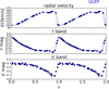 |
Fig. 1 Light and radial velocity curves for U Lep. Plots corresponding to all stars from our sample are available on Zenodo. |
4 Determinations of p-factors and mean radii for nine RR Lyrae stars
We did not notice any apparent discrepancies between courses of radial velocity and light curves. Thus, we did not apply any phase cuts aimed at the exclusion of the potential shocks in the stellar atmosphere where SBCRs would be significantly different than for other pulsation phases. Also, we did not perform any kind of optimization of the scatter of our fits of p-factors based on phase shifts between different observed curves.
Figure 2 presents variations of an integral of stellar radial velocities and angular diameters, while Fig. 3 shows a fit of linear bisector to relation between the integrals and angular diameters for an exemplary star from our sample. The collection of plots for all stars is available on Zenodo. Table 2 presents values of obtained p-factors and Table 3 presents derived mean radii depending on a given SBCR.
Error components of fitted parameters associated with statistical uncertainties of observables (photometric magnitudes, radial velocities, and parallaxes) were estimated using Monte Carlo simulations based on the random variations of values corresponding to individual datapoints within their statistical uncertainties. In the case of the photometry, we assumed values of statistical uncertainties to be 0.01 mag. They correspond to the typically observed scatter on our light curves, and the output from DAOPHOT yields uncertainties of the aperture photometry of the order of 2 mmag. Figure 4 presents an example of distributions of possible p-factors resulting from the propagation of statistical uncertainties of observables for the four considered SBCRs. Figure 5 presents analogous distributions of the possible mean radius values.
In the case of the p-factor, the influence of systematic errors of photometry on the determination is small, with the approximate change in p of 0.025 mag−1 for the V band and 0.085 mag−1 for K (we may see it on Fig. 6). For the mean stellar radii, the corresponding errors associated with systematic shifts of light curves are approximately 0.1 R⊙ mag−1 and 0.35 R⊙ mag−1 for V and K, respectively (Fig. 7). We repeated the procedure of the estimation of this component of uncertainty for each star individually. The accuracy of the V photometry, tied up to the Gaia catalog is similar to that of the K-band photometry with its zero point based on the 2MASS catalog. In both cases, we assumed the possible 1σ systematic shift of a light curve of 0.02 mag.
The influence of the reddening estimation errors is relatively small for the IRSB technique, as already mentioned in Sect. 2. Based on Eq. (10), we estimate the components of statistical uncertainties of p and ⟨R⟩. In order to quantify any possible reddening errors, we recalculated E(B − V) values using 3D dust maps of the Milky Way by Green et al. (2019) based on Pan-STARRS1 and 2MASS photometry and Gaia DR2 parallaxes. Table 1 presents E(B − V)G values from Green et al. (2019) for six stars from our sample in the last column. We conservatively assumed the absolute value of the difference between E(B − V)G and E(B − V) applied in the process of dereddening of our photometry as the 1σ uncertainty of E(B − V). For the three stars that were outiside of the Green et al. (2019) maps, we assumed E(B − V) uncertainties of 0.02 mag.
Finally, the total statistical errors of the derived p-factors and radii were obtained by the quadratic addition of errors resulting from the statistical uncertainties of observables, uncertainties associated with the accuracy of the light curve zero points, and uncertainties of the reddening estimation. Using an example of U Lep and the SBCR of Kervella et al. (2004a), we may divide the statistical uncertainty σp of the determination of its p-factor and the statistical uncertainty, σR, of the determination of its mean radius into the following components associated with uncertainties of different quantities:
parallax: σp,ϖ = 0.022, σR,ϖ = 0.093 R⊙,
radial velocity: σp,RV = 0.015, σp,RV = 0.0003 R⊙,
V- magnitude (stat.): σp,V = 0.009, σp,V = 0.0018 R⊙,
K- magnitude (stat.): σp,K = 0.026, σp,K = 0.0053 R⊙,
V- mag zero point: σp,zpV = 0.005, σp,zpV = 0.019 R⊙,
K- mag zero point: σp,zpK = 0.017, σp,zpK = 0.069R⊙,
E(B − V) reddening: σp,E(B–V) = 0.009, σp,E(B–V) = 0.035 R⊙.
in total, σp = 0.042 and σR = 0.12 R⊙ in that case. We may see that the biggest components of the uncertainty of the p-factor are associated with the precision of the K-band photometry and the uncertainty of the parallax. The smallest components of σp result from the finite accuracy and precision of the V-band photometry and the uncertainty of the reddening. The biggest factors contributing to the error of the mean radius are the uncertainties on the parallax and the accuracy of the K-band photometry, while the contribution of the precision of radial velocities and photometry is virtually negligible.
We obtained mean values of p-factors of stars from our sample of 1.44, 1.40, 1.39, 1.45, and the corresponding root mean square (rms) scatters of their values of 0.076, 0.078, 0.068, and 0.076 for SBCRs reported by Kervella et al. (2004a), Kervella et al. (2004b), Graczyk et al. (2021), and Salsi et al. (2021), respectively. We derived a relation between the p-factor and log P for RRab stars based on the SBCR of Graczyk et al. (2021), which yields the lowest scatter of p-factor values among all considered SBCRs:
![Mathematical equation: $\[\log (p)_G=(-1.06 \pm 0.47) \times[\log (P)+0.25]+1.398 \pm 0.022.\]$](/articles/aa/full_html/2024/10/aa49850-24/aa49850-24-eq14.png) (11)
(11)
While the SBCR of Graczyk et al. (2021) yields, on average, the lowest value of the p-factor, the zero point of p-factors based on Salsi et al. (2021) is the largest:
![Mathematical equation: $\[\log (p)_s=(-1.17 \pm 0.46) \times[\log (P)+0.25]+1.453 \pm 0.022.\]$](/articles/aa/full_html/2024/10/aa49850-24/aa49850-24-eq15.png) (12)
(12)
We notice that relatively large uncertainties of slopes do not allow for any unequivocal statement to be made about the correlation between period and the p-factor. The relation is mostly constrained by two stars (Fig. 8).
Compared to the previous study of Bras et al. (2024), we obtain values of p-factors that are systematically larger using the IRSB technique. The authors report the mean p-factor value for their sample of 17 stars of p = 1.248 ± 0.022 − this is 0.14–0.20 smaller than mean values of p-factors obtained in this work, depending on the SBCR. We have one star in common with the sample from Bras et al. (2024). It is RX Eri for which Bras et al. (2024) report pB = 1.25 ± 0.02. In our case, depending on the SBCR, we obtain values between p = 1.438 ± 0.039 and p = 1.492 ± 0.042. Again, we note that the two implementations of the BW method are different and they are more sensitive to different components of the p-factor. It confirms that p depends on the implementation of the BW method for RR Lyrae stars. Bras et al. (2024) report the rms scatter of p-factor values of 0.09. This is coherent with values obtained in our analysis (0.07–0.08).
The SBCRs for dwarfs and subgiants yield very similar values of mean radii (especially based on the most recent works of Graczyk et al. 2021 and Salsi et al. 2021; see Table 3 and Fig. 7) and the SBCR of Kervella et al. (2004b), which is the only considered relation calibrated for classical Cepheids, gives slightly larger radii. All obtained values are still in good agreement given their uncertainties. The SBCR of Graczyk et al. (2021) gives the following PR relation:
![Mathematical equation: $\[\log \left(\frac{\langle R\rangle}{R_{\odot}}\right)_G=(0.75 \pm 0.11) \times[\log (P)+0.25]+0.7148 \pm 0.0051.\]$](/articles/aa/full_html/2024/10/aa49850-24/aa49850-24-eq16.png) (13)
(13)
The period pivot value of log(P0) = −0.25 was used in order to minimize uncertainties of fitted intercepts and minimize the correlation between the coefficients of the intercept and the slope. In the case of the Kervella et al. (2004b) SBCR for classical Cepheids, the relation is as follows:
![Mathematical equation: $\[\log \left(\frac{\langle R\rangle}{R_{\odot}}\right)_K=(0.73 \pm 0.12) \times[\log (P)+0.25]+0.7268 \pm 0.0057.\]$](/articles/aa/full_html/2024/10/aa49850-24/aa49850-24-eq17.png) (14)
(14)
Both results are in a very good agreement3 with a theoretical prediction for RRab stars by models of Marconi et al. (2005):
![Mathematical equation: $\[\log \left(\frac{\langle R\rangle}{R_{\odot}}\right)_{M 2005}=(0.65 \pm 0.03) \times \log (P)+0.90 \pm 0.03.\]$](/articles/aa/full_html/2024/10/aa49850-24/aa49850-24-eq18.png) (15)
(15)
In a more recent work, Marconi et al. (2015) derived a well-constrained PR relation based on the modeling, as follows:
![Mathematical equation: $\[\log \left(\frac{\langle R\rangle}{R_{\odot}}\right)_{M 2015}=(0.55 \pm 0.02) \times \log (P)+0.866 \pm 0.003.\]$](/articles/aa/full_html/2024/10/aa49850-24/aa49850-24-eq19.png) (16)
(16)
The zero points of the PR relations derived in this work are in good agreement and the slopes are still in 2σ agreement with the above relation.
Bras et al. (2024) found the PR relation for RRab stars in the following form:
![Mathematical equation: $\[\log \left(\frac{\langle R\rangle}{R_{\odot}}\right)_{B 2024}=(0.770 \pm 0.003) \times \log (P)+0.9189 \pm 0.0002.\]$](/articles/aa/full_html/2024/10/aa49850-24/aa49850-24-eq20.png) (17)
(17)
We may see that both the slopes and the intercepts of PR relations derived in this work are in a remarkable agreement with the corresponding relation from Bras et al. (2024). For the single star common for the two samples, RX Eri, Bras et al. (2024) obtained the mean radius of ⟨R⟩B = (5.54 ± 0.18)R⊙, while our IRSB analysis yields the values between (5.40 ± 0.11)R⊙ and (5.55 ± 0.11)R⊙, which again shows a good compatibility between the two different implementations of the BW method for the purpose of the radius determination. Figure 9 presents the two fitted relations between mean radii and pulsation periods of RRab stars.
Different p-factor values obtained using different SBCRs.
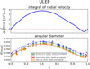 |
Fig. 2 Value of the integral of the radial velocity curve and variations of the stellar angular diameter obtained based on the four SBCRs described in the text. Plots corresponding to all stars from our sample are available on Zenodo. |
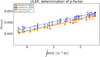 |
Fig. 3 Fits of linear bisectors to relations between values of the integral and the angular diameter estimated based on the four SBCRs. Slope of such a line is a product of the p-factor and the stellar parallax. Plots corresponding to all stars from our sample are available on Zenodo. |
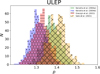 |
Fig. 4 Distributions of probable values of p-factors for U Lep resulting from the Monte Carlo simulations obtained for the four SBCRs. |
Mean radii of stars from our sample obtained using different SBCRs.
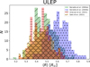 |
Fig. 5 Distributions of probable values of mean radius of U Lep resulting from the Monte Carlo simulations obtained for the four SBCRs. |
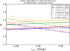 |
Fig. 6 Dependence of the p-factor on the systematic shifts of V- and K-band light curves for different SBCRs in the case of U Lep. |
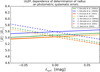 |
Fig. 7 Dependence of the mean radius on the systematic shifts of V- and K-band light curves for different SBCRs in the case of U Lep. |
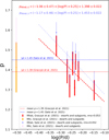 |
Fig. 8 Relations between the p-factor and the pulsation period for RRab stars based on the SBCRs of Graczyk et al. (2021) and Salsi et al. (2021). The rms scatters around relations for RRab stars are reported at the bottom. |
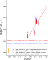 |
Fig. 9 Relations between the radius and the pulsation period for RRab stars based on the SBCRs of Graczyk et al. (2021) and Kervella et al. (2004b). The rms scatters around relations for RRab stars are reported at the bottom. |
5 Discussion and summary
As stressed in the original paper devoted to the Gaia synthetic photometry (Gaia Collaboration 2023), the Johnson-Kron-Cousins photometry has been standardized using the Landolt collection and validated using the Stetson collection (references therein). As can be seen in their Fig. 3, the authors recreate V-band magnitudes of stars with the scatter of about 0.02 mag. It is the same value that has been applied by us as the expected value of the systematic shift for the V-band light curves in our error estimation.
In parallel, we performed a test of the zero point of our K-band photometry tied to the 2MASS system by calculating average magnitudes from our light curves and comparing them with the catalog (single-epoch) values (Cutri et al. 2003). The mean value of the difference between our average magnitude and the catalog values is 0.005 mag and the median value is −0.0003 mag. It indicates that our K-band photometry is indeed well tied to the 2MASS catalog. However, as the typical magnitude error of a single comparison star in the 2MASS catalog is also about 0.02 mag, we applied this value in the estimations of error components of p-factors and mean radii corresponding to photometric zero points of our light curves.
We present results based on four different SBCRs. For two of them (Kervella et al. 2004a; Graczyk et al. 2021), the validity domain corresponds to (V − K) colors of stars from our sample; whereas the SBCRs of Kervella et al. (2004b) and Salsi et al. (2021) were calibrated for slightly different color spans. The SBCR of Kervella et al. (2004b) is also the only considered in this work that was calibrated for classical Cepheids, with others being calibrated for dwarfs and subgiants. Still, when we look at results of the determination of the p-factor for the object U Lep that has extremely low color in our sample with (V − K) between 0.41 and 1.39, we see that the p-factor obtained from SBCR for classical Cepheids (Kervella et al. 2004b) is nearer to the value reported in Graczyk et al. (2021) than what we get from the other two relations devoted to dwarfs and subgiants. Generally, p-factors resulting from the relation from Kervella et al. (2004b) are very similar to those based on Graczyk et al. (2021). The SBCR of Salsi et al. (2021) yields maximum p-factor values among all considered SBCRs. On the other hand, the relation from Graczyk et al. (2021) gives the lowest values of p. The SBCR of Graczyk et al. (2021) yields the lowest scatter of p-factor values (0.068), while p obtained based on Kervella et al. (2004b) have the biggest observed scatter (0.078). Values of obtained p-factors can be interpreted as ratios of amplitudes of angular diameter curves and integrated radial velocity curves. It is also associated with the slope of the relation between the angular diameter and the value of the integral (Eq. (5)). Relative changes, namely, the course of the angular diameter curve (and not its zero point) is crucial for the determination of p. On the other hand, the mean diameter depends on both the zero point of the angular diameter and the p-factor (Eq. (6)). Here, the three SBCRs for dwarfs and subgiants yield similar ⟨R⟩ (with the relations from Graczyk et al. 2021 and Salsi et al. 2021 giving virtually the same values) and radii based on the relation for classical Cepheids are slightly larger.
Nardetto et al. (2023) studied the influence of SBCR’s slope and zero point on the value of p-factor for the case of the classical Cepheid η Aql. They found that the choice of SBCR can influence the value of p at the level of 8%. The authors also found that the method of determination of radial velocities is crucial for the absolute value of p at the level of 9%. The increase of E(B − V) color excess by 0.1 mag would decrease the value of p by about 3%. A possible effect of visual magnitude excess of 0.1 mag would correspond to only 1.5% of bias in the determination of the p-factor, while in the case of the same excess in the K band, the bias would increase to around 6%.
Generally, in the case of the determination of p-factors, the influence of the uncertainty of the zero point of photometry is of the order of the magnitude smaller than the uncertainty component resulting from the combined influence of the parallax, magnitude, and radial velocity statistical uncertainties. Parallax uncertainty propagation plays a crucial role in determining the uncertainties of mean radii. As (V − K) color-based SBCRs are almost parallel to the reddening vector, the reddening uncertainty has virtually negligible contribution to total uncertainties of p-factors. It plays a bigger (but not dominant) role in the estimations of mean radii errors.
Bras et al. (2024) obtained p-factors of 17 Galactic RR Lyrae stars (all of them being fundamental pulsators). The approach presented in that work differs from the IRSB technique, namely: instead of using SBCR, the authors rely on the analysis based on atmosphere models and measurements of many different observables (i.e., photometry in different bands that probe the stellar spectrum in given intervals and radial velocities). The analysis presented there was performed using the SPIPS modeling tool (Mérand et al. 2015). The values of p-factors presented in the work of Bras et al. (2024) are systematically smaller than those derived using the IRSB technique with the mean p-factor value of Bras et al. (2024) being smaller by 0.14–0.20 (depending on the SBCR used in the analysis). However, we obtained very similar scatter of the p-factor values of around 0.07–0.08, whereas Bras et al. (2024) reported a value of 0.09 for their sample. In our case, the scatter for fundamental pulsators drops to 0.05 after the linear detrending, namely, through the calculation of the rms of residuals of the linear fit to the Pp relation. However, our linear Pp relation is not well constrained and the uncertainties on its parameters are significant. The observed discrepancy in p-factor determinations yet again hints at the fact that values of p are dependent on the applied technique. Our determinations of mean radii of RR Lyrae stars are in good correspondence with both the theoretical predictions by Marconi et al. (2005, 2015) and results from the analysis performed by Bras et al. (2024) based on the SPIPS tool.
The future extension of our sample of RR Lyrae stars from the solar neighborhood will allow us to better constrain the parameters of Pp and PR relations for RR Lyrae stars resulting from the IRSB analysis. We note that all applications of the BW method are demanding, especially in terms of the observing time needed for dense coverage of the light and radial velocity curves.
Data availability
Tables containing radial velocity and photometric measurements gathered for the purpose of this work are available at the CDS via anonymous ftp to cdsarc.cds.unistra.fr (130.79.128.5) or online https://cdsarc.cds.unistra.fr/viz-bin/cat/J/A+A/690/A295.
The collection of plots corresponding to all stars from our sample is available on Zenodo under the following link: https://zenodo.org/records/13381583.
Acknowledgements
We thank the anonymous referee for their constructive and valuable comments that contributed to the final form of this article. The research leading to these results has received funding from the European Research Council (ERC) under the European Union’s Horizon 2020 research and innovation program (grant agreement No. 951549). The research was possible thanks to the Polish Ministry of Science and Higher Education grant 2024/WK/02. W.G. gratefully acknowledges support from the ANID BASAL project ACE210002. The research was based on data collected under the ESO/CAMK PAN – OCM agreement at the ESO Paranal Observatory and Polish-French Marie Skłodowska-Curie and Pierre Curie Science Prize awarded by the Foundation for Polish Science. N.N. acknowledges the support of the French Agence Nationale de la Recherche (ANR), under grant ANR-23-CE31-0009-01 (Unlockpfactor). Supported by the National Science Center, Poland, Sonata BIS project 2018/30/E/ST9/00598. Based on observations collected at the European Organisation for Astronomical Research in the Southern Hemisphere under ESO programmes CN2016B-150, CN2017A-121, CN2018A-40, CN2019B-64, CN2020B-42, CN2020B-69, 099.D-0380(A), 0100.D-0339(B), 0100.D-0273(A), 0102.D-0281(A), 0105.20L8.001, 0105.20L8.002, P105.A-9005(A), 105.2045.001, 105.2045.002, 0106.D-0676(B), 0106.D-0691(A, B, C), 106.21T1.001, 108.D-0636(A, B), 108.D-0624(A). This research has made use of the International Variable Star Index (VSX) database, operated at AAVSO, Cambridge, Massachusetts, USA.
References
- Akima, H. 1970, J. ACM, 17, 589 [Google Scholar]
- Astropy Collaboration (Robitaille, T. P., et al.) 2013, A&A, 558, A33 [NASA ADS] [CrossRef] [EDP Sciences] [Google Scholar]
- Baade, W. 1926, Astron. Nachr., 228, 359 [NASA ADS] [CrossRef] [Google Scholar]
- Barnes, T. G., & Evans, D. S. 1976, MNRAS, 174, 489 [Google Scholar]
- Bertin, E. 2006, ASPC, 351, 112 [NASA ADS] [Google Scholar]
- Bertin, E., & Arnouts, S. 1996, A&AS, 117, 393 [NASA ADS] [CrossRef] [EDP Sciences] [Google Scholar]
- Blackwell, D. E., & Shallis, M. J. 1977, MNRAS, 180, 177 [NASA ADS] [CrossRef] [Google Scholar]
- Blažko, S. 1907, AN, 175, 325 [Google Scholar]
- Brahm, R., Jordán, A., & Espinoza, N. 2017, PASP, 129, 4002 [Google Scholar]
- Bras, G., Kervella, P., Trahin, B., et al. 2024, A&A, 684, A126 [NASA ADS] [CrossRef] [EDP Sciences] [Google Scholar]
- Cacciari, C., Clementini, G., Prevot, L., & Buser, R. 1989a, A&A, 209, 141 [NASA ADS] [Google Scholar]
- Cacciari, C., Clementini, G., & Buser, R. 1989b, A&A, 209, 154 [NASA ADS] [Google Scholar]
- Cardelli, J. A., Clayton, G., C., & Mathis, J. S. 1989, ApJ, 345, 245 [CrossRef] [Google Scholar]
- Carney, B. W., & Latham, D. W. 1984, ApJ, 278, 241 [NASA ADS] [CrossRef] [Google Scholar]
- Carney, B. W., Storm, J., & Jones, R. V. 1992, ApJ, 386, 663 [CrossRef] [Google Scholar]
- Castelli F., & Kurucz R. L. 2003, New Grids of ATLAS9 Model Atmospheres, eds. N. Piskunov, W. W. Weiss, & D. F. Gray, IAU Symp., 210, 20 [NASA ADS] [Google Scholar]
- Catelan, M., & Smith, H. A. 2015, Pulsating Stars (Wiley-VCH) [CrossRef] [Google Scholar]
- Clementini, G., Cacciari, C., & Lindgren, H. 1990, A&AS, 85, 865 [NASA ADS] [Google Scholar]
- Crestani, J., Braga, V. F., Fabrizio, M., et al. 2021, ApJ, 914, 10 [NASA ADS] [CrossRef] [Google Scholar]
- Cutri, R. M, Skrutskie, M. F., van Dyk, S. et al. 2003, The IRSA 2MASS All-Sky Point Source Catalog, NASA/IPAC Infrared Science Archive [Google Scholar]
- Dekker, H., D’Odorico, S., Kaufer, A., et al. 2000, SPIE, 4008, 534 [NASA ADS] [Google Scholar]
- Di Benedetto, G. P. 2005, MNRAS, 357, 174 [NASA ADS] [CrossRef] [Google Scholar]
- Drimmel, R., & Spergel, D. N. 2001, ApJ, 556, 181 [Google Scholar]
- Fernley, J. A., Lynas-Gray, A. E., Skillen, I. et al. 1989, MNRAS, 236, 447 [NASA ADS] [CrossRef] [Google Scholar]
- Fernley, J. A., Skillen, I., Jameson, R. F., & Longmore, A. J. 1990a, MNRAS, 242, 685 [CrossRef] [Google Scholar]
- Fernley, J. A., Skillen, I., Jameson, R. F., et al. 1990b, MNRAS, 247, 287 [NASA ADS] [Google Scholar]
- Fouqué, P., & Gieren, W. P. 1997, A&A, 320, 799 [Google Scholar]
- Freedman, W. 2021, ApJ, 919, 16 [NASA ADS] [CrossRef] [Google Scholar]
- Gaia Collaboration (Brown, A. G. A., et al.) 2021, A&A, 649, A1 [NASA ADS] [CrossRef] [EDP Sciences] [Google Scholar]
- Gaia Collaboration (Montegriffo, P., et al.) 2023, A&A, 674, A33 [CrossRef] [EDP Sciences] [Google Scholar]
- Gieren, W., Fouqué, P., & Gómez, M. 1997, ApJ, 488, 74 [NASA ADS] [CrossRef] [Google Scholar]
- Gieren, W., Fouqué, P., & Gómez, M. 1998, ApJ, 496, 17 [NASA ADS] [CrossRef] [Google Scholar]
- Gieren, W., Storm, J., Nardetto, N., et al. 2013, IAU Symp., 289, 138 [NASA ADS] [Google Scholar]
- Gieren, W., Storm, J., Konorski, P., et al. 2018, A&A, 620, A99 [NASA ADS] [CrossRef] [EDP Sciences] [Google Scholar]
- Graczyk, D., Pietrzyński, G., Galan, C. et al. 2021, A&A, 649, A109 [NASA ADS] [CrossRef] [EDP Sciences] [Google Scholar]
- Green, G. M., Schlafly, E., Zucker, C., et al. 2019, ApJ, 887, 93 [Google Scholar]
- Hill, S. J. 1972, ApJ, 178, 793 [Google Scholar]
- Hodapp, K. W., Chini, R., Reipurth, B., et al. 2010, SPIE, 7735, 1 [Google Scholar]
- Isobe, T., Feigelson, E.D., Akritas, M.G., & Babu, G.J. 1990, ApJ, 364, 104 [NASA ADS] [CrossRef] [Google Scholar]
- Jacyszyn-Dobrzeniecka, A. M., Skowron, D. M., Mróz, P., et al. 2017, AcA, 67, 1 [NASA ADS] [Google Scholar]
- Jones, R. V. 1988, ApJ, 326, 305 [NASA ADS] [CrossRef] [Google Scholar]
- Jones, R. V., Carney, B. W., Latham, D. W., & Kurucz, R. L. 1987a, ApJ, 312, 254 [NASA ADS] [CrossRef] [Google Scholar]
- Jones, R. V., Carney, B. W., Latham, D. W., & Kurucz, R. L. 1987b, ApJ, 314, 605 [CrossRef] [Google Scholar]
- Jones, R. V., Carney, B. W., & Latham, D. W. 1988a, ApJ, 326, 312 [NASA ADS] [CrossRef] [Google Scholar]
- Jones, R. V., Carney, B. W., & Latham, D. W. 1988b, ApJ, 332, 206 [CrossRef] [Google Scholar]
- Jones, R. V., Carney, B. W., Storm, J., & Latham, D. W. 1992, ApJ, 386, 646 [NASA ADS] [CrossRef] [Google Scholar]
- Jones, R. V., Carney, B. W., & Fulbright, J. P. 1996, PASP, 108, 877 [NASA ADS] [CrossRef] [Google Scholar]
- Jurcsik, J., & Hajdu, G. 2017b, MNRAS, 470, 617 [NASA ADS] [CrossRef] [Google Scholar]
- Jurcsik, J., Hajdu, G., Szeidl, B., et al. 2012, MNRAS, 419, 2173 [NASA ADS] [CrossRef] [Google Scholar]
- Jurcsik, J., Smitola, P., Hajdu, G., et al. 2017, MNRAS, 468, 1317 [NASA ADS] [CrossRef] [Google Scholar]
- Jurcsik, J., Hajdu, G., Dékány, I., et al. 2018, MNRAS, 475, 4208 [Google Scholar]
- Kaufer, A., Stahl, O., Tubbesing, S. 1999, The Messenger, 95, 8 [Google Scholar]
- Karczmarek, P., Pietrzyński, G., Gieren, W., et al. 2015, AJ, 150, 90 [NASA ADS] [CrossRef] [Google Scholar]
- Karczmarek, P., Pietrzyński, G., Górski, M., et al. 2017, AJ, 154, 263 [NASA ADS] [CrossRef] [Google Scholar]
- Kervella, P., Thévenin, F., Di Folco, E., & Ségransan, D. 2004a, A&A, 426, 297 [NASA ADS] [CrossRef] [EDP Sciences] [Google Scholar]
- Kervella, P., Bersier, D., Mourard, D., et al. 2004b, A&A, 428, 587 [NASA ADS] [CrossRef] [EDP Sciences] [Google Scholar]
- Koen, C., Marang, F., Kilkenny, D., & Jacobs, C. 2007, MNRAS, 380, 1433 [NASA ADS] [CrossRef] [Google Scholar]
- Lindegren, L., Bastian, U., Biermann, M., et al. 2021, A&A, 649, A4 [EDP Sciences] [Google Scholar]
- Liu, T., & Janes, K. A. 1990a, ApJ, 354, 273 [NASA ADS] [CrossRef] [Google Scholar]
- Liu, T., & Janes, K. A. 1990b, ApJ, 360, 561 [CrossRef] [Google Scholar]
- Manduca, A., & Bell, R. A. 1981, ApJ, 250, 306 [NASA ADS] [CrossRef] [Google Scholar]
- Marconi, M., Nordgren, T., Bono, G., et al. 2005, ApJ, 623, 133 [Google Scholar]
- Marconi, M., Coppola, G., Bono, G., et al. 2015, ApJ, 808, 50 [Google Scholar]
- Mayor, M., Pepe, F., Queloz, D., et al. 2003, The Messenger, 114, 20 [NASA ADS] [Google Scholar]
- Mérand, A., Kervella, P., Breitfelder, J., et al. 2015, A&A, 584, A80 [NASA ADS] [CrossRef] [EDP Sciences] [Google Scholar]
- Nardetto, N., Fokin, A., Mourard, D., et al. 2004, A&A, 428, 131 [CrossRef] [EDP Sciences] [Google Scholar]
- Nardetto, N., Mourard, D., Mathias, Ph. et al. 2007, ApJ, 471, 661 [Google Scholar]
- Nardetto, N., Gieren, W., Storm, J., et al. 2023, A&A, 671, A14 [NASA ADS] [CrossRef] [EDP Sciences] [Google Scholar]
- Pietrzyński, G., Gieren, W., Szewczyk, O., et al. 2008, AJ, 135, 1993 [Google Scholar]
- Pietrzyński, G., Graczyk, D., Gallenne, A., et al. 2019, Nature, 567, 200 [Google Scholar]
- Pilecki B., Konorski, P., & Górski, M. 2012, IAUS, 282, 301 [NASA ADS] [Google Scholar]
- Queloz, D., Mayor, M., Weber, L., et al. 2000, A&A, 354, 99 [NASA ADS] [Google Scholar]
- Reipurth, B., Chini, R., Lemke, R. 2004, Astron. Nachr., 325, 671 [NASA ADS] [CrossRef] [Google Scholar]
- Rucinski, S., M. 2002, AJ, 124, 1746 [CrossRef] [Google Scholar]
- Salsi, A., Nardetto, N., Mourard, D., et al. 2021, A&A, 652, A26 [NASA ADS] [CrossRef] [EDP Sciences] [Google Scholar]
- Schlafly, E. F., & Finkbeiner, D. P. 2011, ApJ, 737, 103 [Google Scholar]
- Shapley, H. 1918, ApJ, 48, 154 [NASA ADS] [CrossRef] [Google Scholar]
- Skillen, I., Fernley, J. A., Jameson, R. F., et al. 1989, MNRAS, 241, 281 [NASA ADS] [CrossRef] [Google Scholar]
- Skillen, I., Fernley, J. A., Stobie, R. S., Jameson, R. F. 1993, MNRAS, 265, 301 [NASA ADS] [CrossRef] [Google Scholar]
- Skrutskie M. F., Cutri R. M., Stiening R., et al. 2006, AJ, 131, 1163 [NASA ADS] [CrossRef] [Google Scholar]
- Stetson, P. B. 1987, PASP, 99, 191 [Google Scholar]
- Storm, J., Carney, B. W., Latham, D. W. 1994a, A&A, 290, 443 [NASA ADS] [Google Scholar]
- Storm, J., Nordstrom, B., Carney, B. W., Anderson, J. 1994b, A&A, 291, 121 [NASA ADS] [Google Scholar]
- Storm, J., Carney, B. W., Gieren, W., et al. 2004, A&A, 415, 531 [NASA ADS] [CrossRef] [EDP Sciences] [Google Scholar]
- Storm, J., Gieren, W., Fouqué, P., et al. 2011, A&A, 534, A94 [CrossRef] [EDP Sciences] [Google Scholar]
- Szewczyk, O., Pietrzyński, G., Gieren, W., et al. 2008, AJ, 136, 272 [NASA ADS] [CrossRef] [Google Scholar]
- Szewczyk, O., Pietrzyński, G., Gieren, W., et al. 2009, AJ, 138, 1661 [NASA ADS] [CrossRef] [Google Scholar]
- Thompson, I. B., Kałużny, J., Pych, W., et al. 2001, AJ, 121, 3089 [NASA ADS] [CrossRef] [Google Scholar]
- Tody, D. 1986, SPIE, 627, 733 [Google Scholar]
- Trahin, B., Breuval, L., Kervella, P., et al. 2021, A&A, 656, A102 [NASA ADS] [CrossRef] [EDP Sciences] [Google Scholar]
- Wesselink, A. J. 1946, Bull. Astron. Inst. Netherlands, 10, 91 [Google Scholar]
- Welch, D. L. 1994, AJ, 108, 1421 [NASA ADS] [CrossRef] [Google Scholar]
- Virtanen, P., Gommers, R., Oliphant, T. E., et al. 2020, NatMe, 17, 261 [NASA ADS] [Google Scholar]
- Watermann, R. 2012, PhD Thesis, Ruhr-University Bochum, Germany [Google Scholar]
- Wesselink, A. J. 1969, MNRAS, 144, 297 [NASA ADS] [CrossRef] [Google Scholar]
- Zgirski, B. 2022, PhD Thesis, Nicolaus Copernicus Astronomical Center of the Polish Academy of Sciences Warszawa, Poland http://users.camk.edu.pl/bzgirski/phd_thesis_zgirski.pdf [Google Scholar]
- Zgirski, B., Pietrzyński, G., Górski, M., et al. 2023, ApJ, 951, 114 [NASA ADS] [CrossRef] [Google Scholar]
The mean difference between E(B − V) estimations from two different sources for RR Lyrae stars from our sample is 0.018 mag (Table 1). We further estimate the influence of the reddening uncertainty on the derived parameters for each star independently.
Numerical values of measured magnitudes presented in this work correspond to apparent magnitudes and were not dereddened.
We note that putting pivot log(P0) = 0 in, e.g., Eq. (13) would result in the relation’s intercept of 0.902 ± 0.033
All Tables
All Figures
|
Fig. 1 Light and radial velocity curves for U Lep. Plots corresponding to all stars from our sample are available on Zenodo. |
| In the text | |
|
Fig. 2 Value of the integral of the radial velocity curve and variations of the stellar angular diameter obtained based on the four SBCRs described in the text. Plots corresponding to all stars from our sample are available on Zenodo. |
| In the text | |
|
Fig. 3 Fits of linear bisectors to relations between values of the integral and the angular diameter estimated based on the four SBCRs. Slope of such a line is a product of the p-factor and the stellar parallax. Plots corresponding to all stars from our sample are available on Zenodo. |
| In the text | |
|
Fig. 4 Distributions of probable values of p-factors for U Lep resulting from the Monte Carlo simulations obtained for the four SBCRs. |
| In the text | |
|
Fig. 5 Distributions of probable values of mean radius of U Lep resulting from the Monte Carlo simulations obtained for the four SBCRs. |
| In the text | |
|
Fig. 6 Dependence of the p-factor on the systematic shifts of V- and K-band light curves for different SBCRs in the case of U Lep. |
| In the text | |
|
Fig. 7 Dependence of the mean radius on the systematic shifts of V- and K-band light curves for different SBCRs in the case of U Lep. |
| In the text | |
|
Fig. 8 Relations between the p-factor and the pulsation period for RRab stars based on the SBCRs of Graczyk et al. (2021) and Salsi et al. (2021). The rms scatters around relations for RRab stars are reported at the bottom. |
| In the text | |
|
Fig. 9 Relations between the radius and the pulsation period for RRab stars based on the SBCRs of Graczyk et al. (2021) and Kervella et al. (2004b). The rms scatters around relations for RRab stars are reported at the bottom. |
| In the text | |
Current usage metrics show cumulative count of Article Views (full-text article views including HTML views, PDF and ePub downloads, according to the available data) and Abstracts Views on Vision4Press platform.
Data correspond to usage on the plateform after 2015. The current usage metrics is available 48-96 hours after online publication and is updated daily on week days.
Initial download of the metrics may take a while.