| Issue |
A&A
Volume 687, July 2024
|
|
|---|---|---|
| Article Number | A304 | |
| Number of page(s) | 26 | |
| Section | Planets and planetary systems | |
| DOI | https://doi.org/10.1051/0004-6361/202449236 | |
| Published online | 23 July 2024 | |
Observation of meteors from space with the Mini-EUSO detector on board the International Space Station
1
INAF – Astrophysical Observatory of Turin,
Via Osservatorio 20,
10025
Pino Torinese,
Italy
e-mail: This email address is being protected from spambots. You need JavaScript enabled to view it.
2
Department of Physics – University of Turin,
Via Pietro Giuria 1,
10125
Turin,
Italy
3
INFN – Section of Turin,
Via Pietro Giuria 1,
10125
Turin,
Italy
4
Université Paris Cité, CNRS,
Astroparticule et Cosmologie, 10 Rue Alice Domon et Léonie Duquet,
75013
Paris,
France
5
Faculty of Physics – Lomonosov Moscow State University,
1(2), Leninskie gory,
119991
Moscow,
Russia
6
Skobeltsyn Institute of Nuclear Physics – Lomonosov Moscow State University,
1(2), Leninskie gory,
119991
Moscow,
Russia
7
INFN – Section of Rome Tor Vergata,
Via della Ricerca Scientifica 1,
00133
Rome,
Italy
8
RIKEN,
2-1 Hirosawa Wako,
351-0198
Saitama,
Japan
9
KTH Royal Institute of Technology,
Brinellv ${\bar C_{xy}}(t)$ g ¨ en 8,
114 28
Stockholm,
Sweden
10
Department of Physics, University of Rome Tor Vergata,
Via della Ricerca Scientifica 1,
00133
Rome,
Italy
11
Technical University of Munich,
Arcisstraße 21,
80333
Munich,
Germany
12
S.P. Korolev Rocket and Space Corporation Energia,
Lenin str., 4a Korolev,
141070
Moscow area,
Russia
13
ASI, Italian Space Agency,
Via del Politecnico,
00133
Rome,
Italy
14
Omega, Ecole Polytechnique, CNRS/IN2P3,
Route de Saclay,
91120
Palaiseau,
France
15
Department of Astronomy and Astrophysics, The University of Chicago,
5640 S. Ellis Avenue,
60637
Chicago
IL,
USA
16
INFN – National Laboratories of Frascati,
Via Enrico Fermi 54,
00044
Frascati,
Italy
17
Arpa Piemonte,
via Pio VII, 9,
10135
Turin,
Italy
18
Department of Physics, Konan University,
8 Chome-9-1 Okamoto, Higashinada Ward Kobe,
658-8501
Hyogo,
Japan
19
Department of Physics, Colorado School of Mines,
1523 Illinois Street,
80401
Golden
CO,
USA
20
National Centre for Nuclear Research,
ul. Pasteura 7,
02-093
Warszawa,
Poland
21
Faculty of Physics, University of Warsaw,
Ludwika Pasteura 5,
02-093
Warsaw,
Poland
e-mail: This email address is being protected from spambots. You need JavaScript enabled to view it.
22
Stefan Batory Academy of Applied Sciences,
Stefana Batorego 64C,
96-100
Skierniewice,
Poland
Received:
15
January
2024
Accepted:
14
May
2024
Abstract
Context. Observations of meteors in the Earth’s atmosphere offer a unique tool for determining the flux of meteoroids that are too small to be detected by direct telescopic observations. Although these objects are routinely observed from ground-based facilities, such as meteor and fireball networks, space-based instruments come with notable advantages and have the potential to achieve a broad and uniform exposure.
Aims. In this paper, we describe the first observations of meteor events with Mini-EUSO, a very wide field-of-view telescope launched in August 2019 from the Baikonur cosmodrome and installed on board the Russian Zvezda module of the International Space Station. Mini-EUSO can map the night-time Earth in the near-UV range (290-130 nm) with a field of view equal to 44° × 44° and a spatial resolution of about 4.7 km at an altitude of 100 km from the ground. The detector saves triggered transient phenomena with a sampling frequency of 2.5 µs and 320 µs, as well as a continuous acquisition at 40.96 ms scale that is suitable for meteor observations.
Methods. We designed two dedicated and complementary trigger methods, together with an analysis pipeline able to estimate the main physical parameters of the observed population of meteors, such as the duration, horizontal speed, azimuth, and absolute magnitude. To compute the absolute flux of meteors from Mini-EUSO observations, we implemented a simulation framework able to estimate the detection efficiency as a function of the meteor magnitude and the background illumination conditions.
Results. The instrument detected 24 thousand meteors within the first 40 data-taking sessions from November 2019 to August 2021, for a total observation time of approximately 6 days with a limiting absolute magnitude of +6. Our estimation of the absolute flux density of meteoroids in the range of mass between 10−5 kg to 10−1 kg was found to be comparable to other results available in the literature.
Conclusions. The results of this work prove the potential for space-based observations to increase the statistics of meteor observations achievable with instruments operating on the ground. The slope of the mass distribution of meteoroids sampled with Mini-EUSO suggests a mass index of either s = 2.09 ± 0.02 or s = 2.31 ± 0.03, according to two different methodologies for the computation of the pre-atmospheric mass starting from the luminosity of each event.
Key words: instrumentation: detectors / methods: data analysis / methods: observational / telescopes / meteorites, meteors, meteoroids
© The Authors 2024
 Open Access article, published by EDP Sciences, under the terms of the Creative Commons Attribution License (https://creativecommons.org/licenses/by/4.0), which permits unrestricted use, distribution, and reproduction in any medium, provided the original work is properly cited.
This article is published in open access under the Subscribe to Open model. This email address is being protected from spambots. You need JavaScript enabled to view it. to support open access publication.
1 Introduction
Tons of extraterrestrial material enters the Earth’s atmosphere every day, mostly in the form of interplanetary dust particles (IDPs) in the sub-millimetre range (Brownlee 2001; Bradley 2003). Such small particles, also referred to as micrometeoroids, are typically slowed down at the very top of the atmosphere and survive the transit with little or no ablation. On the other hand, a small fraction of these bodies (meteoroids1) are big enough to pierce through the lower part of the atmosphere at hypersonic speed. The atmospheric friction and the extremely high dynamical pressure trigger the ablation phase and the meteoroid starts to decelerate and lose mass. Reaching a temperature of the order of thousands of K, the generated air plasma and the body itself emit light, both from black-body radiation and emission lines of the electronic transition of elements. This light emission phenomenon is called meteor. The residual portion of the meteoroid that survives the atmospheric ablation and eventually falls on the Earth’s surface is called meteorite. For a general overview on the topic, we refer to Ceplecha et al. (1998); Ryabova et al. (2019); Colonna et al. (2019).
The study of the physical and chemical properties of interplanetary matter is crucial in the advancement of our knowledge about the formation and evolution of the Solar System (e.g. Kruijer et al. 2020 and references therein). The recovery of meteorites allows the analysis of the most primitive rocks in the Solar System, which have undergone little to no melting processes (i.e. chondrites). Even if no meteorite can be collected, observations of meteors provide a unique tool for pinpointing the flux of meteoroids to the Earth (Halliday 2001; Zolensky et al. 2006; Drolshagen et al. 2017). Despite the observational effort in the last century, the quantification of such flux as a function of the meteoroid mass is still a matter of debate. The accurate determination of this flux is also crucial to assess the hazard of meteoroid impacts for spacecraft operations, especially in the long-term perspective (Foschini 1999; Moorhead & Matney 2021). As for the most recent example, the primary mirror of the James Webb Space Telescope experienced 25 micrometeoroid hits between March 2022 and January 2023, one of which inflicted significant uncorrectable damage to the instrument (Rigby et al. 2023).
Meteors are typically observed from ground facilities in the optical wavelength range. In particular, meteor and fireball networks have been implemented worldwide since 1960. At present, they have reached a coverage of a few percent of the total Earth’s surface (Spurný et al. 2017; Colas et al. 2020; Devillepoix et al. 2020). These networks are aimed to maximise the efficiency of meteorite recovery and to precisely compute the pre-atmospheric orbits of the observed population of meteoroids, thus enabling investigations about the link between different meteorite classes and their source regions in the Solar System (Granvik & Brown 2018; Jenniskens et al. 2019; Unsalan et al. 2019). Observations from these networks have also been used to infer the flux to the Earth of meteoroids of mass between 10−6 kg and 102 kg (Halliday et al. 1996; Oberst et al. 1998; Koschny et al. 2017). Nonetheless, an accurate determination of the actual exposure of such networks is not trivial (Koschny & Zender 1998; Vida et al. 2022) and may result in significant biases that affect the computation of the meteoroid absolute flux. Alternatively, the meteoroid flux at different mass ranges can be estimated by ground-based meteorite search in hot deserts (Bland et al. 1996; Gattacceca et al. 2011; Hutzler et al. 2016; Drouard et al. 2019) and polar ice (Evatt et al. 2020; Rojas et al. 2021) via stratospheric in situ collection of IDPs (Warren & Zolensky 1994; Cziczo et al. 2001; Rietmeijer et al. 2016), by measuring the lunar cratering rate and impacts (Werner et al. 2002; Suggs et al. 2014) or by satellite observations of bolides (Brown et al. 2002; Jenniskens et al. 2018), among other methods.
The observation of meteors from space presents significant advantages compared to ground-based experiments. Being less dependent on weather and atmospheric conditions, a space-based detection system has the capability of reaching a high exposure time and offers a uniform coverage in both space and time. In spite of these advantages, meteor and fireball detections from space have not been routinely reported in the past. The main reason for a general lack of detection reports in the last decades is that many satellites are equipped to monitor phenomena occurring over much longer timescales than the few seconds characterising the dynamics of a meteor entering the Earth’s atmosphere. Consequently, in many cases meteor events are not recorded or detected. For a long time, there have been satellites equipped with sensors suited for fireball detection; however, they have generally, but not exclusively, been used for military purposes that do not include the scientific study of meteors. Nevertheless, there are the following two noticeable exceptions. The NASA-JPL Center for NEOs Studies (CNEOS) monitors very bright bolides with space sensors. These data are collected by US Government sensors, in the framework of the Nuclear Test Ban Treaty monitoring satellites (Tagliaferri et al. 1994). Such instruments have a rather high energy threshold (total energy E > 0.073 kT TNT) and they detected 973 events from 1988 to March 2024. CNEOS regularly publishes data about these events, including position, velocity, and computed total energy of each event2. Since 2020, they have also been releasing the measured light curves of detected events. Similarly, in 2019, it was determined that the Geostationary Lightning Mapper (GLM) instruments on GOES3 weather satellites can detect fireballs and bolides (Jenniskens et al. 2018; Smith et al. 2021). Their detections are routinely reported online4 and are thus available to the scientific community. To date, GOES satellites have detected about 5000 events in the range from −25° to −180° longitude and ±55° latitude.
The idea of having an instrument in space devoted to meteor observation has been pursued within the JEM-EUSO programme, originally through the JEM-EUSO project (Adams et al. 2015a) and currently through the Mini-EUSO mission (Bacholle et al. 2021) on board the International Space Station (ISS). The main goal of the JEM-EUSO programme is to observe Extreme Energy Cosmic Rays (EECRs, energy E > 5 × 10¹⁹ eV) from space, through the use of a dedicated telescope with a large field of view (FOV) that is able to detect single photons in the near-UV wavelength interval between 290 nm and 430 nm (Adams et al. 2013). However, it has been computed through simulations that these devices also present sensitivity to meteors with absolute magnitudes5 below +7 (JEM-EUSO) and +5 (Mini-EUSO) with a detection rate of the order of ~ 1 per second and ~2 per minute, respectively (Abdellaoui et al. 2017).
Considering a UV detector covering the interval of wavelengths of JEM-EUSO instruments and assuming a typical V band centred at 550 nm, we can expect (as a first approximation) that the flux in the two bands should be comparable. This is due to the fact that both UV and V bands are dominated by Mg, Fe, and Na emission from the warm component (~4500 K) of the ablation products in the meteor wake that is rich in low excitation lines by metal atoms, mainly including Fe, Mg, Na, and Ca. This prediction appears reasonable, even if we take into account that Na sometimes shows differential ablation and can vary among different meteors. Moreover, the V band can also exhibit some air plasma emission from the first positive band of N2, which can cause some variations in the emitted radiance. This means that the flux observed by Mini-EUSO in the UV range might be comparable to the one observed in the visible range. Furthermore, UV observations of meteors from the ground are challenging (due to atmospheric ozone absorption) and almost unprecedented, with only a few recorded events in this wavelength range (Jenniskens et al. 2002; Carbary et al. 2003; Kasuga et al. 2005). However, this is not the case for space-based observations, which allow for an extinction-free spectral domain.
Since October 2019, Mini-EUSO has been operational on the ISS, thus allowing for an assessment of the real performance of the instrument. In this article, we present and discuss the first results of the systematic observations of meteors in the near-UV made by the Mini-EUSO telescope. Section 2 gives an overview of the mission and Sect. 3 presents the methods developed for the search and analysis of meteor events in Mini-EUSO data. We discuss the analysis of meteor observations during the first 40 data-taking sessions in Sect. 4. In Sect. 5, based on our results, we assess the absolute flux of meteors and compare it with other estimations available in the literature, also discussing the slope of the mass distribution which is related to the mass index of the sampled population of meteoroids. Finally, we give our conclusions in Sect. 6.
2 Mission overview
Mini-EUSO (Multiwavelength Imaging New Instrument for the Extreme Universe Space Observatory, known as ‘UV atmosphere’ in the Russian Space Programme) is a telescope operating in the near-UV range, with a square focal surface corresponding to a field of view of about 44° × 44° implemented through two 25 cm Fresnel lenses. The focal surface of Mini-EUSO (PDM, Photon Detector Module) is made of a matrix of 6 × 6 Multi-Anode Photomultiplier Tubes (MAPMTs), which consists of 8 × 8 pixels each, for a total of 2304 channels. The resulting spatial resolution at ground level is approximately 6.3 km × 6.3 km, corresponding to 4.7 km × 4.7 km at the typical meteor altitude of 100 km, varying slightly according to the altitude of the ISS and the pointing direction of each pixel. Mini-EUSO was launched with the uncrewed Soyuz MS-14 on 22 August 2019. The first observations, from the nadir-facing UV transparent window of the Russian Zvezda module, took place on 7 October 2019. The detector is typically installed twice a month during local night-time on the ISS, for about 12 hours of operations.
The detailed technical specifications of Mini-EUSO are reported in Appendix A. The mission was originally conceived for the development of the study of EECR from space (Casolino et al. 2017), as part of an ongoing effort of the Joint Experiment Missions for Extreme Universe Space Observatory (JEM-EUSO) collaboration. For this reason, the detector is mostly sensitive in the 290–430 nm wavelength range (see Fig. A.2), where most of the fluorescence light from extensive air showers (EASs) initiated by cosmic rays interacting in the atmosphere is emitted, due to the return to the ground state of nitrogen molecules (N2) excited by the ionisation of the charged particle component of EAS. Mini-EUSO performs data acquisition in single-photon counting mode thanks to its singular data acquisition system that handles three temporal resolutions simultaneously. The time step of each temporal resolution is called a gate time unit (GTU). Photon counts are summed in a 2.5 µs data stream (called D1), over which sums of 128 frames are calculated (320 µs, D2). Both D1 and D2 data are saved only if a significant signal is detected by a dedicated trigger algorithm over a 128 GTU buffer. On the other hand, sums of 128 D2 frames (40.96 ms, D3) are stored in a continuous acquisition mode. To preserve a similar dynamic range among all three time resolutions, values of pixel counts in D2 and D3 data are conventionally normalised to counts over the time integration of D1.
So far, within the JEM-EUSO programme, various instruments have been constructed and operated on the ground (EUSO-TA, Abdellaoui et al. 2018), on stratospheric balloons (EUSO-Balloon, Adams et al. 2022; EUSO-SPB1, Abdellaoui et al. 2024; EUSO-SPB2, Adams et al. 2017) and in space (TUS, Klimov et al. 2017), in addition to the future planned K-EUSO (Klimov et al. 2022) and POEMMA (Olinto et al. 2021) missions.
Observations in this frequency range and with this combination of temporal and spatial resolution (2.5 µs and ~6 km) are relatively scarce, therefore systematic observations from space can contribute to study several phenomena that take place on the surface of the Earth or in its atmosphere, either with a terrestrial (e.g. transient luminous events, TLE, airglow, gravity waves, etc., Adams et al. 2015b; Marcelli et al. 2022) or extra-terrestrial origin (e.g. meteors, search for strange quark matter, Adams et al. 2015a). The 2.5 µs resolution of Mini-EUSO is suitable to search for EECRs, as their duration can be typically quantified in an order of 100 µs, or for fast TLEs such as emission of light and very low frequency perturbations due to electromagnetic pulse sources (ELVEs), while the 320 µs resolution is appropriate for slower lightnings, and the 41 ms time resolution is well suited for much slower phenomena such as meteors, bioluminescence, the search for strange quark matter (SQM) and the monitoring space debris, among others. Moreover, anthropogenic emissions such as towns, fishing boats, and ground flashers6 can be studied as well thanks to the multiple time resolutions (Casolino et al. 2023).
An overview of the first observations of Mini-EUSO at the different timescales is reported in Bacholle et al. (2021) while a more detailed discussion of Mini-EUSO performance in D1 mode is summarised in Battisti et al. (2022).
3 Methods
We describe and discuss here the various algorithms developed for the tracking and analysis of meteors recorded in the continuous monitoring of Mini-EUSO D3 data. In our case, this task is particularly challenging because the telescope can observe a wide variety of phenomena that may resemble the light curve of a meteor at similar timescales, such as lightning and light sources on the ground. Therefore, we implemented dedicated trigger schemes devoted to the recognition of a moving source in the FOV of Mini-EUSO that could be related to a meteor event, together with both a classification scheme to filter out non-meteor events and an analysis pipeline able to reconstruct the whole flight of the event. From these results, we were able to compute the main physical parameters of the observed meteors, such as duration, horizontal speed, azimuth, and magnitude. Since Mini-EUSO cannot provide a stereoscopic vision of the event, we are not able to triangulate and, therefore, compute the 3D trajectory of the meteor in the atmosphere. Consequently, we make an assumption about the altitude of the observed meteors and, in the next sections, we discuss its impact on the uncertainty of the deduced physical parameters.
3.1 Meteor trigger algorithms
As a first approach to identify meteors in Mini-EUSO D3 data, we adapted a trigger algorithm that was originally designed for the onboard detection of space debris in future missions of the JEM-EUSO programme. A detailed description of the algorithm and its performance for space debris search can be found in Miyamoto et al. (2019). Even if meteors enter the Earth’s atmosphere at a speed within 11–72 km s−1 and are typically faster than space debris (7–9 km s−1), the apparent speeds of these two classes of events as seen from Mini-EUSO are comparable. This is because of the higher distance at which meteors are expected to be observed (~100 km altitude, i.e. about 300 km of distance from the ISS) compared to the distance expected for space debris (tens of kilometres from the ISS).
The concept of this trigger (referred to as “trigger 1” in the following) is detailed in Appendix B.1 and summarised in Fig. B.1. The algorithm looks for tracks of over-threshold pixels in a time window lasting for at least four consecutive GTUs. This occurrence should represent the case of a moving source, such as a meteor, imaged onto the focal surface of Mini-EUS0. Due to its simple and quickly executable implementation, this algorithm could be employed in the future as an online meteor trigger for the planned missions of the JEM-EUSO programme.
At the same time, we developed an alternative trigger method (trigger 2) specifically dedicated to the offline detection of meteors on Mini-EUSO D3 data (Piotrowski et al. 2022). As similarly discussed for trigger 1 in Appendix B.1, the most difficult task to be performed is the filtering of false positives, due to the complex variability of natural background light mainly caused by moving sources on the ground. To discard such events, this trigger implements various custom-made selection processes based on a quantitative evaluation of parameters such as the light curve shape and the spatial compactness of the event, together with a sophisticated background subtraction method. A detailed description of this algorithm is given in Appendix B.2. Its main steps are as follows: (1) estimation of the background level for each pixel; (2) identification of frames over the background-based threshold for each pixel; (3) filtering of (pixel, frame) pairs that do not have another such pair in a four GTUs vicinity; (4) grouping of (pixel, frame) pairs across space and time into events using a KD-tree; and (5) application of quality cuts on meteor candidates to filter false positives from the event lists.
3.2 Event selection and classification
Based on the output of the two trigger algorithms, we visually inspected the events and catalogued them in the following four classes.
The first class is the meteors (M) class and it encloses events of clear meteor origin that show an evident apparent motion on the PDM within more than 2–3 pixels and that have a Gaussianlike single-pixel light curve, originating from the PSF of the meteor gradually moving in and out of the FOV of each pixel.
The second class is that of meteor candidates (M?) and consists of events that cannot be indisputably classified as meteors, but that show some evidence for it and that can therefore be likely considered of meteor origin. A typical example of an event in this class has a smooth light curve but shows a limited and not clear apparent motion on the PDM. This may be caused by various reasons, for instance, the meteor crossing the border in between two adjacent MAPMTs that corresponds to an inactive region equivalent to the size of one pixel insensitive to incoming light. While we usually consider the M and M? classes together (and indicate them as M), we preserved this distinction on the database to have a qualitative measure of the reliability of the classification of meteor events.
All events that show a significant signal in one or more pixels but that are not meteors are included in the third class, namely the non-meteor events (U) class. For example, this is the case of the signal coming from a bolt of lightning that survived the trigger intensity cut-off and did not trigger more than 64 pixels.
The fourth and final class is the noise events (N) class that consists of false positives for which no significant signal is visible at the time and position as indicated by the trigger algorithm. This is often the case of isolated GTUs that triggered in a few pixels near the leading edge of the light curve of a city entering their FOV. In fact, fixed sources on the ground move in the FOV of Mini-EUSO at an apparent speed, namely, the ISS speed (~7.66 km s−1), along the positive y direction.
An example of a meteor event within the M class is represented in Fig. 1. As a first step, this classification process was applied to the first nine data-taking sessions of Mini-EUSO, using a double-blind approach to highlight potential subjective biases of the observers. In particular, the results of this analysis were used to tune the algorithm of trigger 1, to understand its performance (see Appendix B.1 for details) and to design the analysis algorithm to track the entire flight of the meteor in the FOV of Mini-EUSO, as described in Sect. 3.3.
The application of more advanced methods for an automatic and reliable event trigger and classification is currently under investigation for the data of Mini-EUSO and for future missions of the JEM-EUSO programme. For example, a novel convolu-tional neural network (STACK-CNN) was recently developed for the identification of space debris in Mini-EUSO data, successfully tested against simulations (Montanaro et al. 2022) and subsequently adapted for the detection of meteors (Olivi et al. 2023).
3.3 Meteor tracking and analysis
In order to reconstruct the motion of meteors detected on the focal surface of Mini-EUSO, we designed a tracking algorithm that operates starting from the results of the trigger7. In particular, each entry resulting from both trigger algorithms (Sect. 3.1) is provided with an estimation of the starting GTU (the index of the first GTU t0 within the four over-threshold frames) and the corresponding (x0, y0) position in pixel coordinates. From this information, we defined a tool to objectively evaluate if the light curve of that pixel, and the ones within its first neighbourhood, registered a significant signal and if this is compatible with the expected features of a meteor observed on the Mini-EUSO PDM. We can expect that the single-pixel light curve of a meteor resembles a Gaussian profile. This is because this signal is given by the progressive motion within the FOV of each pixel of the PSF of the meteor, which can be approximated by a 2D Gaussian function with an FWHM of 1.2 px (Bacholle et al. 2021). Therefore, we selected a range of [−10, 30] GTU from t0 and fit over this light curve portion, Cxy(t), a Gaussian function summed to a second-degree polynomial background:
 (1)
(1)
where the first three polynomial terms (B0, B1, B2) parameterise the variation of the background over time, A represents the maximum intensity of the signal of the event on the pixel light curve (occurring at the time T) and sd is the standard deviation of the Gaussian profile and, thus, related to the duration of the signal on that pixel. An example of this processing is shown in Fig. 2a, where the measured D3 counts are reported as black stars and the fitted function Fxy(t) from Eq. (1) is plotted by the red line. The blue line represents the background term of Fxy(t), and the shaded blue band plots its 3σ confidence interval. We then define a series of five conditions that the results of the fit and its parameters have to fulfil to positively evaluate the light curve, Cxy(t), and the pixel, (x0, y0), as part of the meteor track, which are as follows: (1) the fit has reached a successful convergence; (2) the fitted value of the Gaussian height A ± σA is significantly greater than zero at the 3σ confidence level (99.9%, one-sided interval), that is, A − 3σA > 0; (3) the light curve Cxy(t) has at least one GTU that is over the 3σ confidence band of the background term of Fxy(t); (4) the fitted centre T of the Gaussian function is determined to be within the allowed range of [−10, +30] GTU from t0; and (5) the fitted standard deviation sd results in a duration of the signal ∆t = 2 · 3 sd compatible with the motion of a meteor within the pixel of Mini-EUS0. Since the speed of a meteor is confined in the range [11.1, 72.8] km s−1 and given the size of the pixel of 4.7 km at an altitude of 100 km, this results in a range of [2,11] GTU of duration. Considering that we actually observe the horizontal component of the speed and that the apparent speed vector of the meteor is measured in the reference frame of the ISS, whose motion can be approximated as a purely horizontal component in the short time covering the detection event, we allow for a pixel duration of [2, 20] GTU.
If all of these conditions are matched, we consider the corresponding pixel as significant and add it to the list of the meteor track (xi,yi, tik), where tik ∊ [Ti − 3sdi, Ti + 3sdi], i is the pixel index and k is the GTU index. This procedure is repeated iteratively, as presented in Fig. 2b. Once a pixel is added to the track, all its first neighbours are added to the processing list and checked for their significance through the aforementioned conditions. Given the sampling time of 41 ms, the meteor speed of the order of tens of km s−1 and the PSF size on the PDM, we expect the transition between pixels to be relatively slow. As a consequence, for all the pixels (except the first one), we added a sixth condition; namely, we check whether the centre, T, of the Gaussian profile is contained within the duration of one of the other pixels of the track (according to condition 5).
An example of the results of this meteor tracking algorithm is presented in Fig. 3. Panel a shows the map of pixels on the PDM that were recognised as part of the meteor event, and panel b plots their light curves, with the coloured portion highlighting the duration of the event on each of them. The integral light curve of the event is plotted in panel c and it is obtained by summing all the single-pixels light curves. We can then use the polynomial term from Eq. (1) to remove the background contribution to single-pixel light curves:
 (2)
(2)
which is plotted in panel d, and also for the integral light curve of the event in panel e. It has to be noted that, in this case, the apparent trajectory of the meteor on the PDM crossed the border between two MAPMTs. While this is not represented in Fig. 3a, each MAPMT is physically separated from the others, resulting in an inactive region of the width of ~1 px at all of its borders. When the PSF of the meteor on the PDM is projected on these borders, a substantial fraction of its light is lost, as evident from the integral light curve of panels c and e.
The net counts  , namely the signal attributed only to the meteor captured on the PDM, are therefore used to compute the barycentre position of the meteor along its apparent trajectory, which is simply given as:
 (3)
(3)
for the x coordinate and where the sum over i extends over all the identified pixels (xi, yi) of the meteor track. The same formula is valid for the y coordinate as well. To be able to compute the physical parameters of the meteor, we then need to convert the derived pixel positions into physical coordinates, namely the distance from the FOV centre measured in km in the x and y directions. The footprint of each pixel depends on the distance of the meteor from Mini-EUSO, that is d = HISS − H. While the altitude of the ISS orbit HISS is reported in the metadata of the observations, we do not have any evidence to deduce the altitude H of the meteor because Mini-EUSO only implements a monocular vision and cannot triangulate the 3D trajectory of the event. We are then forced to make an assumption about the typical meteor altitude of H0 = 100 km. The effects of this assumption on the accuracy and precision of the physical parameters of the meteor measured by Mini-EUSO are discussed in Sect. 4.4. Even at a fixed altitude, the footprint of each pixel is not homogeneous on the PDM due to optical distortions. Therefore, we use the simulation results of the optical system of Mini-EUSO to account for these secondary effects (Abe et al. 2023). For example, the footprint on the ground (d ≃ 420 km) of Mini-EUSO pixels varies from ~35 km2 at the very centre of the FOV to ~26 km2 at its borders, corresponding to a variable linear dimension from approximately 6 km to 5 km (Bacholle et al. 2021; Casolino et al. 2023).
The resulting barycentre positions for the event presented in Fig. 3 are plotted in Fig. 4. The effect of the MAPMT gap crossing is again evident on panel c, where the computed y position has a sudden variation of ~10 km, namely, a jump of approximately two pixels, when the PSF of the meteor transits between the two MAPMTs, as shown in panel a. We, therefore, compute the Vx and Vy speed components of the meteor by applying a linear fit over these positions (solid lines of panels b and c) and estimate the apparent horizontal speed V and azimuth direction a. For both these quantities, we correct for the apparent speed of the ISS (VISS ≃ 7.66 km s−1) and azimuth of motion, which is also provided in the metadata and, in a first approximation8, is oriented along the positive y direction of the PDM:
 (4)
(4)
 (5)
(5)
Equation (5) represents the arrival direction of the meteor counted clockwise from the north, and aISS is the local azimuth of the ISS orbit. For the event of Fig. 4, we computed a horizontal speed of 53.8 km s−1 and an azimuth angle of 53.9°. The uncertainties affecting these values are discussed in Sect. 4.4.
 |
Fig. 1 Example of a meteor event detected by the Mini-EUSO telescope on board the ISS, imaged on D3 data during session no. 14 on 01/04/2020 at 00:49:17 UT over the South Atlantic Ocean (9°33′ S, 4° 19′ W) and classified as an M event in the Mini-EUSO meteor database (see Sect. 3.2). The event lasted for 32 GTU, from 00:49:16.72 to 00:49:18.03 UT (~1.3 s). At that time, the ISS was moving in orbit at an altitude of about 424 km from the ground at a speed of 7.66 km s−1, with an apparent motion projected on the ground oriented along the SSE direction, at an azimuth of ~144° counted clockwise from the North. (a) Reconstructed track of the meteor on the PDM of Mini-EUSO, obtained by a selective integration of D3 images over the pixels lightened up by the event. The apparent motion of the ISS on the PDM is approximately oriented along the positive y direction. (b–g) Zoom of the PDM in the region x ∊ [14, 24] px–y ∊ [9, 19] px (highlighted in panel a by the red box) for subsequent times every 4 GTU (~0.16 s). On all panels, dashed lines mark the border of adjacent MAPMTs corresponding to a physical separation on the PDM of ~1 px which is not sensitive to incoming light. The presence of these gaps is visible, for example, when the meteor track crosses the border between two MAPMTs around GTU 2477 (panels e–f), at which time the meteor dims because part of the light is focused on this inactive region of the PDM. |
 |
Fig. 2 Schematisation of the tracking algorithm designed to reconstruct the meteor path imaged on the PDM of Mini-EUSO in D3 data. (a) Example of the fit of the Gaussian profile of Eq. (1) to identify the meteor signal. Black stars represent the measured light curve of the pixel, the red line is the fitted Gaussian function and the blue line and shaded band plot the background polynomial term with its 3σ confidence interval. (b) Graphical representation of the iterative process to identify all the pixels within the meteor track. We start from the first pixel provided by the trigger algorithm and evaluate its significance (green square in the first box from the left), then we add to the processing list all of its first neighbours (blue pixels), which are again evaluated by the fitting of panel a. Some of them will be discarded (orange pixels). Every time a new pixel is added to the track, all of its first neighbours are added to the processing list if they had not already been checked, until no more pixels are found to be significant. |
 |
Fig. 3 Results of the meteor tracking algorithm for one event of the Mini-EUSO session no. 11, occurred on 21/02/2020 at 20:05:55.15 UT over the Indian Ocean (20°56′ S, 93°56′ E). (a) Map of the identified pixel within the track on the PDM; (b) measured light curves of all the coloured pixels of panel a plotted with matching colours and highlighting the GTU range corresponding to the transit of the meteor projected on each individual pixel; (c) integral light curve obtained by summing the ones of panel b; (d) light curves of net counts of the meteor obtained according to Eq. (2); (e) integral net light curve. In its apparent motion, the meteor crosses the border between two MAPMTs, as evident from the decreased counts around GTU 1990 on the plots of panels c and e. In these panels, the red curves plot the total light curve derived from the fit results, namely, the Gaussian term of Eq. (1) summed over all the pixels in the track. |
 |
Fig. 4 Results of the barycentre computation for the event presented in Fig. 3. In all panels, the black points and lines represent the results of the computation over the net measured counts |

4 Results and discussion
4.1 The meteor database
We used the two trigger methods described in Sect. 3.1 to process the Mini-EUSO observation dataset from November 2019 up until August 2021, consisting of sessions from no. 05 to no. 44. Table 1 reports the meteor trigger counts and rates of each session for trigger 1 (Appendix B.1) and trigger 2 (Appendix B.2). In general, trigger 2 shows better performances with respect to trigger 1 in terms of the percentage of false positives, which is always confined to <20%. The two triggers show a comparable event rate (given in Table 1 as events per minute) in all the sessions, with a slightly better performance of trigger 2, as expected. With a total observation time of 8200 min (corresponding to 136.7 hours or 5.7 days), trigger 1 detected 14.4 thousand events at an average rate of 1.76 min−1, while trigger 2 detected 18.3 thousand events at 2.23 min−1. However, the comparison between the two datasets highlights that only ~36% of the events are detected by both triggers (column ‘CM’ of Table 1). Of the remaining fraction, 24% of the meteor events are detected only by trigger 1 (Col. ‘T1’), and 40% only by trigger 2 (Col. ‘T2’). While this evidence may look peculiar at first sight, we have to consider that the majority of events seen by Mini-EUSO are quite faint, between magnitudes of +3 and +5 and with a limiting magnitude of the telescope for meteor observations of about +6 in the U band (see Sect. 4.3). As discussed in Sect. 5, the efficiency of trigger 1 for meteors in this magnitude range at a typical background value of 1 cnts GTU−1 is ~50%. Therefore, it is reasonable that two different triggers may detect two sets of events that are only partially overlapping. Furthermore, since trigger 1 detected 60% and trigger 2 detected 76% of the overall number of events, a random intersection of the two subsets will consist of 46% of the total. The observed fraction of 36% of common events is not far from this value; nonetheless, being lower than 46%, it suggests the presence of a selection bias. Indeed, the fraction of common events is higher for bright events (~45% between +1 and +3 absolute magnitude) and closer to the expected value for a random selection of 52% (resulting from 67% of events detected by trigger 1 and 78% detected by trigger 2).
Because of this result, we then consider the merged version of these datasets (‘total’ columns in Table 1) consisting of 24 thousand meteors detected at an average rate of 2.92 min−1. This rate is quite close to the expected value computed for Mini-EUSO observations of meteors at +5 absolute magnitude of 2.4 min−1 (Abdellaoui et al. 2017). Finally, Fig. 5 shows the spatial density distribution of this meteor dataset. About 30% of the total number of meteors is observed over land, while 70% of them are triggered over the oceans. This is in agreement with the ratio of the land- over ocean-covered area on a global scale. Nevertheless, as already highlighted in Sect. 3.2, we can observe that meteors rarely trigger over populated and light-polluted areas such Western and Central Europe, North America, and India, to mention a few. The poorer rate of meteor detection on the Pacific Ocean compared to the Atlantic one is due to the starting time of operation of Mini-EUSO, occurring usually at approximately 18:30 UTC. Consequently, during the 12 hours of operation, the Pacific Ocean is predominantly in the daytime.
4.2 Magnitude system for Mini-EUSO
To convert the intensity of each meteor measured by Mini-EUSO in cnts GTU−1 units to an estimation of its absolute magnitude ℳ, we need to define the zero-point of the magnitude system of Mini-EUSO, namely, the reference flux of a source of absolute magnitude ℳ = 0 observed at an altitude of 100 km from the ground. Figure A.2 plots the photon detection efficiency curve of the telescope, which observes in the near-UV wavelength range, from 260 nm to 480 nm. Among the standard photometric systems, the closest bandpass filter is the Johnson-Cousins U band (Landolt 2009), which has a maximum at λ ≃ 370 nm in close agreement with the one of the Mini-EUSO bandpass (365 nm). However, the U band is a bit narrower and spans approximately from 310 nm to 410 nm of wavelength. Since Mini-EUSO does not observe any standard calibration sources (i.e. stars) in its FOV during regular operations, we rely on the reference flux of the U band to estimate the zero-point flux as:
 (6)
(6)
where ƒλ = 4.175 × 10⁻⁸ erg cm−2 s−1 nm−1 is the zero-point flux of the U band, A = π(12.5 cm)2 = 490.6 cm2 is the photon collecting (lenses) area of the Mini-EUSO telescope, ∆tD1 = 2.5 µs is integration time of D1 data, ∆λ = 220 nm is the width of the Mini-EUSO wavelength bandpass, η ≃ 3.7% is the integral average efficiency of Mini-EUSO over ∆λ and Eγ = 5.45 × 10⁻¹² erg is the nominal energy of a photon at λ = 365 nm. Therefore, the absolute magnitude, ℳ(t), of the meteor is computed according to the following:
![Mathematical equation: $\matrix{ {{\cal M}(t) = - 2.5{{\log }_{10}}\left[ {{{\sum\nolimits_i {{{\bar C}_i}(t)} } \over {{F_0}}}} \right]} \hfill \cr {\,\,\,\,\,\,\,\,\,\,\, - 5{{\log }_{10}}\left[ {{{\sqrt {{x_{\rm{b}}}{{(t)}^2} + {y_{\rm{b}}}{{(t)}^2} + {{\left( {{H_{{\rm{ISS}}}} - {H_0}} \right)}^2}} } \over {100{\rm{km}}}}} \right],} \hfill \cr } $](/articles/aa/full_html/2024/07/aa49236-24/aa49236-24-eq9.png) (7)
(7)
where xb and yb are the barycentre positions from the centre of the FOV measured in km (Figs. 3b, c). To give a measure of the overall intensity of the meteor, we consider the minimum absolute magnitude, ℳ, over the duration of the event. For the example event presented in Sect. 3.3, the resulting minimum absolute magnitude is ℳ = +1.94.
Results of the two meteor trigger algorithms on the Mini-EUSO data from sessions no. 05-44.
 |
Fig. 5 Map of the spatial density (in logarithmic colour scale, bins of 2° × 2°) of meteor events detected by the Mini-EUSO telescope during the data-taking sessions no. 05-44 (from November 2019 to August 2021). The low rate of detections of meteors over the Pacific Ocean is due to the fact that, during the operational time of Mini-EUSO, this area is predominantly in daytime. |
 |
Fig. 6 Distribution of the physical parameters of 24 thousand meteors detected by Mini-EUSO during the data-taking sessions no. 05-44 (see Table 1). (a) Horizontal speed, V (Eq. (4)), at a 100 km reference altitude; (b) duration, ∆t, of the event on the Mini-EUSO PDM; (c) arrival azimuth angle, a (Eq. (5)); and (d) minimum absolute magnitude, ℳ (Eq. (7)). |
4.3 Statistics of meteor physical parameters
From the analysis procedure described in Sect. 3.3, we can deduce four physical parameters of the meteors observed by Mini-EUSO, which are: (1) the horizontal speed, V, (2) the duration, ∆t, (3) the azimuth angle, a, and (4) the minimum absolute magnitude, ℳ. Figure 6 shows the distribution of these parameters on the whole dataset of 24 thousand meteors (see Table 1) and Fig. 7 shows the same distributions but divided for the two classes of M (undoubted meteors, 12.5 thousand events) and M? events (meteor candidates, 11.5 thousand events, see Sect. 3.2). Of course, we are not able to see the typical bimodal distribution of the meteor speed in panel a, since we are missing a measure of the ɀ component of the vector9. For the same reason, the distribution of V goes even below the lower limit of 11.1 km s−1, with a maximum around this value. At the other end of the distribution, we did not record any meteor with a speed significantly higher than the maximum value of 72.8 km s−1 (corresponding to a head-to-head collision at the Earth’s position of a meteoroid travelling at the parabolic limit) valid for meteoroids that are gravitationally bound to the Sun. Only three events are nominally above this limit, but all of them are characterised by a high error on V (85 ± 15 km s−1, 87 ± 33 km s−1 and 98 ± 21 km s−1). Also, the speed distributions of meteors and meteor candidates (Fig. 7a) highlight that M events are typically faster (mode value at ~20 km s−1) compared to M? (~10 km s−1). This is compatible with the classification scheme presented in Sect. 3.2, since M events correspond to a more evident motion on the PDM which will result in a higher horizontal speed value.
The distribution of the duration, ∆t (Figs. 6b and 7b), is not very informative. Its modal value is 0.5 s, corresponding to about 12 GTU, and the maximum duration of a meteor is 2.25 s (55 GTU). Similarly to what was already outlined for the V distribution, Fig. 7b shows that M? have usually a shorter duration compared to M events. On the contrary, the distribution of the azimuth angle looks quite interesting. Four evident peaks are visible at a = 35°, 145°, 215°, and 325° of azimuth angle. At first sight, one may think that these features could be due to the detection of meteor showers during the data acquisition of Mini-EUS0. However, we concluded that these peaks are due to an instrumental effect, as suggested by Fig. 7c, which plots the two distributions of a for the subsets of M (dark green) and M? (light green). It is evident that these peaks mostly originate from M? events. As detailed in Sect. 3.2, these are events displaying the typical features of a meteor but, in most cases, they have a limited apparent motion on the PDM confined within just a few pixels. By inspecting Eq. (5) we can see that a = aISS + aapp, where aapp is the apparent azimuth angle of the meteor on the PDM. The effect of motion of the ISS along the y direction results in a preference for aapp = 0° (+y) and 180° (−y) for M? events. Furthermore, due to the orbital configuration of the ISS with respect to the ground, the distribution of aISS presents two prominent peaks at 215° and 325°. Therefore, it is clear that the a values in correspondence with the four peaks of Fig. 7 arise from the combination of aISS = 215°, 325°, and aapp = 0°, 180°. Therefore, the reconstruction of the azimuth direction for M? events is not very reliable because of this bias, which is beyond what is discussed in Sect. 4.4. On the other hand, the azimuth distribution for M events shows the expected maximum for a = 90°, arising from the effect of the Earth’s rotation.
Finally, Fig. 6d plots the distribution of the absolute magnitude of meteors detected by Mini-EUS0. The faintest magnitude recorded is +7 and the histogram is scarcely populated for M > + 6, which can be regarded as the limiting magnitude for the observations of meteors by Mini-EUS0. Such a faint magnitude corresponds to a signal of the meteor of ~0.04 cnts GTU−1 above the background level. This is consistent with the requirement of the minimum intensity of the signal to be considered a true positive in the post-processing of the meteor trigger (see Appendix B.1, Eq. (B.4)), since the typical background level of ~1 cnts GTU−1 corresponds to a standard deviation of the background level fluctuations (see Sect. 4) of σ ≃ 0.008 cnts GTU−1 (5.5σ ≃ 0.043 cnts GTU−1). The opposite end of the distribution is limited to ℳ ≲ −3 corresponding to a flux of about 135 cnts GTU−1, for which we can expect the instrument to switch to protection mode (cathode-2, which corresponds to a lower MAPMT gain; Appendix A). The absolute magnitude distributions of M and M? events (Fig. 7d) are once more compatible with the classification scheme and they outline M? as typically fainter (with a mode value of +4.5) with respect to M events (+3.5).
 |
Fig. 7 Same distributions of Fig. 6 but separated for M (undoubted meteors, 12.5 thousand events: dark green histogram) and M? (meteor candidates, 11.5 thousand events: light green). From these plots, it is evident that meteor candidates are typically characterised by a lower speed and duration, as well as a higher magnitude. |
4.4 Uncertainty analysis
Let us discuss here the uncertainties affecting the physical parameters of meteors computed from the observations of Mini-EUS0. For the measure of the horizontal speed, the nominal error on Vx and Vy in Eq. (4) comes from the linear fit, implementing the solution of a χ2 minimisation problem over the barycentre positions, xb and yb. In doing so, we assume that the counts Cxy on each GTU and each pixel follow a Poissonian statistics. In its actual implementation, this is corrected for the three following factors.
The first factor accounts for the scaling of D3 counts with respect to the D1 integration time (see Sect. 2).
The second factor encloses the correction for the differential gain of each pixel. Indeed, the pixels of the Mini-EUSO PDM receiving the same amount of light will not display the same value of counts because they do not have exactly the same photon detection efficiency. Prior to the analysis, the D3 data are then processed to account for the effect of spatial non-uniformity of the PDM. This process is known as flat-fielding and the details about this correction are given in Casolino et al. (2023). In summary, the counts Cxy of each pixel are normalised to a flat-field matrix, Sxy, that is computed for each orbit of the ISS when Mini-EUSO takes data and encloses the response of each pixel to a unitary flux.
The third and final factor is introduced because the response of the PDM to incoming light presents a certain degree of non-linearity due to the readout time (deadtime) of τd = 6 ns of each Spaciroc-3 ASICs. This effect consists in the detector pile-up effect, namely, only one photon is counted if two or more arrive at the PDM within a time interval of τd due to a limited double-pulse resolution (Casolino et al. 2023). The pile-up correction can be enclosed in a scaling factor, Pxy, in the form of:
 (8)
(8)
where p = ∆tD1/τd ≃ 417 is the pile-up factor and W is the Lambert W function.
These corrections are applied to D3 counts Cxy during the pre-processing of the data. The standard error for D3 counts is therefore given as:
 (9)
(9)
This equation is then used to compute the nominal error on the measured light curve (presented as the error bars of Figs. 3c,e) and to estimate standard errors, σx and σy, on the barycentre positions from Eq. (3) (error bars of Figs. 4b,c) via standard linearised error propagation10. Finally, these errors are fed to the fitting procedure in order to estimate  and
and  , as well as the nominal confidence interval V ± σV from Eq. (4). For the meteor presented as an example in Sect. 3.3, the result is V = 54 ± 2 km s−1. The same reasoning is valid for the measure of the meteor azimuth direction (Eq. (5)) and absolute magnitude (Eq. (7)), resulting respectively in a = 54 ± 1° and ℳ = 1.94 ± 0.05 for this event. The distributions of the reconstructed nominal uncertainties on V, a, and ℳ for the whole dataset of meteors observed by Mini-EUSO are reported in Fig. 8. The speed is determined with a modal precision of σV = 1 .5 km s−1, the arrival direction with σa = 5° and the absolute magnitude with σℳ = 0.1.
That being said, the nominal uncertainty σV is not really representative of the actual indetermination of the horizontal speed of the meteor measured by Mini-EUS0. As already mentioned, this is because the projection of xb and yb from pixels to km units depends on the altitude of the meteor, which is unknown. This is, of course, a systematic error because we always assume H = H0 = 100 km, but each meteor will occur at a different altitude range. The distribution of the beginning altitude of meteors is usually confined between 70 km and 130 km, with a mean altitude of about 100 km and a standard deviation of ~ 10 km (see for example Kornoš et al. 2014 for the EDMOND database of ~320 thousand meteors with absolute magnitude mostly within ℳ ∊ [−2, 4]). Therefore, we use ∆H0 = 10 km as a measure of the uncertainty on H0, since the 3σ interval of [70, 130] km represents the extrema of this distribution. Then, this systematic is converted into a second equivalent random error ∆V that affects the measure of V as follows:
 (10)
(10)
Each measure of the horizontal speed is therefore expressed in terms of V ± σV ± ∆V. At the 3σ confidence level (related to the extrema of the altitude distribution mentioned above), the indetermination on H introduces a ~10% of relative uncertainty on V, which is then added to the nominal error, σV. To provide a final estimation of the confidence interval, using the values of σV and ∆V, we have to consider the sum (and not the square sum) of these two contributions. This is because they are not independent but, on the contrary, they are exactly correlated (σV linearly scales with the altitude, i.e. with ∆H0). For the example event of Sect. 3.3, the final result is V = 54 ± 4 km s−1. The apparent azimuth direction is not affected by a systematic on the meteor altitude, since a factor of ∆H0 on Eq. (5) applies to both Vx and Vy and gets simplified. Indeed, a virtual contraction or expansion of the FOV due to ∆H0 does not modify the measured direction of the event. On the contrary, a systematic on H affects the measure of the absolute magnitude (Eq. (7)), thus requiring to add a second contribution to its nominal error as:
 (11)
(11)
At the 3σ confidence level, the indetermination on H introduces an uncertainty on ℳ of ~0.2 mag. For the example event of Sect. 3.3, this results in a final value of ℳ = 1.94 ± 0.12.
As a final remark, the meteor should be travelling towards the ground through the atmosphere within the duration of the event. Apart from the deceleration due to atmospheric drag, we should also notice an apparent deceleration of the event seen on the PDM of Mini-EUSO due to the meteor travelling away from the detector reaching lower altitudes. However, we never detected a significant deceleration in the computed positions (xb, yb) of meteors in the Mini-EUSO data, probably because the spatial resolution of the detector is not enough to record such a small variation of the speed. This evidence justifies our choice of applying a linear fit to (xb, yb) in order to deduce the speed components (Vx, Vy), a choice that would otherwise not be appropriate. It is also worth noticing that we cannot compute the pre-atmospheric speed, V∞, and that the measure of V will always be an underestimation of V∞, since we do not correct for the meteoroid deceleration due to atmospheric drag.
 |
Fig. 8 Distribution of nominal uncertainties on the reconstruction of (a) the horizontal speed, V, (b) the arrival direction azimuth, a, and (c) the absolute magnitude, ℳ, for the whole dataset of meteors observed by Mini-EUSO in sessions no. 05-44. |
5 The absolute flux of meteors measured by Mini-EUSO
The distribution of the absolute magnitude of meteors detected by Mini-EUSO (Fig. 6d) outlines the presence of a certain degree of trigger inefficiency for higher magnitudes. Indeed, from a theoretical point of view, we would not expect a decrease in the flux of meteors with increasing magnitude, which is ultimately related to the mass of the meteoroid, but rather a power-law increase similar to the size-frequency distribution of minor bodies in the Solar System (Grun et al. 1985; Bottke et al. 2005). On the other hand, we already highlighted both the presence of a selection bias, introduced in order to filter false positives during the post-processing of the trigger results (see Sect. 3.2) and the intrinsic inefficiency of the trigger itself. Therefore, in order to provide an unbiased measure of the absolute flux of meteors in our magnitude range, we need to estimate the efficiency of the meteor trigger and, consequently, the exposure of Mini-EUSO for the observations of meteors during the considered data-taking sessions. A similar approach was already presented in Abdellaoui et al. (2017) for the evaluation of the expected performance of EUSO instruments for the observation of meteors.
In order to evaluate the trigger efficiency (denoted as e in the following), we designed a dedicated simulation toolkit that is able to reproduce the passage of a meteor of variable absolute magnitude, M, within the FOV of Mini-EUS0. In brief, the toolkit evaluates the dynamic of the simulated event by the quasi-analytical formulation of both the speed and the magnitude of a meteor provided by Gritsevich & Koschny (2011) as a function of the altitude from the ground, depending on a set of physical parameters of the body (the pre-atmospheric speed and the bulk density of the meteoroid, among others) that are randomly sorted to represent the whole ensemble of potentially observable objects (e.g. asteroidal and cometary meteoroids). We simulated 2000 events for each 0.5 mag interval in the range ℳ ∊ [−2, +8], which were then reported as observed by Mini-EUSO on its PDM through the implementation of the PSF of the meteor signal over a variable background level b ℳ [10−1, 102] cnts GTU−1 to which we add a component of Poissonian noise (see Sect. 4.4). The details of the aforementioned simulations and a complete analysis of their results will be given in a forthcoming publication. The most important elements of these simulations with respect to the trigger efficiency computation are reported in Appendix C.
Figure 9a plots the effective measurement time, namely, Teff(ℳ) = ∊(ℳ)Tobs, for the total observing period of sessions no. 05-44 (red line), with respect to the nominal observing time of Tobs ≃ 5.7 days (black horizontal line, see Table 1). Even at the brightest magnitude, the effective time is only ~79% of Tobs. This is mainly due to: (1) a significant fraction of cathode-2 acquisition time; (2) the maximum trigger efficiency not being 100% because of the effect of the post-processing aimed to exclude false positives (see Sect. 3.2); and (3) some inefficient areas existing among MAPMTs and reducing the detection efficiency, especially for meteors with a very inclined trajectory and/or a short track projected onto the PDM. Therefore, we can estimate the flux (given as meteors per minute, panel b) as the cumulative distribution computed from the magnitude histogram of Fig. 6d dividing each bin for Teff (ℳ). The red curve of Fig. 9b plots the result of this computation, whereas the black curve is given as a reference to visualise the importance of the efficiency correction and corresponds to the meteor flux when considering Teff (ℳ) = Tobs. We notice that the flux reaches a steady value for ℳ ≥ +6, which may indicate an overestimation of the trigger efficiency at this level. However, only 44 events are detected in this magnitude range (i.e. only ~0.3% of the database) and correspond to a very small effective measurement time of Teff ≃ 0.8 h. Because of this, we consider only ℳ < +6 to provide a significant measure of the meteor flux. For the same reason, we exclude from the plot the points for ℳ < − 2, since they correspond only to 14 events. Considering that here we analyse only half of the total data acquired by Mini-EUSO (which performed 101 sessions until December 2023), an increased statistics above this magnitude will allow us to estimate the flux beyond these limits.
Finally, we compared our results with available meteor flux estimations in the literature. The major limitation in this comparison is that the flux measure is usually given as a function of the meteoroid pre-atmospheric mass, M∞, rather than as a function of the absolute magnitude, ℳ. This is because Mini-EUSO is not able to evaluate either the absolute speed or the deceleration profile of meteor events, so that the conversion between absolute magnitude and mass can be regarded as a qualitative indication only (see also Sect. 5.2). Moreover, due to a difference in the response of the detectors as a function of the observed wavelength range, the magnitude scale of different experiments might not match, thus further complicating a direct comparison of the absolute flux. In order to compute a preliminary estimation of the event rates for JEM-EUSO and Mini-EUSO as a function of the meteoroid mass, Abdellaoui et al. (2017) considered the conversion of Robertson & Ayers (1968), which can be given as:
 (12)
(12)
Also, Verniani (1973) proposed a similar conversion as:
 (13)
(13)
where V∞ is given in km s−1 units and M∞ in kg. Equation (13) corresponds to Eq. (12) if assuming an average meteoroid speed of V∞ ≃ 26 km s−1. Figure 10 plots the derived cumulative flux density computed from the Mini-EUSO meteor observations as a function of the meteoroid mass assuming the conversion of Eq. (12). Our resulting flux is plotted as the red squares. The error bars refer to a 68% confidence level and account for the effect of cross-contamination between the histogram bins due to the measurement errors of the absolute magnitude (see Sect. 4.4), together with a 20% relative uncertainty in the estimation of the exposure (see Appendix C). The black dashed line of Fig. 10 plots the meteor flux estimation by Grun et al. (1985), deduced from the study of micro-craters on returned lunar samples and from satellite measurements of micrometeoroid impacts. Finally, the series of brown, green, and blue dots represent three flux measures provided by Koschny et al. (2017), who estimated the cumulative flux density based on the dataset of ~ 20 thousand double-station observations of meteors performed at the Canary Island Long-Baseline Observatory (CILBO) during a period of about 3.5 yr. The meteor flux computed from Mini-EUSO observations is, overall, in agreement with the abovementioned estimates, also considering the indeterminacy of the estimation of the meteoroid pre-atmospheric mass based on the minimum absolute magnitude of the meteor.
For instance, the cumulative flux of meteors given by Koschny et al. (2017) for the same data shifts of more than one order of magnitude when different conversions are applied (see legend of Fig. 10). Similarly to three series of Koschny et al. (2017) in Fig. 10, our result also presents a decreasing slope for M∞ < 10−5 kg, at the lower end of the distribution. As a matter of fact, the orange squares of Fig. 10 represent magnitude values ℳ ≥ +5 that are associated with an overall trigger efficiency ∊(ℳ) < 20% (see Fig. 9a) and that are consequentially subject to higher uncertainty in this correction. This may be due to a residual overestimation of the exposure of the instrument for the population of these faint events (see also Appendix C).
 |
Fig. 9 Results of the exposure computation for the observation of meteors by Mini-EUSO during sessions no. 05-44, detailed in Sect. 5 and Appendix C. (a) Total effective measurement time, Teff (red line), as a function of the peak absolute magnitude of the meteor, ℳ. As a comparison, the total observing time Tobs ≃ 5.7 days is given by the black horizontal line. (b) Cumulative flux of meteors considering the bias correction provided by Teff (red curve) against the nominal time, Tobs (black curve). |
 |
Fig. 10 Cumulative flux density of meteors as a function of the preatmospheric mass of the meteoroid estimated from the observations of Mini-EUSO of sessions no. 05-44 (red squares with error bars), when assuming Eq. (12) for the conversion of the peak absolute magnitude to the pre-atmospheric mass of the meteoroid. Orange squares represent magnitude values ℳ ≥ +5 that are associated with an overall trigger efficiency ∊(ℳ) < 20%. The red thick lines plot the result of a linear fit in the log-log space to determine the mass-index of the distribution |

5.1 Estimation of the meteoroid mass index
Besides the overall compatibility of the meteoroid absolute flux values with the experimental results of Koschny et al. (2017), Fig. 10 also highlights that the flux distribution deduced by Mini-EUSO using the mass conversion of Eq. (12) (Robertson & Ayers 1968) is characterised by a smaller slope (i.e. it would point towards a higher flux of meteoroids for larger masses). This information is enclosed in the value of the mass index, s, of the distribution of meteoroids in the vicinity of the Earth’s orbit. It is usually assumed that the number of meteoroids dn with mass in the range from M∞ to M∞ + dM∞ can be given as:
 (14)
(14)
that is, for the cumulative distribution:
 (15)
(15)
Then, the slope of the cumulative flux density plot (in a log-log representation) can be interpreted as 1 − s. The value of the mass index carries relevant information about the population of meteoroids under exam. A value of s = 11/6 represents a closed system in collisional equilibrium for which the processes of accretion and disruption of bodies are balanced (Dohnanyi 1969). A distribution of meteoroids has equally distributed mass per bin (decade) if s = 2, it has more mass in smaller bodies if s > 2 and in larger bodies if s < 2.
The thick red line of Fig. 10 plots the result of a linear fit in the log-log space over the meteoroid flux determined by Mini-EUSO in the range M∞ ∊ [10−5, 10−1] kg. Most of the points are compatible within their 1σ uncertainty to the fitted line. A departure from linearity may be due to a real change in the slope of the mass distribution, since it is not given a priori that the mass index is constant for the whole range under consideration. For example, an inflexion of the mass distribution is evident for two of the three results of Koschny et al. (2017) in the same mass interval (green and blue dots; see legend of Fig. 10). In the case of Mini-EUSO, adopting a 95% confidence level, we cannot reject the null hypothesis of the mass distribution being described by a single value of s, since the fit is provided with a reduced chi-square of  and a p-value of 21.5% (for 17 degrees of freedom). Therefore, the observations of Mini-EUSO provide an estimation of the mass index of s = 2.09 ± 0.02 for meteoroids of mass from 10−5 kg to 10−1 kg. It is to be noted that the standard error associated with this value does not take into account the indeterminacy in the estimation of the mass from the absolute magnitude, ℳ (as discussed in the previous section), which may therefore be larger than reported here. The same procedure applied to the distribution of absolute magnitude, ℳ (Fig. 9b), returns a value for the population index of r = 2.8 ± 0.1, which refers to a meteoroid distribution parametrised as dn ∝ rℳ dℳ and that, according to Eq. (12), can be given as a function of the mass index as s = 1 + 2.5 log10 r (Koschack & Rendtel 1990; Bellot Rubio 1994).
Table 2 reports a (non-exhaustive) list of values estimated for the mass index by various authors and experiments in a mass range close to the one observed by Mini-EUS0. The historical and classical value is s = 2.34 and was proposed by Hawkins & Upton (1958) from the analysis of optical photographic observations of −300 meteors made by the Harvard Meteor Project. This value was broadly adopted in the subsequent literature (e.g. Grun et al. 1985), even if other studies based on data from the same experiment suggested lower values too (e.g. Dohnanyi 1967). In particular, Grun et al. (1985) estimated the meteoroid flux in the range of mass between 10−21 kg and 10−1 kg, which is characterised by a variable mass index (see Fig. 12 of Pokorný & Brown 2016). According to their results, the mass index increases from about 1.3 at M∞ ≃ 10−11 kg up to an asymptotic value of 2.34 for the population of meteoroids above 10−8 kg (related to the slope of the black dashed line of Fig. 10). On the contrary, more recent studies suggest a lower value for s in this mass range, mainly from 2.0 to 2.2 (see Table 2). Our first estimate of the mass index is compatible at a 95% confidence level with the results of Pokorný & Brown (2016), Vida et al. (2020), which provide the largest overlap in the mass range observed by Mini-EUS0. Therefore, our estimate would both support the same conclusions of Pokorný & Brown (2016) and suggest that the inflexion of the mass distribution towards higher values of s may occur at larger values of mass, or that the asymptotic value of the mass index may be lower than previously estimated. On the other hand, the results obtained by Koschny et al. (2017) in the same mass interval support a higher value for s, which is in close agreement with the canonical value of Grun et al. (1985), as also evident from Fig. 10.
Estimates of the mass index s from the existing literature over a meteoroid mass range overlapping to the one observed by Mini-EUSO.
5.2 Comparison of the meteoroid flux with different formulations of the luminous efficiency
Once compared our first estimate of the meteoroid mass index (Sect. 5.1) with its variability in the literature (Table 2), we investigated potential biases affecting the estimation of the meteoroid flux by Mini-EUS0. An important point raised by Koschny et al. (2017) is that each mass bin in the flux density plot of Fig. 10 should be associated with a different cut-off value for the underlying distribution of the pre-atmospheric speed, V∞, describing the population of observed meteoroids. This is due to the fact that each meteoroid mass bin is associated with a wide range of meteor magnitude, ℳ, and each corresponding combination of (ℳ∞, V∞) should be weighted according to the relative flux of meteoroids scaled for the meteor detection efficiency as a function of V∞. Koschny et al. (2017) developed an advanced de-biasing method to correct for this effect by comparing the measured distribution of V∞ at each mass bin to the expected speed distribution (assumed from ECSS 2008 and validated on the highest mass bins). However, it is evident that this bias cannot be accounted for when assuming a magnitude-mass conversion such as that of Eq. (12), which does not account for the scaling of ℳ according to V∞ and associates each bin of magnitude to only one bin of mass. In order to apply such corrections to the flux distribution measured by Mini-EUSO, we need to make further and stronger assumptions concerning mostly the speed distribution of the observed population of events.
Firstly, we assume that the unbiased speed distribution of observed events is represented by the one given in ECSS (2008). Unlike Koschny et al. (2017), we cannot verify this assumption because Mini-EUSO does not provide the complete measurement of the meteor speed, but only its horizontal component.
Secondly, in order to compute the total pre-atmospheric speed, V∞, of the events observed by Mini-EUSO, we assume that the inclination angle, γ, of the meteor trajectory with respect to the horizon is distributed according to a sine law, as follows:
 (16)
(16)
This approximation matches the distribution of γ deduced by most experiments (such as ground-based meteor and fireball networks) that are able to reconstruct the three-dimensional trajectory of the observed meteor events (e.g. Kornoš et al. 2014).
Finally, the pre-atmospheric mass of the meteoroid, M∞, can be computed according to the pre-atmospheric speed, V∞, and the integral of the light curve, I(t), as:
 (17)
(17)
which is valid if the meteoroid is fully ablated during the atmospheric transit. In Eq. (17), I(t) is computed from the absolute magnitude curve (Eq. (7)) and τ is the luminous efficiency, namely the fraction of the meteoroid energy converted into light, that we assumed from different works in the literature, as done by Koschny et al. (2017). The aforementioned works report the formulations of τ = τ(V∞) given by Ceplecha & McCrosky (1976); Halliday et al. (1996); Hill et al. (2005); Weryk & Brown (2013) and we also consider the conversion of Verniani (1973) reported in Eq. (13). It is to be noted that τ is expected to vary as a function of the observed wavelength interval and these formulations usually refer to a panchromatic band in the visible range, while Mini-EUSO observes in the near-UV.
The details of this computation are reported in Appendix D and the results are presented in Fig. 11. As a comparison, panel a reports the original flux density computed from the conversion of Eq. (12) (Robertson & Ayers 1968) from Fig. 10. For all panels, the plot is limited to the points associated with an overall trigger efficiency ∊ > 20%. In each case, the estimation of the flux density covers an interval of pre-atmospheric mass of about four orders of magnitude, with the minimum ranging from 10−6 kg to 10−4 kg depending on the assumed luminous efficiency formulation. The most evident difference is that the flux plotted in Fig. 10a can be described by a unique slope value at a 95% confidence level, as discussed above. However, this is no longer true for all the other cases, for which the derived flux density cannot be described by a linear fit in the log-log space in the entire mass interval. The departure from linearity is observed at a variable location on the x-axis in panels b–f, according to the relative shift of the flux distribution. This evidence suggests that such effect is probably caused by an uncorrected observational bias and/or by the inadequacy of one or more assumptions that we are forced to make about the speed distribution (and that cannot be verified directly on Mini-EUSO data), rather than being a physical change in the slope of the meteoroid flux density. On the other hand, the observed distribution at higher masses (approximately in the half interval of larger masses) can be well approximated by a linear fit, which is represented by the thick lines in panels b-f. In all cases, this slope is always compatible at 68% confidence with s = 2.34 as suggested by Grun et al. (1985). Since all values of the mass index reported in Figs. 11b-f are compatible with each other, we give their weighted average as s = 2.31 ± 0.03, as reported in Table 2 as well.
 |
Fig. 11 Comparison of the cumulative flux density distribution of meteoroids computed thanks to the observations of meteors by the Mini-EUSO telescope, resulting from the application of different methods to compute the pre-atmospheric mass of the meteoroid from the intensity of the observed meteor and consisting of different formulations of the luminous efficiency as a function of the pre-atmospheric speed V∞, according to the literature. These are: (a) Robertson & Ayers (1968); (b) Verniani (1973); (c) Ceplecha & McCrosky (1976); (d) Halliday et al. (1996), (e) Hill et al. (2005); and (f) Weryk & Brown (2013). In each panel, coloured squares plot the results of Mini-EUSO for mass bins associated with an overall trigger efficiency ∊ > 20% and the thick coloured line reports the result of a linear fit in the log-log space. For panel a, the linear fit is made against the whole range of masses, while for panels b-f it is made against the half interval of larger masses and extended to the whole range in order to enhance its visibility. The fitted value of the mass index s for each case is reported in the corresponding panel. In all panels, the black dashed line plots the flux estimated from Grun et al. (1985) for which s = 2.34. |
6 Conclusions
In this paper, we discuss the first observations of meteors from space made by the Mini-EUSO telescope on board the International Space Station. We developed two independent trigger algorithms for the detection of meteors in the FOV of Mini-EUSO, keeping in mind their potential application for a real-time detection of meteors on future planned missions of the JEM-EUSO programme. Within a total observing time of 5.7 days during its first 44 operative sessions, the observations of Mini-EUSO provided an extensive database of about 24 thousand meteor events up to a +6 limiting absolute magnitude, proving that space-based observations can significantly increase the statistics achievable with instruments operating on the ground. If Mini-EUSO had collected data every day from November 2019 to August 2021 (instead of twice a month for ~12 hours per session), it could have detected a number of meteors of the order of half a million, including a duty cycle of 70% that accounts for the effect of the variability of the moon phase and the background illumination, as Mini-EUSO is often operated in moonless conditions.
Implementing exclusively a monocular observation, the observation of meteors from Mini-EUSO comes with a few technical limitations. In this paper, we detail how these limitations can be overcome with reasonable assumptions and how they affect the uncertainty of the physical parameters of observed events. Mini-EUSO is able to measure the horizontal speed of meteors with a precision of a few kms −1, the azimuth direction within a few degrees, and the absolute luminosity of meteors within a few tenths of magnitude. Future space missions dedicated to EECR observations have the potential to achieve significantly better performance for meteor observations (as a secondary scientific objective) and to overcome the limitations of Mini-EUS0. For instance, POEMMA (Olinto et al. 2021) is expected to deploy two identical satellites flying in loose formation in orbit at an altitude of about 525 km from the ground. Both satellites will implement a focal plane similar to the one of Mini-EUSO but with a linear pixel resolution that is higher by ten times and a photon collection area approximately 100 times larger. This would allow stereoscopic observation of meteors with a signal-to-noise ratio (S/N) that is ten times better than the one provided by the Mini-EUSO telescope on board the ISS.
Thanks to the development of dedicated simulations to estimate the total exposure time of Mini-EUSO for the observation of meteors, it was possible to provide an estimation of the absolute flux density of meteors that was found to be comparable with other results available in the literature. We also evaluated the slope of the flux density plot of meteors observed by Mini-EUSO, which is related to the mass index, s, of the meteoroid population in the range from 10−5 kg to 10−1 kg. Our first estimate for the mass index is s = 2.09 ± 0.02 and it was derived according to the magnitude-to-mass conversion of Robertson & Ayers (1968), which is directly applicable to our observations without further assumptions. This estimate is in agreement with other recent studies (e.g. Pokorný & Brown 2016; Vida et al. 2020) and suggests that the classical value of s = 2.34 (Grun et al. 1985) may be overestimated or that it may refer to a population of larger meteoroids. On the other hand, Koschny et al. (2017) estimated a flux density distribution of meteoroids closer to the one of Grun et al. (1985), suggesting an higher value of the mass index in the same mass interval based on the analysis of optical ground-based double-station observations. Since these authors implemented an advanced de-biasing method to account for an effect of moving threshold in the speed distribution underlying each mass bin, we adapted a similar correction to Mini-EUSO observations. However, this cannot be done without making stronger assumptions that cannot be verified against our data, mainly because Mini-EUSO does not implement a stereoscopic observation and because we are not able to evaluate the radiant direction and the absolute speed of the meteor. Similarly to what was done by Koschny et al. (2017), we tested this methodology against five different formulations of the luminous efficiency as a function of the pre-atmospheric speed module. In all these cases, the result of this computation returned an estimation of the flux density that cannot be described by a unique mass index. However, the half interval of larger masses can be very well approximated by a single linear fit with an average mass index of s = 2.31 ± 0.03, compatible with the classical value of Grun et al. (1985).
Between these two estimates of the mass index, neither is more or less preferable than the other. The first one is derived through a quite rough estimation of the pre-atmospheric mass of the observed events, while the second one implements a more refined model but relies on a wide set of strong and unverifiable assumptions in the case of Mini-EUSO data. As also evident from Table 2, a general consensus on this topic has yet to be reached. As also pointed out by Pokorný & Brown (2016), the reason for the disagreement between different estimations of s may reside in a systematic offset of the absolute mass scale. Another relevant point in this comparison is the fact that some authors exclude meteor showers (i.e. objects originating from meteoroid streams) from the computation of the mass distribution and exclusively consider the sporadic component, while others do not apply this selection when evaluating the slope of the mass distribution. Since Mini-EUSO performed 101 sessions up until December 2023 (but only the first 44 were downlinked to the ground from the ISS at the time of writing), we expect to at least double the statistics of meteor observations in the future.
Acknowledgements
This work was supported by the Italian Space Agency through the agreement no. 2020-26-Hh.0, by the French Space Agency CNES, and by the National Science Centre in Poland grants 2017/27/B/ST9/02162 and 2020/37/B/ST9/01821. This research has been supported by the Interdisciplinary Scientific and Educational School of Moscow University ‘Fundamental and Applied Space Research’ and by the Russian State Space Corporation Roscosmos. The article has been prepared based on research materials collected in the space experiment ‘UV atmosphere’. We acknowledge the contributions of the JEM-EUSO collaboration to the Mini-EUSO project. We thank the Altea-Lidal collaboration for providing the orbital data of the ISS. The authors are very grateful to Detlev Koschny, for the useful comments that helped to improve and clarify the manuscript, and to Chiara Lamberti, for the language revision of the entire manuscript.
Appendix A Instrument overview
Mini-EUSO (Bacholle et al. 2021) has been designed to operate from the interior of the ISS on the UV-transparent window located in the Zvezda module. The detector size (37 cm × 37 cm × 62 cm) was thus constrained by the dimension of both the window and the Soyuz spacecraft. Installation onto the window is done via a mechanical adapter flange and the only connection to the ISS is via a 28 V power supply and a grounding cable (power consumption ~ 60 W). The weight of the instrument is about 35 kg, including the 5 kg flange. Being located in the middle of the Zvezda module, the detector is usually installed during onboard night-time, approximately at 18:30 UTC with operations lasting about 12 hours until the following local morning (Fig. A.1). To overcome the bottleneck of the limited telemetry flow from the station, data are handled by the CPU (Capel et al. 2019) and stored locally on 512 GB USB solid-state disks (SSDs) that are inserted by the cosmonauts in the side of the telescope at the start of each session. Although there is no direct telecommunication with the ground, samples of data (about 10% of stored data, usually corresponding to the beginning and the end of each session) are copied and transmitted to the ground, after each data-taking session, in order to verify the correct functioning of the instrument and subsequently optimise its working parameters. If necessary, before each session, specific working parameters and patches in the software and the firmware are uplinked to the ISS and then copied on the SSD disk in order to fine-tune the acquisition of the telescope. The pouches, containing 25 SSDs, are then returned to Earth every ~ 12 months by the Soyuz spacecraft.
The optics of Mini-EUSO are based on two 25 cm diameter Fresnel lenses in Polymethyl methacrylate (PMMA). This material allows for a light (11 mm thickness, 0.87 kg/lens), robust, and compact design well suited for space applications. The Mini-EUSO focal surface, namely the Photon Detector Module (PDM), consists of a matrix of 36 Multi-Anode Photomulti-plier Tubes (MAPMTs, Hamamatsu Photonics R11265-M64), arranged in an array of 6 × 6 elements. Each MAPMT consists of 8 × 8 pixels, resulting in a total of 2304 channels. The MAPMTs are grouped in Elementary Cells (ECs) of 2 × 2 MAPMTs. Each EC has an independent High Voltage Power Supply (HVPS) and a board connecting the dynodes and anodes of the four photomultipliers. The HVPS system is based on a Cockroft-Walton circuit. The whole system (250 g per EC, including filters and MAPMTs) is potted with Arathane and located in the back of the photosensor array. The system has an internal safety mechanism which removes the electric potential difference between the pho-tocathode and the first dynode in case of a particularly bright signal (more than three pixels of an EC with more than 100 counts in a given GTU, Bacholle et al. 2021). This process reduces the collection efficiency of the four MAPMTs. Moreover, a second analog safety system limits the current flowing from the Cockroft-Walton circuit to the EC, thus reducing the gain of the MAPMTs and eventually turning off the HV. This second mechanism protects the MAPMTs from bright and diffuse signals that would not reach 100 counts, but that spread over many pixels. More details can be found in Plebaniak et al. (2017). These statuses of reduced efficiency are collectively called cathode-2 mode, whereas the nominal working condition is called cathode-3 mode (which is the one assumed in the paper unless differently reported). The switching from cathode-3 to cathode-2 mode is usually due to lightning strikes or to very bright light sources like large cities. The system switches back to the cathode-3 mode only a few ms after the light level has decreased to a sufficiently low value, in order to avoid continuous oscillation between cathode-2 and cathode-3 modes when the light level is close to the switching value.
 |
Fig. A.1 Mini-EUSO detector installed inside the ISS on the UV transparent window of the Zvezda module. The round porthole on the bottom of the picture looks nadir; the bottom centre part (marked ’1’) is oriented toward the direction of the velocity vector of the station (Bacholle et al. 2021). |
 |
Fig. A.2 Overall detection efficiency of the Mini-EUSO detector (black curve) as a function of wavelength (Bacholle et al. 2021). This is the result of the transmittance of the UV transparent window of the ISS (green curve), the optics (purple curve), the BG3 bandpass filter (red curve) and the MAPMT photon detection efficiency (blue curve). The system has been designed to maximise observations of the fluorescence light emitted by nitrogen atoms excited by the extensive air shower of cosmic rays (grey histogram). The total efficiency of Mini-EUSO is higher than 50% of the maximum in the wavelength range 290-430 nm. The efficiency values plotted as the black curve need to be rescaled to the results of the end-to-end calibration of Mini-EUSO thanks to observational campaigns with UV flashers (see details in the text of Sect. 2). |
The effective focal length of the system is 300 mm, with a point spread function (PSF) of 1.2 MAPMT pixels. UV bandpass filters (2 mm of BG3 material) with anti-reflective coating are glued in front of the MAPMTs to predominantly select wavelengths between 290 nm and 430 nm. Figure A.2 plots the various contributions to the overall detector efficiency. The detection efficiency (DE) of the MAPMTs has been obtained by rescal-ing the quantum efficiency (QE) curve provided by Hamamatsu by a typical collection efficiency of 80%. This result has to be re-normalised to an overall detection efficiency experimentally measured at 398 nm corresponding to 5.7 ± 0.7 %, according to the results of the Mini-EUSO end-to-end calibration performed in a few observational campaigns (Miyamoto et al. 2023, private communication). Given that the black curve of Fig. A.2 accounts for an efficiency of ~11% at this wavelength, it has to be rescaled by a factor of approximately 0.52.
The system has a single photon-counting capability with a double pulse resolution of ~6 ns. Photon counts are summed in gate time units (GTUs) of 2.5 µs. The PDM Data Processor (PDM-DP) stores the 2.5 µs GTU data stream (D1) in a running buffer over which the trigger code operates. The algorithm searches for a signal above 16 standard deviations from the average (over 128 GTU) in any pixel of the focal surface. Both the average and root mean square are calculated in real time to take into account varying illumination conditions. In case of a trigger, the 128 frame buffer (64 frames before the trigger and 64 after it) is stored in memory. Independently from the trigger, sums of 128 D1 frames (320 µs, D2) are continuously calculated and stored in another buffer over which a similar trigger algorithm, at this time scale, is continuously run. The reader can refer to Belov et al. (2018) for a more detailed description of the trigger algorithm. Similarly, sums of 128 D2 frames (40.96 ms, D3) are calculated in real-time and continuously stored. Every 5.24 s, 128 packets of D3 data, up to four D2 packets and up to four D1 packets (if triggers were present) are sent to the CPU for storage.
Prior to the launch, the instrument underwent a series of integration and acceptance tests (Marcelli et al. 2023) in Rome, Moscow, and Baikonur cosmodrome, where it was integrated in the uncrewed Soyuz capsule. A systematic test of the acquisition logic was performed at the TurLab facility (Barrillon et al. 2023) of the University of Torino and at the Astrophysical Observatory of Torino of the Italian National Institute for Astrophysics (INAF-OATo) where the first meteor detection from ground by the Mini-EUSO Engineering Model was performed together with other observations (Bisconti et al. 2022), some of them jointly with one camera of the PRISMA fireball network (Gardiol et al. 2021).
Appendix B Meteor triggers description and performance
We give here a detailed description of the trigger methods introduced in Sect. 3 and discuss their performance for the detection of meteors over the Mini-EUSO D3 data.
B.1 Trigger 1
The first trigger was adapted from a space debris detection algorithm developed for future JEM-EUSO missions (Miyamoto et al. 2019). The PDM is divided into 25 virtual ECs (Fig. B.1a), allowing for one MAPMT overlapping between one another. For each pixel, the algorithm evaluates the detection threshold (Txy) as the running mean (µxy) plus three times the standard deviation (σxy) computed over the last 16 GTU:
 (B.1)
(B.1)
![Mathematical equation: ${{\sigma _{xy}}(t) = \sqrt {{1 \over {16}}\sum\limits_{k = t - 16}^{t = 1} {{{\left[ {{C_{xy}}(k) - {\mu _{xy}}(t)} \right]}^2}} } ,}$](/articles/aa/full_html/2024/07/aa49236-24/aa49236-24-eq25.png) (B.2)
(B.2)
 (B.3)
(B.3)
where t is the GTU index and Cxy are pixel counts on D3 data (in units of cnts GTU−1) for each pixel in the PDM. Then, the algorithm inspects for any over-threshold excess lasting at least four consecutive GTUs over neighbouring pixels, in a 3 × 3 pixel area (Fig. B.1b). If this is the case, information about the position and GTU of triggered pixels are saved for further processing.
 |
Fig. B.1 Graphical representation of the scheme of trigger 1 (Miyamoto et al. 2019) adapted for the detection of meteors in D3 data from Mini-EUS0. (a) Subdivision of the PDM in 25 virtual ECs, allowed to overlap by one MAPMT. (b) In each virtual EC, the algorithm searches for over-threshold excesses on neighbouring pixels lasting at least four consecutive GTUs. |
Figure B.2 presents four examples of single-pixel light curves (black lines) acquired during the observation session no. 13, together with the computed thresholds (blue lines). In particular, Fig. B.2a plots the light curve of a meteor event, that was successfully triggered according to this algorithm. The same meteor generated a signal too faint to be triggered in the terminal pixel of its track (panel b). In this regard, particular attention must be given to the detection of false positives. As previously detailed, Mini-EUSO can record many different types of luminous events in the atmosphere and from the ground, in a greatly varying range of timescales. For instance, lightning can be detected in D3 data (Fig. B.2c), thus resulting, due to stray-light scattering onto the lenses, in a sudden brightening of a vast portion of the PDM and triggering the corresponding EC to switch to cathode-2 protection mode (Fig. B.2d). These events are usually distinguishable from meteors due to their very short duration light curves and repetitive patterns. In order to discard most of these events, we reject any trigger that involves more than 64 pixels (equivalent to one MAPMT) in the same virtual EC. Furthermore, to exclude false positives when an EC is in cathode-2, we set a minimum value for Txy corresponding to Poissonian fluctuations for a background value of 0.1 cnts GTU−1, which is typically the lowest count value recorded in D3 data for low illumination conditions in standard cathode-3 acquisition mode (Casolino et al. 2023). For the same reason, namely to avoid false triggers when switching back from cathode-2 to cathode-3, we control the variation of the threshold for each pixel by fixing the running threshold value if Cxy(t) > Txy(t – 1) + 5σxy(t – 1), that is if there is a sudden and steep increase of the counts registered at a certain pixel and GTU.
 |
Fig. B.2 Four example cases of results from the Mini-EUSO meteor trigger 1 (Fig. B.1), from the data of session no. 13 (13-14/03/2020). In all sub-panels, the black curve plots the single-pixel light curve and the blue thick line plots the computed threshold according to the algorithm described in Sect. 3.1. Red points mark GTUs where the counts on the selected pixel exceed the given threshold. (a) Pixel light curve of a meteor event that exceeded the threshold on five consecutive GTUs and generated a trigger, whereas neighbouring isolated GTUs that happen to be over-threshold are discarded. (b) The signal of the same meteor of panel a that did not trigger because it was too faint, being recorded on the terminal pixel of the track. (c) Lightcurve of a thunderstorm imaged by Mini-EUS0. (d) Example of a cathode-2/3 transition. |
We then used the data from the first nine sessions, delivered to the Earth in 2020 with the first Soyuz (no. 05-14, while the first four sessions were dedicated to the test of the instrument during the commissioning phase), to tune the trigger algorithm and to understand its performance for the detection of meteors. All the triggers from a couple of selected sessions (mainly no. 11 and no. 13) were visually inspected and classified according to the scheme presented in Sect. 3.2. Unfortunately, this analysis resulted in a very high percentage (~70%) of N (noise) and U (other) events being detected by the trigger algorithm. Therefore, we analysed these results to define a post-processing procedure able to automatically discard most events in this class. Within the trigger logic, the intensity of an event can be represented by the ratio between the over-threshold residual and the standard deviation of background fluctuations:
 (B.4)
(B.4)
Since each trigger is made of 4 GTU, we then consider the maximal sigma ratio in this range. The black line histogram of Fig. B.3a plots the distribution of Rxy for all the triggers in the considered sessions. According to the trigger requirement, it must be Rxy > 3 . Two populations are evident from this plot, separated at Rxy ≃ 8. From the results of the visual inspection, it was clear that most of the triggers below this limit were false positives, mainly due to noise in correspondence of the transit of the FOV over bright cities and artefacts at MAPMTs borders (Casolino et al. 2023). According to this evidence, we decided to discard every trigger for which Rxy < 5. 5 (red dashed line in Fig. B.3a). This is an empirical limit, therefore, a fraction of faint meteors may be still detected under this value, which represents a trade-off to maximise the ratio between true and false positives. We also discard every trigger that stays in the same pixel for the whole event duration. Indeed, it would be possible that these events are faint and short meteors, but there is little to no evidence to discern them from other sources such as im pulsive lights from the ground. On the contrary, the same meteor may generate more than one trigger during its flight, especially in the case of longer events. Overlapping triggers in the same pixel region are therefore automatically regrouped during the post-processing.
Figure B.3a also plots the distribution of Rxy for three separate classes, namely, meteor and candidate-meteor events (M, green histogram), non-meteor events (U, blue), and false positives (N, grey). This is the result of a visual classification of the event ensemble resulting from the trigger and the postprocessing described above. At first, this classification was made by directly inspecting the D3 video data from the starting pixel position and GTU marked by the trigger. We classified each event by observing the evolution of the PSF on the focal surface, its apparent motion and the shape of the light curve of the interested pixels, as already done for the first inspection described above. The result of such visual inspection is, of course, subject to significant biases due to the subjective impression of each user assigned to this task. Moreover, the visualisation of the event is usually non-trivial because the background features often suppress the small temporal and spatial dynamic variability of meteor events, especially for the fainter ones. On the other hand, we believe that, in our case, a dedicated check by a human user is actually necessary given the number of non-meteor events that may resemble a straight-line motion on the PDM and that may be consequently mistaken as meteors by a completely automatic processing procedure. For this reason, the first nine sessions of the data were inspected with a double-blind approach followed by a cross-checking of the classification results from the two users. From this experiment, we learned that > 90% of the events were assigned to the same class by all users. Indeed, most of the difference was attributable to faint events that were classified in between the M and M? class and for which the apparent motion of the PSF was unclear and hardly visible without the use of a dedicated background subtraction method. From these results, we were able to design an analysis algorithm able to track the meteor path through the whole flight by applying several selection criteria on the shape of single-pixel light curves identified by the trigger (see Sect. 3.3). Therefore, the full dataset of triggered events was processed through this algorithm and the visual inspection was conducted against these results, thus removing most of the subjectivity issues during the process.
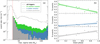 |
Fig. B.3 Results of the meteor trigger algorithm on the first nine data-taking sessions of Mini-EUS0. (a) Histogram of the maximal sigma ratio (Rxy, Eq. B.4) for all triggers (black line) and for the three classes of events (meteors, M – green; other events, U – blue; false positives, N – grey). (b) Percentage of M, U, and N events as a function of the moon phase for each session (coloured points) over which the solid lines plot a least-square linear fit together with its 68% confidence interval. |
 |
Fig. B.4 Maps of the positions of the nominal central point of the Mini-EUSO FOV, projected on the ground, corresponding to the starting GTU of triggered events of sessions no. 05-14 for the three following classes: (a) meteors, M – green; (b) other events, U – blue; (c) false positives, N – grey. Panel d plots a magnification of the map over Central and Southern Europe and North Africa. |
We also studied the performance of our meteor trigger in varying background illumination conditions. In each session, these conditions can vary significantly due to the observed region on the ground, as well as the cloud coverage and the reflected and stray light from the Sun and Moon. Starting from the analysis of D3 data of Mini-EUSO, Casolino et al. (2023) carried out a detailed study of the night-time emission of the Earth in the near-UV wavelength range. The average counts for cloud-free observations vary from ~0.6 cnts GTU−1 during a new moon to ~40 cnts GTU−1 during a full moon (also depending on the Moon’s elevation above the local horizon). The effect of this variability can be observed in Fig. B.3b, which plots the fraction of events for the three classes M, U, and N as a function of the moon phase. The percentage of identified meteors of the whole trigger ensemble varies from about 70% during a new moon down to just a few percent in case of a full moon. On the other hand, the fraction of both non-meteor events and false positives increases with the increasing of the moon phase values, from 5% to 30% for U and from 20% to 60% for N events, respectively, for new and full moon conditions. Moreover, Fig. B.4 shows on the globe the positions of the triggered events for each class. Overall, 49% of events are triggered on land and 51% over the oceans. This distribution varies if we consider only meteor events, which are more likely triggered over the oceans (66%) rather than on land (34%). The opposite is true for U and N events, which are more frequent on land (63%) and less over the oceans (37%). This is best shown in Fig. B.4d, which reports a magnification of the map over Europe and North Africa. From this figure, it is evident that false positives are very often triggered over densely populated and, therefore, highly light-polluted areas, such as the whole of Western Europe and the coast of North Africa facing the Mediterranean Sea. On the other hand, N events are rarely triggered over the Mediterranean Sea, the Atlantic Ocean and darker regions on dry land, such as the Sahara Desert.
B.2 Trigger 2
The trigger logic described in Appendix B.1 was originally designed for the onboard detection of space debris in future missions of the JEM-EUSO programme. Since the beginning of the Mini-EUSO data acquisition, an alternative trigger method, specifically devoted to the offline detection of meteors, has been developed as well. The main steps of this trigger are described below and summarised in Fig. B.5.
The first step of the algorithm is to identify the moments in which each EC unit switches between cathode-3 and cathode-2 modes. The data is then divided into sections with the same efficiency and corresponding to these modes, while removing a few frames of noisy transition periods as well as sections shorter than eight frames. The next step is to find meteor-like peaks for each pixel in each data section. This task is not straightforward because of the uneven response of the Mini-EUSO detector and the complex variability of natural background light mainly due to sources moving on the ground with a non-point-like PSF. Initially, the short-period fluctuations are eliminated with a wavelet filter that decomposes the signal into seven levels with a stationary sym2 wavelet transform, thus reconstructing it by ignoring the highest and most fluctuating level. The sym2 wavelet was chosen empirically, from a set of PyWavelets wavelets (Lee et al. 2019), being the one showing the best signal-to-noise ratio after filtering for selected meteor events. The local background is then calculated on the filtered signal using a TSpectrum class belonging to the ROOT framework (Brun & Rademakers 1997). The parameters of both steps are tuned to follow the time variability of the background induced by on-ground moving sources, while simultaneously ignoring shorter spikes caused by meteor candidates. The initial removal of the shortest period variability significantly improves the results obtained with TSpectrum in the subsequent step. Then, the significance of each data point is calculated by subtracting the average and dividing by the standard deviation (i.e. the square root, see Sect. 4.4) of the pixel data section. This part of the algorithm returns a list of time-space coordinates (x, y, t) of data points that exceed the significance of 5σ, similar to the trigger method described in Appendix B.1.
 |
Fig. B.5 Main steps of the alternative meteor trigger method (trigger 2), detailed in Appendix B.2. |
Data points that come from known noisy parts of the detector are removed from this list, together with solitary triggers that do not have a counterpart in a 4 GTU window and are thus unlikely to be meteors. Then, the single-pixel single-frame triggers are grouped into multi-pixel multi-frame events. For this purpose, the algorithm clusters triggers that are separated from other group members by at least five frames or pixels. This operation is performed using the query_ball_tree function of SciPy spatial. cKDTree (Virtanen et al. 2020) and a function that joins the clusters with at least a single common element.
At this stage, the list of events should be free of most fluctuations of the detector, but still encloses many real events that are not meteors. Therefore, the next step of the algorithm is to categorise the events with simple, consecutive checks. The categories are: single and two-frame events; stationary events; events occupying most of the PDM; events with erratic movement; slow and vertically moving events (ground sources); events lasting longer than 40 frames; scattered events; and meteor candidates. The latter are the events that did not fall into the previous categories. These candidates are subject to the following more detailed cuts:
Light curve shape: checking the dependencies between light curve parameters of the pixels of the event, such as peak height over peak prominence and width over prominence, calculated with SciPy signal.find_peaks function;
Density: discarding events with too low density, which is defined either as the number of pixels over the width of the event in the x direction (the same in y) or as the number of pixels over the bounding rectangle;
Compactness: discarding diffuse events with a low ratio between the maximal pixel value and the number of pixels in the event.
The first cut tries to ensure that the light curves of the pixels of the event have the characteristics of those created by a fast-moving point source. The other two cuts focus on the shape of the candidate event, which should be described by the PSF of the detector in the case of a meteor signal. This is not true, for example, in the case of thunderstorm discharges and non-pointlike ground sources.
After these steps, this algorithm also allows for a rough estimation, with simple and quick methods, of basic meteor properties such as light curve, track on the PDM and speed, which are then stored in a database of triggered events. These measurements are not discussed here because, among other reasons, their quality could be significantly improved. In particular, for very dim meteors, an imperfect background subtraction has a considerable negative impact on the quality of such measurements. However, this quick estimation serves well the purpose of showing the general properties of the dataset and identifying interesting events among bright candidates.
This algorithm allowed for the detection of thousands of meteors in the Mini-EUSO data (see Sect. 4.1). However, depending on the characteristics of the data-taking session, between 10% and 30% of the candidates are confirmed to not be meteors according to a dedicated double-blind check visual inspection. In addition, this algorithm does not detect a significant portion of the meteors detected by the other trigger presented in Sect. B.1. Similarly to what we discussed for the first algorithm, the event types that are most difficult to distinguish from meteors are signals from background fluctuations and ground sources remaining after the imperfect background subtraction. For the same reason, many meteor candidates are either contaminated with spurious pixels or stripped of essential data points. These imperfections are easily noticeable to the human eye, most likely because of the interplay of many light curve parameters that are difficult to describe in an algorithm, but that could be well characterised by deep neural networks. Their implementation in the algorithm could allow the fast detection of many more meteors with much cleaner signals, as well as a much more straightforward classification of event types, thus reducing the need for fine-tuned specialistic cuts as the ones presented in this section.
Appendix C Computation of the exposure of the Mini-EUSO telescope
In this appendix, we provide a short description of the simulations developed for the computation of the exposure of the Mini-EUSO telescope, as introduced in Sect. 5. The details of these simulations will be given in a forthcoming publication.
The dynamical evolution of the meteor event within the Earth’s atmosphere is described by a set of differential equations that summarise the main physical phenomena involved in the process. Following the description of Bronshten (1983), in the hypothesis of intensive evaporation, the aforementioned equations can be given as:
 (C.1)
(C.1)
which are, respectively, the altitude, deceleration, mass-loss (ablation) and intensity equations. In Eq. C.1, H is the altitude of the meteor from the ground, V is the apparent speed module of the meteoroid, M is the mass of the meteoroid, S is the area of its cross-section (perpendicular to the motion direction), and I is the light intensity emitted by the meteor (all as a function of the time t). The other quantities are the physical parameters of the meteor and they are, respectively, the trajectory inclination with respect to the ground (γ), the atmospheric drag coefficient (Γ), the atmospheric density (ρa), the ablation coefficient (σ), and the luminous efficiency (τ). The mass-loss equation can be easily solved as:
 (C.2)
(C.2)
where M∞ and V∞ are, respectively, the pre-atmospheric mass and speed of the meteoroid. Furthermore, the deceleration equation can be solved quasi-analytically according to the approach of Gritsevich (2009); Gritsevich & Koschny (2011) as:
![Mathematical equation: $h = \ln (2\alpha ) + \beta - \ln \left[ {Ei(\beta ) - Ei\left( {\beta {v^2}} \right)} \right],$](/articles/aa/full_html/2024/07/aa49236-24/aa49236-24-eq30.png) (C.3)
(C.3)
where Ei(x) is the exponential integral function, h = H/H0 is the height of the meteor normalised to the scale height of the atmosphere, v = V/V∞ is the speed normalised to the pre-atmospheric value, while α and β are two dimensionless coefficients that enclose most of the physical parameters listed above (respectively, the ballistic coefficient and the mass-loss parameter, see Gritsevich 2009). Finally, the altitude equation can be numerically integrated, given the profile speed V = V(H) that can be derived from Eq. C.3, and the intensity equation can be either solved numerically or according to Eq. 14 of Gritsevich & Koschny (2011).
To simulate each event, all the parameters included in Eq. C.1 are randomly sorted over a distribution representing the whole ensemble of meteors potentially observable from Mini-EUSO, following an approach similar to the one presented in Bouquet et al. (2014). In particular, the pre-atmospheric mass value M∞ is chosen according to the desired minimum absolute magnitude ℳ of the meteor that is to be simulated. The dynamics of the event is finally reported as seen by the Mini-EUSO telescope, located at an altitude of 420 km from the ground, by implementing the PSF response of each MAPMT and the apparent motion of the ISS along the y axis of the PDM. An example of the results of these simulations is presented in Fig. C.1 in the case of a meteorwith ℳ = +3.5, due to the atmospheric entry ameteoroid with mass of M∞ = 0.02 g, at a speed of V∞ = 66.6 km s−1, and with an inclination angle of γ = 39.6°. Since, in this example, the apparent motion of the meteor on the PDM started at the corners between four MAPMTs, a significant fraction of counts was lost during the first 10 GTU (panel f, red curve). However, the maximum value of the light curve of ~0.35 cnts GTU−1 (defining the peak absolute magnitude ℳ) corresponded to the centre of the MAPMT and was correctly recorded by the instrument.
As introduced in Sect. 5, this simulation was run for 2000 meteors every 0.5 mag for ℳ ∊ [−2,8] and the produced events were, therefore, reported on a variable background level on the PDM b ∊ [10−1, 102] cnts GTU−1 added to a component of Poissonian noise. In so doing, we selected 300 events for each (ℳ, b) combination. Through this process, we can estimate a value for the trigger efficiency, ∊(ℳ, b), by running the trigger and postprocessing analysis (see Sect. 3.1 and 3.2) over the simulated ensemble of meteors and by counting how many of them are triggered with respect to the total number for each combination of (ℳ, b). These tabulated values are finally scaled to the Mini-EUSO D3 data by considering a pixel-wise time average over δt = 25 GTU (~ 1 s) across the considered sessions,
 (C.4)
(C.4)
adding up the contributions of each pixel weighted by its projected area at 100 km of altitude from the ground to compute the total exposure for each ℳ value. This time interval δt is larger than the expected maximum duration of the signal of a meteor over the single pixel (20 GTU, see Sect. 3.3), thus allowing for the contribution of fast transient signals (like meteors) to be averaged. At the same time, δt corresponds to an apparent motion of fixed ground sources confined to the approximate pixel dimension. While computing the total exposure, ECs in cathode-2 mode are excluded because they correspond to a much lower photon collection efficiency of the instrument. In order to account for this, we scan the pixels within each EC on the PDM and check, over each D3 frame, for the following condition: Cxy < 10−3 cnts GTU−1. If more than 15 pixels display such a low count value, we consider that the corresponding EC is in cathode-2 mode for that time interval. Then, for each ti, we define a matrix Ωxy(ti) that encloses the fraction of GTUs for which each pixel (x, y) was found in cathode-3 (with respect to the total, i.e. 25 GTU). Therefore, the exposure of Mini-EUSO (for each D3 data file) as a function of the absolute magnitude can be given as:
![Mathematical equation: $X({\cal M}) = {A_{px}}\delta t\mathop {\mathop \sum \nolimits^ }\limits_{{t_i}} \sum\limits_{x,y}^{{\rm{PDM}}} {{{\rm{\Omega }}_{xy}}\left( {{t_i}} \right)} \left[ {{\cal M},{{{b_{xy}}\left( {{t_i}} \right)} \over {{S_{xy}}}}} \right],$](/articles/aa/full_html/2024/07/aa49236-24/aa49236-24-eq32.png) (C.5)
(C.5)
where Apx is the equivalent average area of one pixel and accounts for the sum over (x, y) on the PDM. This computation was performed to estimate the efficiency of trigger 1 (Sect. 3.1, Fig. 9). Therefore, we select the events detected by this method, which are ~14.4 thousand (60% of the 24 thousand total events, see Table 1). The analysis of the performance of trigger 2 will be included in a forthcoming publication.
 |
Fig. C.1 Example of simulated meteor of minimum absolute magnitude ℳ = +3.5 as seen by the Mini-EUSO telescope. The meteoroid had a pre-atmospheric mass of M∞ = 0.02 g and entered the atmosphere at V∞ = 66.6 km s−1 with an inclination angle of γ = 39.6°. (a) Altitude from the ground as a function of time; (b) speed module; (c) absolute magnitude light curve, peaking at +3.5; (d) map of pixels on the PDM that were crossed by the signal of the meteor; (e) single-pixel light curves with the colour code of panel d; (f) total integrated light curve (black curve, inverse of Eq. 7 from panel c) compared to the actual counts recorded on the PDM (red curve), which are lower in the first part of the event because the apparent path of the meteor crossed the corner between four MAPMTs. |
From a visual inspection of the resulting flux density plot presented in Fig. 10, a decreasing slope of the result of Mini-EUSO is evident at the lower end of the distribution for M∞ < 10−5 kg. This evidence may be due to a residual overestimation of the instrument exposure for the population of these faint events. We are currently testing an alternative approach for the exposure computation that directly implements the simulated meteors over the observed D3 data during all the considered sessions. This work requires a remarkable computational effort, since we are dealing with a set of ~5.7 days of observation sampled at 40.96 ms resolution. On the other hand, such an approach represents a more general solution and does not require any further assumptions on the response of the detector, the counting statistics and the flat-field normalisation. Figure C.2 presents some preliminary results of the comparison of X(M) when using the two aforementioned approaches and considering the data of Mini-EUSO acquired along three ISS orbits during session no. 08. This comparison points out a general agreement of these two methods within ~20 % of relative accuracy (at least for ℳ ≤ +5, i.e. the limit chosen for the meteor flux computation, as reported in Sect. 5). In this figure, the red curves plot the results assuming a flat background (method 1, Eq. C.5) and the black dots with error bars are computed through this alternative approach (method 2). The best agreement between the two is reached for orbit 7 (panels c and f), which, for most of the orbit, corresponds to the transit of the ISS over South America and the Atlantic Sea. A more significant difference was highlighted in the case of the background D3 maps being highly variable within the FOV of Mini-EUSO and over time. This case usually corresponds to the transit of Mini-EUSO over cities and, more generally, over densely populated areas (e.g. orbit 1 and 2). In particular, the results of the flat background assumption appear to overestimate the trigger efficiency for ℳ ≤ +5. A possible explanation of this mismatch is that a significant variation of the background counts within short time intervals (< 1 s) may neg atively affect the progressive adjustment of the threshold value of the trigger (Eq. B.3). However, this effect is not considered within the simulations presented in Sect. 5, for which we make the assumption that Cxy does not vary significantly along the fixed time interval of δt = 1 s.
 |
Fig. C.2 Results of the comparison between two methods to compute the total exposure of the Mini-EUSO telescope, as applied to the observation of meteors in the magnitude range ℳ ∊ [−2, 8] for three ISS orbits during session no. 08 (30-31 December 2019). In all panels, the red curve plots the total exposure computed from the flat background assumption on each pixel (method 1, Eq. C.5), whereas the black dots with error bars are the results of the direct implementation of meteor simulations over the observed D3 data of this sessions, once all recorded meteors are artificially removed from the video (method 2). Panels a-c plot the comparison between methods 1 and 2 for orbits 1, 2, and 7 of session no. 08 and panels d-f report the ratio between the two methods (i.e. the factor that should be applied to the absolute flux of meteors if considering the exposure resulting from method 2 instead of method 1). |
Appendix D Exposure of Mini-EUSO as a function of the meteoroid mass
In order to implement the computation of the pre-atmospheric mass of the meteoroid according to Eq. 17, the first step is the estimation of the radiant flux, I(t), namely the power emitted by each observed meteor in the bandpass of Mini-EUS0. In particular, we are interested in the total radiated energy, Erad, over the whole duration of the event, which can be given as a function of the absolute magnitude, ℳ(t), from Eq. 7 as follows:
 (D.1)
(D.1)
where ƒλ and ∆λ are the zero-point flux and width of the Mini-EUSO bandpass (see Eq. 6), d = 100 km is the reference distance for the definition of the absolute magnitude of meteors, δtD3 is the D3 time resolution, and the index k refers to D3 frames within the duration ∆t of the event. Furthermore, it is useful to estimate a conversion between Erad and the minimum absolute magnitude, ℳ = min{ℳ(t)}. This conversion is needed because the exposure X of Mini-EUSO for the observation of meteors was estimated as a function of M. In our case, we found that this can be approximated with a linear regression as:
 (D.2)
(D.2)
where the uncertainty of the intercept refers to the 68% confidence interval.
To estimate the absolute flux of meteors as a function of the meteoroid mass, we started from the histogram of the pre-atmospheric mass, M∞ , of the events observed by Mini-EUSO and computed according to Eq. 17. The total radiated energy, Erad, is given by Eq. D.1, where V∞ is estimated from the observed horizontal speed, V, assuming that the inclination angle is distributed according to Eq. 16 and the luminous efficiency, τ = τ(V∞), is provided by one of the formulations presented in Sect. 5.2. In order to correct this histogram for the observational bias, we then need to estimate the exposure, X, of Mini-EUSO to the observation of meteors as a function of M∞ . This can be translated from the expression of X = X(ℳ) discussed in Appendix C by adapting the debiasing approach introduced by Koschny et al. (2017) to our case, which is summarised as follows:
For each bin, i → M∞,i, of the mass histogram, we consider the underlying theoretical speed distribution, ρt(V∞), of meteoroids reported at an altitude of 100 km from the ground, given by ECSS (2008) and assumed to be independent from the meteoroid mass.
-
As a function of V∞, in the domain of ρt, the total radiated energy, Erad,i, is given by the inverse of Eq. 17. Then, assuming Eq. D.2, we can estimate the absolute magnitude, ℳi(V∞), as a function of the pre-atmospheric speed and, in particular, the corresponding detection efficiency, ∊i(V∞), can be given as:
![Mathematical equation: ${_i}\left( {{V_\infty }} \right) = {{X\left[ {{{\cal M}_i}\left( {{V_\infty }} \right)} \right]} \over {{X_{{\rm{nom}}}}}},$](/articles/aa/full_html/2024/07/aa49236-24/aa49236-24-eq35.png) (D.3)
(D.3)where X(ℳ) is computed according to Eq. C.5 and Xnom is the nominal exposure, that is: not considering the effect of the trigger inefficiency. For the dataset of Mini-EUSO observations discussed in this paper, Xnom ≃ 975 yr km2.
-
Therefore, we can estimate the observable speed distribution of meteors for each mass bin, M∞,i as:
 (D.4)
(D.4)An example of ρi(V∞) compared to ρt(V∞) is given in Fig. D.1 for M∞ = 10−4.3 kg assuming the luminous efficiency of Ceplecha & McCrosky (1976).
Finally, the exposure for each mass bin, M∞,i, is proportional to the ratio of the integrals of the observed and theoretical speed distributions:
 (D.5)
(D.5)
This computation is repeated for each formulation of τ = τ(V∞) presented in Sect. 5.2 and it is integrated into a bootstrap process to propagate known uncertainties in the problem, such as the one affecting the conversion of Eq. D.2 and the 20% relative uncertainty of X(ℳ). An example of the result of this process for the luminous efficiency formulation of Ceplecha & McCrosky (1976) is shown in Fig. D.2.
In Sect. 5.2, we discussed that a residual bias is likely evident from the resulting flux distribution reported in Fig. 11b-f, approximately in the half interval of smaller masses for all cases. Such evidence may be due to secondary effects that are not taken into account in the methodology presented here for the estimation of the exposure as a function of the meteoroid mass. For example, Eq. D.3 accounts for the dependence of the detection efficiency, ∊, from the meteor speed but only according to the scaling of the luminosity of the event to V∞. However, the trigger might exhibit an efficiency variation intrinsically related to the apparent speed on the object projected on the PDM of Mini-EUS0. A preliminary study of this effect highlighted a decreasing value of ∊ for slow-moving events because they can be mistaken by the trigger as stationary sources and therefore be excluded. A similar effect is present for the detection of very fast-moving meteors, since, in this case, the signal of the PSF spreads on multiple pixels on each frame. Furthermore, Fig. 11b-f shows that the relative displacement of the estimated flux density from the expected linear trend is different for the various models of the luminous efficiency. This evidence suggests that the scaling of luminous efficiency according to V∞ is also quite relevant to this correction, besides the fact that, as already mentioned, the average value of τ causes the shift of the flux density plot in a variable mass range.
 |
Fig. D.1 Example of the distributions of the pre-atmospheric speed, V∞, of meteoroids at 100 km altitude from the ground, used for the estimation of the exposure of Mini-EUSO as a function of the meteoroid mass, M∞. The black line plots the assumed theoretical distribution, ρt, given by ECSS (2008) and the green line reports the distribution of meteoroids, ρi, for M∞ = 10−4.3 kg observable by Mini-EUSO if assuming the luminous efficiency, τ = τ(V∞), given by Ceplecha & McCrosky (1976). For this mass bin, the exposure of Mini-EUSO is estimated to be Xi ≃ 0.68Xnom from Eq. D.5. |
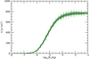 |
Fig. D.2 Exposure X of the Mini-EUSO telescope as a function of the pre-atmospheric mass of the meteoroids, M∞ , estimated thanks to the methodology described in Appendix D and according to the formulation of the luminous efficiency of Ceplecha & McCrosky (1976). The green points report the result of the bootstrap ensemble of 100 repetitions and their spread highlights the uncertainty in the determination of the exposure. The thick green line plots the ensemble mean and the green band reports the 68% confidence interval estimated through the ensemble standard deviation for each mass bin. |
References
- Abdellaoui, G., Abe, S., Acheli, A., et al. 2017, Planet. Space Sei., 143, 245 [NASA ADS] [CrossRef] [Google Scholar]
- Abdellaoui, G., Abe, S., Adams, J. H., et al. 2018, Astropart. Phys., 102, 98 [NASA ADS] [CrossRef] [Google Scholar]
- Abdellaoui, G., Abe, S., Adams, J. H., et al. 2024, Astropart. Phys., 154, 102891 [NASA ADS] [CrossRef] [Google Scholar]
- Abe, S., Adams, J. H., Allard, D., et al. 2023, Eur. Phys. J. C, 83, 1028 [NASA ADS] [CrossRef] [Google Scholar]
- Adams, J. H., Ahmad, S., Albert, J. N., et al. 2013, Astropart. Phys., 44, 76 [NASA ADS] [CrossRef] [Google Scholar]
- Adams, J. H., Ahmad, S., Albert, J. N., et al. 2015a, Exp. Astron., 40, 253 [NASA ADS] [CrossRef] [Google Scholar]
- Adams, J. H., Ahmad, S., Albert, J. N., et al. 2015b, Exp. Astron., 40, 239 [NASA ADS] [CrossRef] [Google Scholar]
- Adams, J. H., Ahmad, S., Albert, J. N., et al. 2015c, Exp. Astron., 40, 153 [NASA ADS] [CrossRef] [Google Scholar]
- Adams, J. H. Jr, Anchordoqui, L. A., Apple, J. A., et al. 2017, arXiv e-prints [arXiv:1703.04513] [Google Scholar]
- Adams, J. H., Ahmad, S., Allard, D., et al. 2022, Space Sci. Rev., 218, 3 [CrossRef] [PubMed] [Google Scholar]
- Bacholle, S., Barrillon, P., Battisti, M., et al. 2021, ApJS, 253, 36 [CrossRef] [Google Scholar]
- Barrillon, P., Battisti, M., Belov, A., et al. 2023, Exp. Astron., 55, 569 [NASA ADS] [CrossRef] [Google Scholar]
- Battisti, M., Barghini, D., Belov, A., et al. 2022, Adv. Space Res., 70, 2750 [NASA ADS] [CrossRef] [Google Scholar]
- Battisti, M., Bertaina, M., Arnone, E., Sammartino, G., & Pretto, G. 2023, arXiv e-prints [arXiv:2309.11920] [Google Scholar]
- Bellot Rubio, L. R. 1994, WGN, J. Int. Meteor Organ., 22, 118 [Google Scholar]
- Belov, A., Bertaina, M., Capel, F., et al. 2018, Adv. Space Res., 62, 2966 [NASA ADS] [CrossRef] [Google Scholar]
- Bisconti, F., Miyamoto, H., Barghini, D., et al. 2022, Exp. Astron., 53, 133 [NASA ADS] [CrossRef] [Google Scholar]
- Blaauw, R. C., Campbell-Brown, M. D., & Weryk, R. J. 2011, MNRAS, 412, 2033 [NASA ADS] [CrossRef] [Google Scholar]
- Bland, P. A., Smith, T. B., Jull, A. J. T., et al. 1996, MNRAS, 283, 551 [Google Scholar]
- Bottke, W. F., Durda, D. D., Nesvorný, D., et al. 2005, Icarus, 179, 63 [Google Scholar]
- Bouquet, A., Baratoux, D., Vaubaillon, J., et al. 2014, Planet. Space Sci., 103, 238 [Google Scholar]
- Bradley, J. P. 2003, Treatise Geochem., 1, 711 [NASA ADS] [Google Scholar]
- Bronshten, V. A. 1983, Physics of Meteoric Phenomena (Springer Link) [Google Scholar]
- Brown, P., Spalding, R. E., ReVelle, D. O., Tagliaferri, E., & Worden, S. P. 2002, Nature, 420, 294 [Google Scholar]
- Brownlee, D. E. 2001, in Accretion of Extraterrestrial Matter Throughout Earth’s History, 1 [Google Scholar]
- Brun, R., & Rademakers, F. 1997, Nucl. Instrum. Methods Phys. Res. A, 389, 81 [CrossRef] [Google Scholar]
- Capel, F., Belov, A., Cambiè, G., et al. 2019, J. Astron. Telesc. Instrum. Syst., 5, 044009 [CrossRef] [Google Scholar]
- Carbary, J. F., Morrison, D., Romick, G. J., & Yee, J. H. 2003, Icarus, 161, 223 [NASA ADS] [CrossRef] [Google Scholar]
- Casolino, M., Klimov, P., & Piotrowski, L. 2017, Prog. Theor. Exp. Phys., 2017, 12A107 [CrossRef] [Google Scholar]
- Casolino, M., Barghini, D., Battisti, M., et al. 2023, Remote Sens. Environ., 284, 113336 [CrossRef] [Google Scholar]
- Ceplecha, Z., & McCrosky, R. E. 1976, J. Geophys. Res., 81, 6257 [NASA ADS] [CrossRef] [Google Scholar]
- Ceplecha, Z., Borovicka, J., Elford, W. G., et al. 1998, Space Sci. Rev., 84, 327 [NASA ADS] [CrossRef] [Google Scholar]
- Cevolani, G., & Gabucci, M. F. 1996, Nuovo Cimento C Geophys. Space Phys., 19C, 271 [CrossRef] [Google Scholar]
- Colas, F., Zanda, B., Bouley, S., et al. 2020, A&A, 644, A53 [EDP Sciences] [Google Scholar]
- Colonna, G., Capitelli, M., & Laricchiuta, A. 2019, Hypersonic Meteoroid Entry Physics [CrossRef] [Google Scholar]
- Cziczo, D. J., Thomson, D. S., & Murphy, D. M. 2001, Science, 291, 1772 [NASA ADS] [CrossRef] [Google Scholar]
- Devillepoix, H. A. R., Cupák, M., Bland, P. A., et al. 2020, Planet. Space Sci., 191, 105036 [Google Scholar]
- Dohnanyi, J. S. 1967, ApJ, 149, 735 [NASA ADS] [CrossRef] [Google Scholar]
- Dohnanyi, J. S. 1969, J. Geophys. Res., 74, 2531 [Google Scholar]
- Drolshagen, G., Koschny, D., Drolshagen, S., Kretschmer, J., & Poppe, B. 2017, Planet. Space Sci., 143, 21 [NASA ADS] [CrossRef] [Google Scholar]
- Drouard, A., Gattacceca, J., Hutzler, A., et al. 2019, Geology, 47, 673 [Google Scholar]
- ECSS. 2008, European Cooperation for Space Standardization, Space Engineering, Space Environment, Tech. Rep. ECSS-E-ST-10-04C, ESA/ESTEC, Noordwjik, Netherlands [Google Scholar]
- Erickson, J. E. 1968, J. Geophys. Res., 73, 3721 [CrossRef] [Google Scholar]
- Evatt, G. W., Smedley, A. R. D., Joy, K. H., et al. 2020, Geology, 48, 683 [NASA ADS] [CrossRef] [Google Scholar]
- Foschini, L. 1999, in 2nd National Meeting of Planetary Sciences, Bormio (Italy) 25-31 January 1998. Proceedings, 131 [Google Scholar]
- Galligan, D. P., & Baggaley, W. J. 2004, MNRAS, 353, 422 [NASA ADS] [CrossRef] [Google Scholar]
- Gardiol, D., Barghini, D., Buzzoni, A., et al. 2021, MNRAS, 501, 1215 [Google Scholar]
- Gattacceca, J., Valenzuela, M., Uehara, M., et al. 2011, Meteorit. Planet. Sci., 46, 1276 [NASA ADS] [CrossRef] [Google Scholar]
- Granvik, M., & Brown, P. 2018, Icarus, 311, 271 [Google Scholar]
- Gritsevich, M. I. 2009, Adv. Space Res., 44, 323 [NASA ADS] [CrossRef] [Google Scholar]
- Gritsevich, M., & Koschny, D. 2011, Icarus, 212, 877 [CrossRef] [Google Scholar]
- Grun, E., Zook, H. A., Fechtig, H., & Giese, R. H. 1985, Icarus, 62, 244 [NASA ADS] [CrossRef] [Google Scholar]
- Halliday, I. 2001, in Accretion of Extraterrestrial Matter Throughout Earth’s History, 305 [CrossRef] [Google Scholar]
- Halliday, I., Griffin, A. A., & Blackwell, A. T. 1996, Meteorit. Planet. Sci., 31, 185 [Google Scholar]
- Hawkins, G. S., & Upton, E. K. L. 1958, ApJ, 128, 727 [NASA ADS] [CrossRef] [Google Scholar]
- Hill, K. A., Rogers, L. A., & Hawkes, R. L. 2005, A&A, 444, 615 [NASA ADS] [CrossRef] [EDP Sciences] [Google Scholar]
- Hutzler, A., Gattacceca, J., Rochette, P., et al. 2016, Meteorit. Planet. Sci., 51, 468 [Google Scholar]
- Janches, D., Brunini, C., & Hormaechea, J. L. 2019, AJ, 157, 240 [NASA ADS] [CrossRef] [Google Scholar]
- Jenniskens, P., Tedesco, E., Murthy, J., Laux, C. O., & Price, S. 2002, Meteorit. Planet. Sci., 37, 1071 [NASA ADS] [CrossRef] [Google Scholar]
- Jenniskens, P., Albers, J., Tillier, C. E., et al. 2018, Meteorit. Planet. Sci., 53, 2445 [NASA ADS] [CrossRef] [Google Scholar]
- Jenniskens, P., Utas, J., Yin, Q.-Z., et al. 2019, Meteorit. Planet. Sci., 54, 699 [Google Scholar]
- Kasuga, T., Watanabe, J., & Ebizuka, N. 2005, A&A, 438, L17 [NASA ADS] [CrossRef] [EDP Sciences] [Google Scholar]
- Klimov, P. A., Panasyuk, M. I., Khrenov, B. A., et al. 2017, Space Sci. Rev., 212, 1687 [Google Scholar]
- Klimov, P., Battisti, M., Belov, A., et al. 2022, Universe, 8, 88 [CrossRef] [Google Scholar]
- Kornoš, L., Koukal, J., Piffl, R., & Tóth, J. 2014, in Proceedings of the International Meteor Conference, Poznan, Poland, 22-25 August 2013, eds. M. Gyssens, P. Roggemans, & P. Zoladek, 23 [Google Scholar]
- Koschack, R., & Rendtel, J. 1990, WGN, J. Int. Meteor Organ., 18, 119 [NASA ADS] [Google Scholar]
- Koschny, D., & Zender, J. 1998, Earth Moon Planets, 82, 209 [NASA ADS] [CrossRef] [Google Scholar]
- Koschny, D., Drolshagen, E., Drolshagen, S., et al. 2017, Planet. Space Sci., 143, 230 [NASA ADS] [CrossRef] [Google Scholar]
- Kruijer, T. S., Kleine, T., & Borg, L. E. 2020, Nat. Astron., 4, 32 [Google Scholar]
- Landolt, A. U. 2009, AJ, 137, 4186 [Google Scholar]
- Lee, G., Gommers, R., Waselewski, F., Wohlfahrt, K., & O’Leary, A. 2019, J. Open Source Softw., 4, 1237 [NASA ADS] [CrossRef] [Google Scholar]
- Levenberg, K. 1944, Q. Appl. Math., 2, 164 [Google Scholar]
- Marcelli, L., Arnone, E., Barghini, M., et al. 2022, in 37th International Cosmic Ray Conference, 12-23 July 2021, Berlin, 367 [Google Scholar]
- Marcelli, L., Barghini, D., Battisti, M., et al. 2023, Rendiconti Lincei. Sci. Fisiche Natur., 34, 23 [NASA ADS] [CrossRef] [Google Scholar]
- Markwardt, C. B. 2009, in Astronomical Data Analysis Software and Systems XVIII, eds. D. A. Bohlender, D. Durand, & P. Dowler, ASP Conf. Ser., 411, 251 [NASA ADS] [Google Scholar]
- Marquardt, D. W. 1963, J. Soc. Ind. Appl. Math., 11, 431 [Google Scholar]
- Miyamoto, H., Battisti, M., Belov, A. S., et al. 2019, in 36th International Cosmic Ray Conference (ICRC2019), 253 [Google Scholar]
- Miyamoto, H., et al. 2023, EPJ Web Conf., 283, 06017 [NASA ADS] [CrossRef] [EDP Sciences] [Google Scholar]
- Montanaro, A., Ebisuzaki, T., & Bertaina, M. 2022, J. Space Saf. Eng., 9, 72 [NASA ADS] [CrossRef] [Google Scholar]
- Moorhead, A. V., & Matney, M. 2021, Adv. Space Res., 67, 384 [NASA ADS] [CrossRef] [Google Scholar]
- Moré, J. J. 1978, in Numerical Aanalysis (Springer), 105 [Google Scholar]
- Oberst, J., Molau, S., Heinlein, D., et al. 1998, Meteorit. Planet. Sci., 33 [Google Scholar]
- Olinto, A. V., Krizmanic, J., Adams, J. H., et al. 2021, J. Cosmol. Astropart. Phys., 2021, 007 [Google Scholar]
- Olivi, L., Bertaina, M., Montanaro, A., et al. 2023, Remote Sens., submitted [Google Scholar]
- Piotrowski, L., Barghini, D., Battisti, M., et al. 2022, in 37th International Cosmic Ray Conference, 503 [Google Scholar]
- Plebaniak, Z., Karczmarczyk, J., Marszal, W., et al. 2017, in 35th International Cosmic Ray Conference, 301, (ICRC2017), 378 [Google Scholar]
- Pokorný, P., & Brown, P. G. 2016, A&A, 592, A150 [NASA ADS] [CrossRef] [EDP Sciences] [Google Scholar]
- Rietmeijer, F. J. M., Della Corte, V., Ferrari, M., Rotundi, A., & Brunetto, R. 2016, Icarus, 266, 217 [Google Scholar]
- Rigby, J., Perrin, M., McElwain, M., et al. 2023, PASP, 135, 048001 [NASA ADS] [CrossRef] [Google Scholar]
- Robertson, J. B., & Ayers, W. G. 1968, Photometry of an Iron Artificial Meteor Reentering at 11 Kilometers Per Second (National Aeronautics and Space Administration) [Google Scholar]
- Rojas, J., Duprat, J., Engrand, C., et al. 2021, Earth Planet. Sci. Lett., 560, 116794 [CrossRef] [Google Scholar]
- Ryabova, G. O., Asher, D. J., & Campbell-Brown, M. J. 2019, Meteoroids: Sources of Meteors on Earth and Beyond, (Cambridge: Cambridge University Press) [CrossRef] [Google Scholar]
- Simek, M., & McIntosh, B. A. 1968, in Physics and Dynamics of Meteors, 33, eds. L. Kresak, & P. M. Millman, 362 [Google Scholar]
- Smith, J. C., Morris, R. L., Rumpf, C., et al. 2021, Icarus, 368, 114576 [CrossRef] [Google Scholar]
- Spurný, P., Borovicka, J., Mucke, H., & Svoren, J. 2017, A&A, 605, A68 [NASA ADS] [CrossRef] [EDP Sciences] [Google Scholar]
- Suggs, R. M., Moser, D. E., Cooke, W. J., & Suggs, R. J. 2014, Icarus, 238, 23 [NASA ADS] [CrossRef] [Google Scholar]
- Tagliaferri, E., Spalding, R., Jacobs, C., Worden, S. P., & Erlich, A. 1994, in Hazards Due to Comets and Asteroids, 199 [Google Scholar]
- Thomas, R. M., Whitham, P. S., & Elford, W. G. 1988, J. Atmos. Sol. Terr. Phys., 50, 703 [NASA ADS] [CrossRef] [Google Scholar]
- Unsalan, O., Jenniskens, P., Yin, Q.-Z., et al. 2019, Meteorit. Planet. Sci., 54, 953 [NASA ADS] [CrossRef] [Google Scholar]
- Verniani, F. 1973, J. Geophys. Res., 78, 8429 [CrossRef] [Google Scholar]
- Vida, D., Campbell-Brown, M., Brown, P. G., Egal, A., & Mazur, M. J. 2020, A&A, 635, A153 [NASA ADS] [CrossRef] [EDP Sciences] [Google Scholar]
- Vida, D., Blaauw Erskine, R. C., Brown, P. G., et al. 2022, MNRAS, 515, 2322 [NASA ADS] [CrossRef] [Google Scholar]
- Virtanen, P., Gommers, R., Oliphant, T. E., et al. 2020, Nat. Methods, 17, 261 [Google Scholar]
- Warren, J. L., & Zolensky, M. E. 1994, Analysis of Interplanetary Dust Particles, eds. E. Zolensky, T. L. Wilson, F. J. M. Rietmeijer, & G. J. Flynn, AIP Conf. Ser., 310, 245 [NASA ADS] [CrossRef] [Google Scholar]
- Werner, S. C., Harris, A. W., Neukum, G., & Ivanov, B. A. 2002, Icarus, 156, 287 [NASA ADS] [CrossRef] [Google Scholar]
- Weryk, R. J., & Brown, P. G. 2013, Planet. Space Sci., 81, 32 [CrossRef] [Google Scholar]
- Zolensky, M., Bland, P., Brown, P., & Halliday, I. 2006, in Meteorites and the Early Solar System II, eds. D. S. Lauretta, & H. Y. McSween, 869 [CrossRef] [Google Scholar]
The absolute magnitude of meteors is defined as the magnitude measured at zenith at a reference altitude of 100 km for an observer on the ground.
The Mini-EUSO D1 data acquisition system recorded hundreds of events resembling the expected light curve of atmospheric showers generated by EECRs. However, their anthropogenic origin is demonstrated by their repetitive pattern, or by the incompatibility of the duration and intensity of the event thanks to simulation studies. Most likely, these signals are caused by blinking lights on the ground, usually located near airports, ports, or cities (Battisti et al. 2023).
The meteor analysis pipeline is developed in IDL – Interactive Data Language (version 8.8), NV5 Geospatial Solutions, Inc.; 2023 (https://www.nv5geospatialsoftware.com/Products/IDL).
The actual 3D orientation of the ISS along its orbit is given by the values of the roll, pitch and yaw angles. In particular, a non-zero value of the yaw angle results in the ISS vector not being exactly aligned along the y axis. However, the magnitude of this effect is below the precision level of the speed measurement of meteors from Mini-EUSO, and we assume that VISS is entirely along the apparent y direction on the PDM.
This is true for the case of meteors, since we do not know the pre-atmospheric speed of the event a priori. On the other hand, the arrival direction of EECRs (in particular, the zenith angle) can be determined since they travel at the speed of light (Adams et al. 2015c).
Within the meteor analysis pipeline, this estimation is done through the curve fitting routines (MPFIT) included in the Markwardt-IDL Library (Markwardt 2009), which implements the Levenberg–Marquardt optimisation algorithm (Levenberg 1944; Marquardt 1963; Moré 1978) applied to chi-square minimisation (https://cow.physics.wisc.edu/~craigm/idl/).
All Tables
Results of the two meteor trigger algorithms on the Mini-EUSO data from sessions no. 05-44.
Estimates of the mass index s from the existing literature over a meteoroid mass range overlapping to the one observed by Mini-EUSO.
All Figures
|
Fig. 1 Example of a meteor event detected by the Mini-EUSO telescope on board the ISS, imaged on D3 data during session no. 14 on 01/04/2020 at 00:49:17 UT over the South Atlantic Ocean (9°33′ S, 4° 19′ W) and classified as an M event in the Mini-EUSO meteor database (see Sect. 3.2). The event lasted for 32 GTU, from 00:49:16.72 to 00:49:18.03 UT (~1.3 s). At that time, the ISS was moving in orbit at an altitude of about 424 km from the ground at a speed of 7.66 km s−1, with an apparent motion projected on the ground oriented along the SSE direction, at an azimuth of ~144° counted clockwise from the North. (a) Reconstructed track of the meteor on the PDM of Mini-EUSO, obtained by a selective integration of D3 images over the pixels lightened up by the event. The apparent motion of the ISS on the PDM is approximately oriented along the positive y direction. (b–g) Zoom of the PDM in the region x ∊ [14, 24] px–y ∊ [9, 19] px (highlighted in panel a by the red box) for subsequent times every 4 GTU (~0.16 s). On all panels, dashed lines mark the border of adjacent MAPMTs corresponding to a physical separation on the PDM of ~1 px which is not sensitive to incoming light. The presence of these gaps is visible, for example, when the meteor track crosses the border between two MAPMTs around GTU 2477 (panels e–f), at which time the meteor dims because part of the light is focused on this inactive region of the PDM. |
| In the text | |
|
Fig. 2 Schematisation of the tracking algorithm designed to reconstruct the meteor path imaged on the PDM of Mini-EUSO in D3 data. (a) Example of the fit of the Gaussian profile of Eq. (1) to identify the meteor signal. Black stars represent the measured light curve of the pixel, the red line is the fitted Gaussian function and the blue line and shaded band plot the background polynomial term with its 3σ confidence interval. (b) Graphical representation of the iterative process to identify all the pixels within the meteor track. We start from the first pixel provided by the trigger algorithm and evaluate its significance (green square in the first box from the left), then we add to the processing list all of its first neighbours (blue pixels), which are again evaluated by the fitting of panel a. Some of them will be discarded (orange pixels). Every time a new pixel is added to the track, all of its first neighbours are added to the processing list if they had not already been checked, until no more pixels are found to be significant. |
| In the text | |
|
Fig. 3 Results of the meteor tracking algorithm for one event of the Mini-EUSO session no. 11, occurred on 21/02/2020 at 20:05:55.15 UT over the Indian Ocean (20°56′ S, 93°56′ E). (a) Map of the identified pixel within the track on the PDM; (b) measured light curves of all the coloured pixels of panel a plotted with matching colours and highlighting the GTU range corresponding to the transit of the meteor projected on each individual pixel; (c) integral light curve obtained by summing the ones of panel b; (d) light curves of net counts of the meteor obtained according to Eq. (2); (e) integral net light curve. In its apparent motion, the meteor crosses the border between two MAPMTs, as evident from the decreased counts around GTU 1990 on the plots of panels c and e. In these panels, the red curves plot the total light curve derived from the fit results, namely, the Gaussian term of Eq. (1) summed over all the pixels in the track. |
| In the text | |
|
Fig. 4 Results of the barycentre computation for the event presented in Fig. 3. In all panels, the black points and lines represent the results of the computation over the net measured counts |
| In the text | |
|
Fig. 5 Map of the spatial density (in logarithmic colour scale, bins of 2° × 2°) of meteor events detected by the Mini-EUSO telescope during the data-taking sessions no. 05-44 (from November 2019 to August 2021). The low rate of detections of meteors over the Pacific Ocean is due to the fact that, during the operational time of Mini-EUSO, this area is predominantly in daytime. |
| In the text | |
|
Fig. 6 Distribution of the physical parameters of 24 thousand meteors detected by Mini-EUSO during the data-taking sessions no. 05-44 (see Table 1). (a) Horizontal speed, V (Eq. (4)), at a 100 km reference altitude; (b) duration, ∆t, of the event on the Mini-EUSO PDM; (c) arrival azimuth angle, a (Eq. (5)); and (d) minimum absolute magnitude, ℳ (Eq. (7)). |
| In the text | |
|
Fig. 7 Same distributions of Fig. 6 but separated for M (undoubted meteors, 12.5 thousand events: dark green histogram) and M? (meteor candidates, 11.5 thousand events: light green). From these plots, it is evident that meteor candidates are typically characterised by a lower speed and duration, as well as a higher magnitude. |
| In the text | |
|
Fig. 8 Distribution of nominal uncertainties on the reconstruction of (a) the horizontal speed, V, (b) the arrival direction azimuth, a, and (c) the absolute magnitude, ℳ, for the whole dataset of meteors observed by Mini-EUSO in sessions no. 05-44. |
| In the text | |
|
Fig. 9 Results of the exposure computation for the observation of meteors by Mini-EUSO during sessions no. 05-44, detailed in Sect. 5 and Appendix C. (a) Total effective measurement time, Teff (red line), as a function of the peak absolute magnitude of the meteor, ℳ. As a comparison, the total observing time Tobs ≃ 5.7 days is given by the black horizontal line. (b) Cumulative flux of meteors considering the bias correction provided by Teff (red curve) against the nominal time, Tobs (black curve). |
| In the text | |
|
Fig. 10 Cumulative flux density of meteors as a function of the preatmospheric mass of the meteoroid estimated from the observations of Mini-EUSO of sessions no. 05-44 (red squares with error bars), when assuming Eq. (12) for the conversion of the peak absolute magnitude to the pre-atmospheric mass of the meteoroid. Orange squares represent magnitude values ℳ ≥ +5 that are associated with an overall trigger efficiency ∊(ℳ) < 20%. The red thick lines plot the result of a linear fit in the log-log space to determine the mass-index of the distribution |
| In the text | |
|
Fig. 11 Comparison of the cumulative flux density distribution of meteoroids computed thanks to the observations of meteors by the Mini-EUSO telescope, resulting from the application of different methods to compute the pre-atmospheric mass of the meteoroid from the intensity of the observed meteor and consisting of different formulations of the luminous efficiency as a function of the pre-atmospheric speed V∞, according to the literature. These are: (a) Robertson & Ayers (1968); (b) Verniani (1973); (c) Ceplecha & McCrosky (1976); (d) Halliday et al. (1996), (e) Hill et al. (2005); and (f) Weryk & Brown (2013). In each panel, coloured squares plot the results of Mini-EUSO for mass bins associated with an overall trigger efficiency ∊ > 20% and the thick coloured line reports the result of a linear fit in the log-log space. For panel a, the linear fit is made against the whole range of masses, while for panels b-f it is made against the half interval of larger masses and extended to the whole range in order to enhance its visibility. The fitted value of the mass index s for each case is reported in the corresponding panel. In all panels, the black dashed line plots the flux estimated from Grun et al. (1985) for which s = 2.34. |
| In the text | |
|
Fig. A.1 Mini-EUSO detector installed inside the ISS on the UV transparent window of the Zvezda module. The round porthole on the bottom of the picture looks nadir; the bottom centre part (marked ’1’) is oriented toward the direction of the velocity vector of the station (Bacholle et al. 2021). |
| In the text | |
|
Fig. A.2 Overall detection efficiency of the Mini-EUSO detector (black curve) as a function of wavelength (Bacholle et al. 2021). This is the result of the transmittance of the UV transparent window of the ISS (green curve), the optics (purple curve), the BG3 bandpass filter (red curve) and the MAPMT photon detection efficiency (blue curve). The system has been designed to maximise observations of the fluorescence light emitted by nitrogen atoms excited by the extensive air shower of cosmic rays (grey histogram). The total efficiency of Mini-EUSO is higher than 50% of the maximum in the wavelength range 290-430 nm. The efficiency values plotted as the black curve need to be rescaled to the results of the end-to-end calibration of Mini-EUSO thanks to observational campaigns with UV flashers (see details in the text of Sect. 2). |
| In the text | |
|
Fig. B.1 Graphical representation of the scheme of trigger 1 (Miyamoto et al. 2019) adapted for the detection of meteors in D3 data from Mini-EUS0. (a) Subdivision of the PDM in 25 virtual ECs, allowed to overlap by one MAPMT. (b) In each virtual EC, the algorithm searches for over-threshold excesses on neighbouring pixels lasting at least four consecutive GTUs. |
| In the text | |
|
Fig. B.2 Four example cases of results from the Mini-EUSO meteor trigger 1 (Fig. B.1), from the data of session no. 13 (13-14/03/2020). In all sub-panels, the black curve plots the single-pixel light curve and the blue thick line plots the computed threshold according to the algorithm described in Sect. 3.1. Red points mark GTUs where the counts on the selected pixel exceed the given threshold. (a) Pixel light curve of a meteor event that exceeded the threshold on five consecutive GTUs and generated a trigger, whereas neighbouring isolated GTUs that happen to be over-threshold are discarded. (b) The signal of the same meteor of panel a that did not trigger because it was too faint, being recorded on the terminal pixel of the track. (c) Lightcurve of a thunderstorm imaged by Mini-EUS0. (d) Example of a cathode-2/3 transition. |
| In the text | |
|
Fig. B.3 Results of the meteor trigger algorithm on the first nine data-taking sessions of Mini-EUS0. (a) Histogram of the maximal sigma ratio (Rxy, Eq. B.4) for all triggers (black line) and for the three classes of events (meteors, M – green; other events, U – blue; false positives, N – grey). (b) Percentage of M, U, and N events as a function of the moon phase for each session (coloured points) over which the solid lines plot a least-square linear fit together with its 68% confidence interval. |
| In the text | |
|
Fig. B.4 Maps of the positions of the nominal central point of the Mini-EUSO FOV, projected on the ground, corresponding to the starting GTU of triggered events of sessions no. 05-14 for the three following classes: (a) meteors, M – green; (b) other events, U – blue; (c) false positives, N – grey. Panel d plots a magnification of the map over Central and Southern Europe and North Africa. |
| In the text | |
|
Fig. B.5 Main steps of the alternative meteor trigger method (trigger 2), detailed in Appendix B.2. |
| In the text | |
|
Fig. C.1 Example of simulated meteor of minimum absolute magnitude ℳ = +3.5 as seen by the Mini-EUSO telescope. The meteoroid had a pre-atmospheric mass of M∞ = 0.02 g and entered the atmosphere at V∞ = 66.6 km s−1 with an inclination angle of γ = 39.6°. (a) Altitude from the ground as a function of time; (b) speed module; (c) absolute magnitude light curve, peaking at +3.5; (d) map of pixels on the PDM that were crossed by the signal of the meteor; (e) single-pixel light curves with the colour code of panel d; (f) total integrated light curve (black curve, inverse of Eq. 7 from panel c) compared to the actual counts recorded on the PDM (red curve), which are lower in the first part of the event because the apparent path of the meteor crossed the corner between four MAPMTs. |
| In the text | |
|
Fig. C.2 Results of the comparison between two methods to compute the total exposure of the Mini-EUSO telescope, as applied to the observation of meteors in the magnitude range ℳ ∊ [−2, 8] for three ISS orbits during session no. 08 (30-31 December 2019). In all panels, the red curve plots the total exposure computed from the flat background assumption on each pixel (method 1, Eq. C.5), whereas the black dots with error bars are the results of the direct implementation of meteor simulations over the observed D3 data of this sessions, once all recorded meteors are artificially removed from the video (method 2). Panels a-c plot the comparison between methods 1 and 2 for orbits 1, 2, and 7 of session no. 08 and panels d-f report the ratio between the two methods (i.e. the factor that should be applied to the absolute flux of meteors if considering the exposure resulting from method 2 instead of method 1). |
| In the text | |
|
Fig. D.1 Example of the distributions of the pre-atmospheric speed, V∞, of meteoroids at 100 km altitude from the ground, used for the estimation of the exposure of Mini-EUSO as a function of the meteoroid mass, M∞. The black line plots the assumed theoretical distribution, ρt, given by ECSS (2008) and the green line reports the distribution of meteoroids, ρi, for M∞ = 10−4.3 kg observable by Mini-EUSO if assuming the luminous efficiency, τ = τ(V∞), given by Ceplecha & McCrosky (1976). For this mass bin, the exposure of Mini-EUSO is estimated to be Xi ≃ 0.68Xnom from Eq. D.5. |
| In the text | |
|
Fig. D.2 Exposure X of the Mini-EUSO telescope as a function of the pre-atmospheric mass of the meteoroids, M∞ , estimated thanks to the methodology described in Appendix D and according to the formulation of the luminous efficiency of Ceplecha & McCrosky (1976). The green points report the result of the bootstrap ensemble of 100 repetitions and their spread highlights the uncertainty in the determination of the exposure. The thick green line plots the ensemble mean and the green band reports the 68% confidence interval estimated through the ensemble standard deviation for each mass bin. |
| In the text | |
Current usage metrics show cumulative count of Article Views (full-text article views including HTML views, PDF and ePub downloads, according to the available data) and Abstracts Views on Vision4Press platform.
Data correspond to usage on the plateform after 2015. The current usage metrics is available 48-96 hours after online publication and is updated daily on week days.
Initial download of the metrics may take a while.