| Issue |
A&A
Volume 687, July 2024
|
|
|---|---|---|
| Article Number | A147 | |
| Number of page(s) | 13 | |
| Section | Numerical methods and codes | |
| DOI | https://doi.org/10.1051/0004-6361/202348574 | |
| Published online | 04 July 2024 | |
Improving mid-infrared thermal background subtraction with principal component analysis
1
Large Binocular Telescope Observatory, University of Arizona,
933 N Cherry Ave.,
Tucson,
AZ
85719,
USA
e-mail: This email address is being protected from spambots. You need JavaScript enabled to view it.
2
AGO Department, University of Liège,
Allée du 6 août, 19C,
4000
Liège 1,
Belgium
3
Institute of Astronomy, KU Leuven,
Celestijnenlaan 200D,
3001
Leuven,
Belgium
4
Department of Astronomy and Steward Observatory, University of Arizona,
933 N Cherry Ave.,
Tucson,
AZ
85719,
USA
Received:
12
November
2023
Accepted:
16
April
2024
Abstract
Context. Ground-based large-aperture telescopes, interferometers, and future extremely large telescopes equipped with adaptive optics (AO) systems provide angular resolution and high-contrast performance superior to space-based telescopes at thermal infrared wavelengths. Their sensitivity, however, is critically limited by the high thermal background inherent to ground-based observations in this wavelength regime.
Aims. We aim to improve the subtraction quality of the thermal infrared background from ground-based observations using principal component analysis (PCA).
Methods. We used data obtained with the Nulling-Optimized Mid-Infrared Camera on the Large Binocular Telescope Interferometer as a proxy for general high-sensitivity AO-assisted ground-based data. We applied both a classical background subtraction – using the mean of dedicated background observations – and a new background subtraction based on a PCA of the background observations. We compared the performances of these two methods in both high-contrast imaging and aperture photometry.
Results. Compared to the classical approach for background subtraction, PCA background subtraction delivers up to two times better contrasts down to the diffraction limit of the LBT’s primary aperture (i.e., 350 mas in N-band), that is, in the case of high-contrast imaging. An improvement factor between two and three was obtained over the mean background retrieval within the diffraction limit in the case of aperture photometry.
Conclusions. The PCA background subtraction significantly improves the sensitivity of ground-based thermal infrared imaging observations. When apply to LBTI’s nulling interferometry data, we expect the method to improve the sensitivity by a similar factor of two to three. This study paves the way to maximizing the potential of future infrared ground-based instruments and facilities, such as the future 30m-class telescopes.
Key words: methods: data analysis / methods: numerical / techniques: image processing / techniques: interferometric / techniques: photometric
© The Authors 2024
 Open Access article, published by EDP Sciences, under the terms of the Creative Commons Attribution License (https://creativecommons.org/licenses/by/4.0), which permits unrestricted use, distribution, and reproduction in any medium, provided the original work is properly cited.
This article is published in open access under the Subscribe to Open model. This email address is being protected from spambots. You need JavaScript enabled to view it. to support open access publication.
1 Introduction
Thermal infrared wavelengths (3−13 µm) make up an observational regime that has become essential to unraveling and studying a wide variety of astronomical objects ranging from active galactic nuclei to exoplanets and Solar System bodies. At these wavelengths, the angular resolution reached by spaced-based telescopes–measured as λ/D, where λ is the wavelength and D is the diameter of the primary mirror–is lower than both existing and future large ground-based telescopes. For example, the Spitzer Space Telescope had a primary diameter of D = 85 cm (Werner et al. 2004), the James Webb Space Telescope (JWST; Gardner et al. 2006) has D = 6.5 m, and current large ground-based telescopes such as the Very Large Telescope (VLT; European Southern Observatory 1998) and the Large Binocular Telescope (LBT; Hill et al. 2006) respectively have D = 8.2 m and D = 8.4m. Furthermore, thanks to optical interferometry, the Large Binocular Telescope Interferometer (LBTI) can reach the angular resolution of a 22.65 m telescope (Hill et al. 2006). As for future extremely large telescopes (ELTs), their sizes range from D = 25.4m (Giant Magellan Telescope, or GMT; Fanson et al. 2022) to 39.3 m (European Extremely Large Telescope, or E-ELT; Gilmozzi & Spyromilio 2007). Their sensitivity, however, is limited by the high thermal background due to photon noise and the imperfect removal of background structures from both sky and warm telescope optics (Defrère et al. 2016, Ertel et al. 2020a). Therefore, in order to unlock the full potential of existing and future large ground-based telescopes operating at thermal infrared wavelengths, it is paramount to develop methods that effectively remove spatially and temporally variable background structures. In particular, this is essential to the field of exoplanetology, as it is now entering the characterization era. The new generation of telescopes such as the JWST and 30m-class telescopes, including the E-ELT, the GMT, and the Thirty Meter Telescope (TMT; Sanders 2013), will focus on identifying the components of exoplanets’ atmospheres and surface conditions (temperature, pressure, composition, etc.). In order to characterize Earth-like exoplanets orbiting within their host star’s habitable zone, direct imaging will need to address three main challenges: sensitivity, contrast (10−7 in the N’ band for an Earth analog; Kasper et al. 2017, Werber et al. 2023), and small inner working angles (from 10 milliarcsec to 1 arcsec for a planet in the habitable zone at 10 pc, depending on the host star’s luminosity; Kasper et al. 2017, Werber et al. 2023).
The N-band (8−13 µm) is especially relevant here because temperate habitable-zone exoplanets strongly emit in this wavelength range, and their contrast to their host stars is particularly favorable (Kasper et al. 2017). This wavelength range has only recently been opened up to adaptive optics (AO) high-contrast imaging (HCI) by the availability of adaptive secondary mirrors (e.g., Riccardi et al. 2010). Mid-infrared wavelength, however, are especially challenging to observe from the ground due to the high background. Thus an effective removal of this background is particularly important to reach high sensitivities and exploit the full capacities of the instruments.
Hunziker et al. (2018) have explored a method based on principal component analysis (PCA) to better handle the thermal background in the L and M bands for HCI observations. PCA is a statistical method which allows one to reconstruct data as a basis of eigenvectors corresponding to the level of variance in the data. It thus determines the dominant features of a set of data. The number of principal components used in the analysis determines the strength of the features that can be considered, from the most dominant to the less significant. Thus, this number determines the level of detail PCA will be able to reconstruct. This method can significantly improve background subtraction in comparison to the more common method of subtracting the (selective) mean image from a dedicated background exposure (Hunziker et al. 2018). In this paper, we expand this study to the N’ band and apply it to both HCI and the broader field of aperture photometry.
In Sect. 2, we present the data and their primary technique of reduction. We present our findings in Sect. 3, discuss the results in Sect. 4, and summarize our conclusions in Sect. 5.
2 Raw data and data reduction
In this section, we present the LBTI data we used for our analysis and the different steps of our data reduction. Figure 1 shows a flow chart of the individually performed steps. These steps are described in more detail below.
2.1 HOSTS/LBTI data
The data used in this work were obtained during the commissioning time (February 2014–November 2015) of the Hunt for Observable Signature of Terrestrial planetary Systems (HOSTS, exozodiacal dust survey; Ertel et al. 2018, 2020a; September 2016–May 2018). The observations were performed with the Nulling-Optimized Mid-Infrared Camera (NOMIC; Hoffmann et al. 2014) on the LBTI (Hinz et al. 2016, Ertel et al. 2020b) in the N’ filter (λc = 11.11 µm, ∆λ = 2.6 µm). These data were taken in the context of the HOSTS survey with the nulling inter-ferometry mode of the LBTI. They can be used as a proxy for general AO-assisted N-band imaging data for both HCI and aperture photometry. This method provides a significantly improved contrast close to a star compared to regular AO imaging, as it interferometrically suppresses the star light. It thus allow us to detect fainter companions or circumstellar disks at smaller inner working angles than plain imaging. Furthermore, unlike most interferometers, the LBTI behaves like an imaging instrument with pupil stabilization. The sky thus rotates across the detector during the observations and this field rotation can be exploited for HCI using techniques such as angular differential imaging (ADI).
The data used in this work were obtained following the HOSTS observing strategy and were detailed by Defrère et al. (2016). The observations of the science targets were separated by calibrator observations, using several calibrators for each scientific target. Each observation of a star consists of three parts: (1) nulling observations interfering the star light from both apertures by overlapping their images in the pupil plane and offsetting between the two detector positions (nodding) for background observations typically every 5−10 min; (2) a photometric observation placing the star images from the two apertures next to each other on the detector; and (3) a background observation for the photometric observation, where the star images from the two apertures are moved off the detector.
A major sensitivity limitation of the HOSTS data comes from the strong thermal background in the N’ band. The timescale of the background variability can range from 0.1 s to several hours. Figure 2 shows an example of on-sky raw thermal background measurements with the LBTI. Comparing our timescale of 5−10 min for background calibration, we observed that the background varies a lot within this timescale. The background subtraction effectively removes the background variation with a timescale larger than our background calibration timescale, but it struggles with shorter timescales. Suppressing the variations at shorter timescales than the nodding period is one of the main goal of the present work.
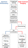 |
Fig. 1 Summary of the data reduction processing steps for aperture photometry and HCI. |
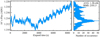 |
Fig. 2 Example of on-sky raw thermal background measurements obtained in the N’ band with the telescope pointing at an empty region of the sky and covering approximately 15 degrees of elevation change during the whole duration of the sequence. The left panel shows the flux integrated over a photometric aperture of 8 pixels in radius while the right panel shows the corresponding distribution. The complete figure and a more detailed analysis of the performances of the nulling data-reduction performances for the HOSTS survey can be found in Defrère et al. (2016). |
2.2 Datasets
β Leo dataset. For HCI, we used a dataset of β Leo, which is composed of two subdatasets. These two subdatasets were taken on the same night, UT 2015 February 8, along with their calibrators: HD 104979, HD 108381, and HD 109749. These sub-datasets are respectively composed of 8000 and 8800 frames with each a 60ms exposure time and an offset every 1000 frames (except for one group of 1800). The parallactic angle ranges of the two subdatasets are respectively from 41.11° to 45.02° and from 53.67° to 57.41°, and the smallest distance from the star center to the edge of the usable field of view corresponds to a distance of 0.6 arcsec.
Background-only dataset. For aperture photometry, the dataset was taken on UT 2015 November 11, and it is a background-only dataset composed of 24000 frames without any sky offsets. For this dataset, we recreated artificial groups using the 1000-frames-per-group model from the first dataset of β Leo. We thus alternated groups of “source” and “background” exposures as if a star was present.
2.3 General data reduction steps
The nodding sequence for our observations was composed of a top and a bottom position. We only kept the two left quadrants, as the right part of the detector was not used. We refer to the two left quadrants as the top and bottom images. The final size of these subframes is 123 × 123 pixels (pixel size: 17.9 milliarc-sec). We sort the images so the top and bottom images can be treated separately and then sort them per group. For β Leo, we had eight groups for each part of the two datasets. The groups of each part of the image alternate between ones with the star in them (source exposure) and those without the star (background exposures) due to the nodding between the groups. After this first step, we apply a bad pixel correction and a subtraction of the mean flux of each image from each individual pixel in that image (Offset Correction in Fig. 1).
2.3.1 Mean background subtraction
In the case of the mean background subtraction approach, we compute the mean of a sequence of dedicated background exposures and then subtract it from every on-source exposure. The high-contrast analysis used to search for circumstellar emission was then performed without further treatment of the background. The aperture photometry analysis was performed using a background annulus to estimate the background under the photometric aperture. The photometry in this annulus was then subtracted from the photometry in the region of interest. The resulting photometry was then used for further analysis. This approach is extensively described in Defrère et al. (2016).
2.3.2 PCA background subtraction
Pre-subtraction. Before performing a PCA background subtraction, it is useful to remove static spacial background structures using a pre-subtraction. This is beneficial because we have to use a mask to prevent over-subtraction from the star when computing the actual PCA for background subtraction. However, the mask strongly reduces the information available for principal component building. The pre-subtraction effectively reduces this loss of information and helps build an optimal background subtraction. We perform this pre-subtraction by subtracting a constant background frame from each individual image of a group. This image is derived from the background exposures only and without any mask. This step is similar to the mean background subtraction. In this case, we compute the PCA correction for the background exposures in the library, average the correction images obtained, and subtract this mean image from every on-source exposure.
Background subtraction. The PCA approach is commonly used in HCI to remove the stellar point spread function (PSF; Amara & Quanz 2012; Soummer et al. 2012; Amara et al. 2015). Here, we use it to better estimate and remove the sky background, similar to the approach used by Hunziker et al. (2018). We thus perform the PCA on background exposures. This determines the eigenvectors (or principal components) onto which the on-source images are projected. In order to avoid source over-subtraction, a mask on the star is introduced during this step (see below). With this technique, an optimal correction is computed for, and subtracted from, each on-source science image. This technique allows for an additional background removal compared to the classical subtraction for high-contrast analysis. In the case of aperture photometry, it replaces the background annulus used in the mean background subtraction. Indeed, PCA is capable of reconstructing the background at the position of the star, which constitutes a more sophisticated estimate than the background annulus.
Masking the star. A problem related to the PCA background subtraction is over-subtraction since the astronomical source (in our case a star) is present in the images we want to correct. To avoid over-subtraction, we thus mask the region of interest. We do not introduce a mask for mean background subtraction since the process never involves any information from the source exposure. The mask is necessary for PCA but limits the region of the source images that can be used for projecting the principal components. In addition, if PCA computes the principal components on unmasked data, it makes use of masked data to determine the PC weights used in the correction. However, in a perfect case with no astronomical source, the coefficients would also be determined using the unmasked data. One cannot guarantee that those coefficients obtained with the masked or unmasked data would be the same. The introduction of a mask therefore breaks the rule of orthogonality in PCA. This introduces an error in our correction and is a limiting factor on the PCA performance presented in this study.
Furthermore, the mask sizes range from 9 to 32 pixels in radius in our analysis, depending on the use case. While we can expect the smallest masks to have a very limited impact on the coefficients, the larger masks would introduce a larger error when applying the background subtraction. We thus expect our data with a mask of 9 pixels in radius to retrieve the coefficients with a better reliability, and thus to provide a correction of high quality compared to those with a mask of 32 pixels in radius. To check that the use of the mask does not significantly impair the PCA background subtraction, we applied our method to the background-only dataset. The results show that the correction was no longer optimal, even on the smallest mask size. However, the effect is generally relatively small and will not significantly impact the results presented in this study.
At the end of our background subtraction, we recombine both the top images and bottom images together to obtain a single dataset. This dataset is thus composed of the sub-frames selected in each original frame. This step is performed either just after background subtraction (aperture photometry) or after frame recentering the star (HCI).
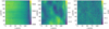 |
Fig. 3 Raw image (left), mean image of the dataset with a mean background subtraction (middle), and mean image of the dataset with a PCA background subtraction (right). For the PCA background subtraction, we used a mask of 32 pixels in radius in order to mask the central region where the star would be located if it was present in the data. |
2.4 Application to high-contrast imaging
For HCI, the β Leo datasets needed to be prepared for PSF subtraction. Thus, before recombining the datasets, all frames were re-centered so the star was at the center of each frame. The next step after the dataset recombination consisted of discarding the bad frames with a high null leak. This step is optional, as unfiltered datasets might provide better performances depending on the configuration. After this filtering step, in order to save computational time, we averaged the frames by groups of 100 images.
2.5 Application to aperture photometry
For aperture photometry, we used the background-only dataset. As we would have for a dataset containing an astronomical source, we used a mask during the PCA background subtraction and a background annulus for mean background subtraction. Since the source can be extended, we explored a range of circular photometric aperture sizes and matching mask and background annulus sizes. We explored two cases. In the first case, the photometric aperture matches the mask (i.e., the whole source flux is measured). This may be applied for both resolved and unresolved sources. For the second case, we still mask the entire (expected) source emission, but we use smaller apertures of varying sizes to determine the radial distribution of extended emission or a curve-of-growth aperture photometry. This case in particular applies to the HOSTS data of exozodiacal dust observations. For this last case, we used three different aperture sizes (8 and 13 pixels in radius and a conservative aperture that covers the whole emission), as was done during the HOSTS survey analysis (Ertel et al. 2020a; Defrère et al. 2021). However, to prevent the background correction from taking any extended emission into account, the mask have to cover the whole emission, even for smaller aperture sizes.
3 Results
An initial interesting result to display is a visual comparison of the image quality after mean or PCA background subtraction using a mask of 32 pixels in radius. In Fig. 3, we display a raw image along with the mean image of the background-only dataset when the background subtraction is performed with the mean method and the mean image of the same dataset when the background subtraction is performed with PCA. The structures that are present in the mean image of the dataset when the background subtraction is performed with the mean method almost completely disappear when the background subtraction is performed with PCA. One can also see that despite the use of a mask for the PCA background subtraction, the image is much cleaner even under the mask. This first result thus suggests that both the photometric measurement and the high contrast analysis benefit from the PCA background subtraction.
3.1 Contrast curves analysis: ADI, RDI, and without PSF subtraction
To estimate the improvement obtained with the PCA background subtraction, we compared the results obtained from the mean and the PCA background subtraction using the contrast curves obtained with three different processing techniques: ADI, RDI, and without PSF subtraction and simply proceeding to a derotation of the frames. For ADI and RDI, the PSF is subtracted with a full-frame PCA algorithm from the Vortex Image Processing (VIP; Gonzalez et al. 2017) library. It is important to distinguish between PCA background subtraction and full-frame PCA PSF subtraction. The PCA for background subtraction and the PCA for PSF subtraction do not use the same principal components number. Furthermore, the mask was only used for background subtraction and not for PSF subtraction.
After PSF removal, the contrast curves were computed using a 5-sigma threshold, and the throughput was obtained through fake companion injection. The fake companion injection was performed after background subtraction. Therefore, the throughput did not take into account possible subtraction of a potential companion during the background subtraction step. However, since the background correction was computed on off-source images, no signal from a potential companion was present in the library used to build the principal components. Hence, no planet signal was included in the principal components. Thus, self-subtraction could be ruled out. Projection of the PCs onto the science images may still result in an over-subtraction of the background around the potential companion if its presence can amplify some background signal in the PCs. However, this effect was expected to be negligible since the companion is typically very faint and the background dominates the projection of the small number of PCs. This conclusion is amplified by the fact that the companion does not stay at the same position with the parallactic angle range of the dataset. Given these considerations, we assumed that the companion would not be self-subtracted or over-subtracted during the background subtraction step.
For the ADI method, the PSF was removed using the full-frame PCA algorithm for PSF subtraction provided by the VIP library. The results are presented in the top panel of Fig. 4. The solid lines represent the best contrast curves obtained among the different pre-subtractions and principal component numbers used for the background subtraction. We used for both the solid and dashed lines and for both the mean and PCA background subtractions ten principal components for the PSF subtraction, as the convergence of the contrast curves was reached at this point for all the configurations compared in this figure. The dashed lines represent the best contrast curves obtained among the different aforementioned configurations but also among the different filtering levels. For the purpose of this analysis, we tested four filtering levels: 80%, 60%, 40% and 20% of the maximum photometry obtained in an 8-pixel aperture centered on the star. Thus, applying those filters resulted in the removal of all the frames for which the aperture photometry in an 8-pixel aperture centered on the star was above the threshold. For this particular case, the best filtering levels were reached at 60% for the mean background subtraction and 80% for the PCA background subtraction.
One can see in the top panel of Fig. 4 that PCA background subtraction provides the best results for both the filtered and non-filtered curves. For the optimally filtered case, the improvement obtained with the PCA can go up to 1.2, while for the unfiltered case, the improvement can go up to 1.7. It is, however, important to remember that these contrast curves are contrast limited for the whole range of angular separation due to the small field of view of our datasets. Thus, higher improvement factors are expected in background-limited regions.
As for the ADI case, we compared the contrast curves obtained through full-frame PCA PSF subtraction with RDI. For this analysis, we used the dataset of calibrator HD 108381, which is composed of 8000 frames of 60 ms exposure time. In the RDI case, both the scientific and calibrator datasets are background subtracted in the exact same way. We thus matched the calibrator observations that had been background subtracted with the same pre-subtraction, the same PC number for background subtraction, and the same filtering level to the corresponding scientific dataset. We present the results for this section in the middle panel of Fig. 4. In the case of the PCA background subtraction, the best results were obtained with ten principal components. The number of principal components for PSF subtraction are respectively eight and ten for the PCA background-subtracted cube and six and ten for the mean background-subtracted cube.
One can see in the middle panel of Fig. 4, that, as in the ADI case, the PCA background subtraction can bring an improvement to the contrast curves obtained with mean background subtraction. In the non-filtered case, we obtained an improvement factor of up to 1.2. However, we obtained improvement factors from 1.1 at large separations to 1.3 at small separations between the two optimally filtered curves. As in the ADI case, these contrast curves are contrast limited for the whole range of angular separations.
For the analysis without PSF subtraction, we only de-rotated the frames, and we formed the final image with the median frame of the de-rotated dataset. As there is no self-subtraction for this method, the throughput is everywhere at one. The main benefit of this method is enabling analysis of the effect of the background subtraction without the biases of the PSF subtraction. We present the results of this method in the bottom panel of Fig. 4. For the filtered (dashed) curves, a filtering of 20% for the mean background subtraction and for the PCA background subtraction has been applied.
Without PSF subtraction, the contrast strongly dominates since the residual starlight is not removed. This can be seen at close separations, where the contrast is the most problematic, and the PCA background subtraction does not improve the contrast curves. On the other hand, at a larger separation, where the impact of the contrast diminishes, the PCA background subtraction improves the contrast curves, as expected.
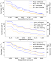 |
Fig. 4 Contrast curves obtained with ADI (top panel), RDI (middle panel) and without PSF subtraction (bottom panel) without (straight lines) and with optimal filtering (dashed lines) for mean background subtraction (blue) and PCA background subtraction (orange). A pre-subtraction with mean has been applied on the PCA background subtracted cube before we applied the 9-pixel mask on the star. |
3.2 Aperture photometry analysis
In this section, we display the results of our comparison of the mean and the PCA background subtracted datasets with aperture photometry on the empty dataset presented in Sect. 2.2. All apertures were placed on the center of the frame, where the star would be located if any were present.
3.2.1 General photometry
First, we discuss the case of general photometry, where the photometric aperture, background annulus (for classical mean background subtraction), and mask (for the PCA background subtraction) are optimized for the size of the observed astronomic source (e.g., star, galaxy). The mask therefore had the size of the source, and the background annulus inner radius was set to be exactly one pixel larger than the source extension. The outer radius of the background annulus was computed to match, as closely as possible, the mask and the annulus areas (no fractional pixels). For this case, we studied different possible source sizes ranging from 8 pixels to 32 pixels in radius. In the case of the mean background subtraction, the photometry was computed as the difference between the photometry obtained in the central aperture and the one obtained in the background annulus. Since their areas do not exactly match, we normalized these two quantities by the number of pixels contained in each. A pre-subtraction was applied before the PCA subtraction on both the scientific images and the background images. No mask and no pre-subtraction were applied for the mean background subtraction.
Figure 5 presents the results for three particular aperture sizes (8-pixel: optimized for point sources; 13-pixel: marginally extended sources; and 32-pixel: extended sources). Background residual structures appear in the curves and increase in magnitude for larger apertures. The RMS of our measurements degraded in a similar manner. Due to the large spikes, the degradation is particularly visible in the PCA curve for the largest aperture. In the case of mean background subtraction, the background annulus effectively flattens the spikes, and we instead obtained whole groups offset from zero. These structures in the photometry result from background structure residuals, and their variation, after the background subtraction was performed.
Next, we consider the mean retrieval of a source flux from the data. If no bias is present, the value should be consistent with zero within the statistical error σ of the data,  , with Nf being the number of frames in the group. This value is, respectively, from the smallest to largest aperture: 0.77, 1.75, and 4.13, for the mean background subtraction, and 0.77, 1.61, and 5.93 for the PCA background subtraction. This was not the case for any of our mean retrieval values, which indicated that there is a bias present for both the mean and PCA background subtraction. It is, however, interesting to note that in the case of PCA for the 8-pixels and 13-pixels apertures, if we exclude the easily identified outlier groups, the mean retrieval then respectively become 0.52 and 0.48, consistent with zero within the statistical error.
It is important to note that each of these long sequences, and their mean retrieval value, is only one random realization of the photometry and is thus affected by the quasi-statistical background bias and by large random errors. As the quasi-random effect of the background bias may result in a positive or negative offset with the statistical mode of its probability distribution at zero, a single measurement close to zero may be serendipitous and is not proof of a lack of background bias. As a consequence, the mean retrieval values of those longue sequences are not suitable for comparing the performance of the methods, as a worse performing method can get “lucky” and produce a more accurate value than a generally better-performing method due to random errors. It is thus not surprising that PCA produces a mean retrieval value that is further from zero than the result from the mean background subtraction in two of the three cases, and it is not a reliable indication that PCA performs worse than the mean background subtraction. To more reliably evaluate the performance of the two methods, we performed a statistical analysis on a per-group basis in, shown in Fig. 6.
In order to better compare the two methods, we computed, for each group of a thousand images, the mean retrieval value and its RMS. This comparison allowed us to both estimate the bias remaining in the data, if the points are significantly offset from zero, and the uncertainty of those values. The results are shown in Fig. 6. When using an 8-pixel or a 13-pixel aperture, some groups of images, when performing background subtraction with the mean method, are significantly offset from zero. An even more problematic characteristic is that the error bars of those measurements failed to account for their dispersion. On the other hand, with the PCA background subtraction, those groups are much closer to zero.
Figure 6 shows a clear improvement when using the PCA background subtraction instead of the classical mean background subtraction. Indeed the uncertainty of the HOSTS survey is dominated by the scattering of the measurement rather than by the measurement uncertainty themselves. It should be noted, however, that Fig. 6 presents the results for the 13-pixel aperture only. The 8-pixel aperture presents very similar results but for the scale at which the different measurements are scattered. For the 32-pixel aperture, the difference between the mean and the PCA background subtraction became less significant, in particular due to one extreme outlier. However, it is difficult with such plots to quantitatively estimate the improvement obtained with the PCA background subtraction. We thus decided to compare the ratio between the values obtained with the mean background subtraction and the PCA background subtraction instead in order to obtain improvement factors. We present those results in Fig. 7.
We computed improvement factors of the mean per group as the ratio between the absolute value of the mean from the classical background subtraction and the absolute value of the mean from the PCA background subtraction. For the RMS, we computed the improvement factor as the ratio between the RMS from the classical background subtraction and the RMS from the PCA background subtraction. The measurements from the individual groups were still randomly distributed around zero, and the individual improvement factors were thus distributed between zero and infinity with a mode below one (for a degradation) or above one (for an improvement). The results were thus still affected by a large statistical noise. We then computed the geometric mean of the improvement factors over all groups to suppress the statistical noise. We present those results in Fig. 7 for the mean retrieval (left panel) and the RMS (right panel). We rejected the outliers with a higher RMS, as could be done in a similar analysis of actual source photometry of a science target. However, to prevent rejecting too much exposure time, we limited the number of outliers to five (20% of data).
As can be seen in the left panel of Fig. 7 the mean retrieval benefits from a PCA background subtraction. We obtained, on average, an improvement factor between 1.3 and 2.4 for the mean retrieval. We did not see any clear tendency in the range of mask sizes except for the largest one, for which PCA background subtraction provides results of about the same quality as a standard mean background subtraction. In the right panel of Fig. 7, we observed that the RMS is much less impacted by the PCA background subtraction than the mean retrieval. This is because the RMS of the individual photometry measurements per image is dominated by background photon (Poisson) noise. The PCA method is powerful in removing subtle biases in the data that become significant when averaging a large number of frames or integrating for a long time, but it has little effect on the RMS of the photometry of individual frames, as those individual frames are dominated by noise. However, the smallest apertures and masks, which accumulate the least Poisson noise, still benefit (even if only slightly) from the PCA background subtraction. For the largest masks, however, we observed a slight degradation. The two plots in Fig. 7 show that even for a reasonably large aperture and mask, PCA can provide significant improvements and its effectiveness decreases only for large masks, as compared to the total size of the frame. Thus, in the case of a not-too-extended emission, the PCA background subtraction is much more effective than the mean background subtraction for aperture photometry.
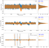 |
Fig. 5 Aperture photometry per frame with apertures of 8 (top panel), 13 (middle panel), and 32 (bottom panel) pixels in radius for the mean background subtraction (blue) and PCA (orange) background subtraction with a mask of 9, 13, and 32 pixels in radius. The gray boxes show the groups considered as outliers and not used for mean retrieval and RMS for both the mean and PCA background subtraction. The calibration factor for sensitivity is 1 ADU for 0.3 mJy. |
3.2.2 Varying mask sizes for a fixed aperture size
In this section, we explore the impact of varying the mask size for a given fixed aperture size. The mask is a significant constraining factor for the performance of the PCA method, as it limits the amount of information available for the PCA background subtraction. Scientifically, this is also an important study for the specific case of LBTI nulling interferometry for the HOSTS survey, as described in Sect. 2.5, where the mask needs to cover all plausible disk emission, while a smaller aperture can be used to optimize the expected signal-to-noise or to constrain the emission within a certain radius. More generally, one may want to adjust the mask size to the specific science case and data properties, just as one would do with the background annulus for classical background subtraction. The impact of varying the mask size thus needs to be understood.
As for the general case, we first compared the photometry across the whole sequence and then computed improvement factors based on a group-by-group analysis. In Fig. 8, we present the results of the latter for the 8-pixel photometric aperture and a range of mask and background annulus sizes optimized for the conservative apertures found for the HOSTS targets.
The left panel of Fig. 8 shows that the PCA background subtraction provides significantly better results than the mean background subtraction, with about a factor 1.7 to 2.5 improvement over the range of mask sizes. These improvement factors are mostly valid for the whole range of aperture, mask, and annu-lus sizes we probed. Even for the largest aperture, we did not observe any degradation on the mean retrieval. In the right panel of Fig. 8, we present the results for the RMS. One can see in this panel that PCA tends to improve the RMS for all aperture sizes. However, the improvements are quite small, and one can consider that the PCA method does not significantly impact the RMS compared to the mean method. The 13-pixel aperture is the optimal one for the HOSTS survey (Ertel et al. 2020a), and we present a detailed analysis for this aperture size together with two other mask sizes: 17 and 32 pixels, respectively the smallest and largest conservative apertures in the sample of the HOSTS survey.
The top panel of Fig. 9 shows a certain number of structures in both curves. The ones for the mean background subtraction are flatter due to the background annulus correction. As previously explained, we discarded the worst groups in terms of RMS for the computation of the mean retrieval and the RMS on the whole dataset. Outside of the group impacted by those structures, we observed that PCA provides a more stable photometry. The general mean retrieval in the first panel is only slightly better for PCA than with the mean method. For the second panel, it is even slightly degraded. This is due to the groups averaging themselves out better in the case with the mean background subtraction than in the case of the PCA background subtraction. However, this does not translate the real quality of the mean retrieval in the dataset. This is why we prefer the group-per-group analysis, which provides more measurements and thus a more precise estimate of the mean retrieval quality and the improvement brought by the PCA background subtraction. The group-per-group analysis over the range of conservative apertures is shown in Fig. 10.
The left panel of Fig. 10 shows, as in Fig. 8, that the PCA method is more effective than the mean background subtraction for the mean retrieval. Here, we obtained a factor of around two improvement over most of the range. In the right panel, for the RMS, we observed that PCA still performs slightly better than the mean background subtraction, with similar factors to the 8-pixel case.
The case with an aperture of 32 pixels in radius is similar to the general case, as we already showed in Sect. 3.2.1 and for which we have demonstrated that the mean retrieval remains almost the same as in the mean background subtraction case and the RMS is only slightly degraded. This largest aperture aside, in this second case, too, the PCA background subtraction provides significantly better results, with improvement factors ranging from 1.7 to 2.5 for most apertures and mask sizes.
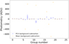 |
Fig. 6 Comparison of the mean retrieval ADU values per group of 1000 images and their respective errors bars with an aperture of 13 pixels in radius, for mean background subtraction (orange points) and PCA background subtraction with a mask of 32 pixels in radius (blue points). |
3.2.3 Varying aperture size for a fixed mask size
It is also interesting to investigate the effect of a fixed large mask size and varying size of the photometric apertures. The different sizes of aperture can be used to determine the radial distribution of extended emission (e.g., exozodiacal dust in HOSTS data and extended galaxies) or for curve-of-growth photometry of point sources. Here we use the case of β Leo from the HOSTS survey as a proxy and present the results for the conservative aperture of this star. The mask radius was thus set to 32 pixels and the inner radius of the background annulus to 33 pixels. These results are presented in Fig. 11.
An interesting feature can be seen in the left panel of Fig. 11. With a fixed mask size, we still observed a degradation of the improvement factors toward a large aperture. The PCA background subtraction is thus more sensitive to the increase of the aperture size than the mean background subtraction. In terms of improvement factors, we obtained a significant improvement over most of the range of aperture sizes. If we exclude the last aperture size (32 pixels in radius), we obtain improvement factors ranging from 1.4 to 3.2. This case shows that even with a really large mask, the small apertures benefit strongly from the PCA background subtraction. Additionally we did not observe any degradation when using the PCA background subtraction instead of the mean background subtraction, over the whole range of aperture sizes in this case.
As can be seen in the right panel of Fig. 11, the RMS does not significantly benefit from the PCA background subtraction with such a large mask. However, we did not observe any significant degradation either.
3.3 Ring apertures
In a recent effort to improve the null measurement of the HOSTS survey, we have begun to use annulus photometry instead of filled circular apertures. The advantage of this is that the ringlike photometric aperture can be placed at the region where the extended dust emission is expected while ignoring a significant fraction of the residual star light. Furthermore, the use of different ring radii may allow one to characterize the radial distribution of the dust for the more extended systems (Faramaz et al., in prep). In order to better estimate the real improvement brought by PCA with this new geometry for null measurement, we also performed annulus photometry instead of circular aperture photometry. We obtained similar improvement factors for both the mean retrieval and RMS. However, for larger apertures, we observed slightly better results. In particular, we did not observe any degradation when using the annulus apertures instead of circular apertures. Thus, we expect the PCA background subtraction to improve the results of the null measurements with an annular aperture, at least as much as it would for a circular aperture.
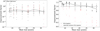 |
Fig. 7 Improvements factors when using PCA background subtraction instead of mean background subtraction for mean retrieval (left panel) and RMS (right panel). Each point represents the ratio of the value obtained for PCA background subtraction and mean background subtraction. The background annulus inner radius is always one pixel larger than the mask radius. For each dataset, with its given mask and annulus size, we rejected up to 5 outliers which are here represented in red. These outliers are determined with respect to their RMS. The solid line represents the geometric mean of the improvement factors of individual nods, without the outliers. |
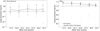 |
Fig. 8 Same as Fig. 7 but with a fixed aperture size (8 pixels) and varying size of the PCA mask and background annulus. |
4 Discussion
4.1 Limitations and path forward
Figures 5 and 9 show that the PCA background subtraction can fail for particular groups of images with large spikes in the frame-per-frame photometry. We investigated potential sources for these failures, and we have shown that the groups with the strongest spikes can be easily identified by their increased RMS of the photometry. This provided an option to deal with them by simply ignoring the data in those spikes. However, a solution that would retain all data is preferable.
To investigate the origin of these failures, we first applied a background annulus to the aperture photometry after PCA background subtraction. This successfully suppressed the spikes similar to the case of classical mean background subtraction.
This is shown in Fig. 12. We concluded that the spikes are not introduced by the PCA but are rather not as well suppressed as by the background annulus. We then explored different sources of the spikes in the images, including (1) a compact, bright structure in the aperture and under the mask that cannot be corrected by the PCA; (2) a compact, bright structure located outside the aperture that is brought into the photometry of the aperture due to the correction; (3) a largely extended structure, both outside and in the aperture, whose brightness rapidly varies; (4) a rapid overall brightness variation of the background.
From these hypotheses we started to rule out the different options, particularly those with a compact structure. Since the large spikes appear both for the PCA and the mean background subtraction when not using a background annulus, hypothesis (2) is very unlikely. A mean background subtraction would not bring the photometry of this small bright structure into the photometry of the aperture. Thus, those spikes would not be observed in the photometry with the mean method when no background annulus is used.
In addition, the use of the background annulus for both the mean and PCA background subtraction flattens the spikes, which then only appear as small offsets. This behavior also rules out hypothesis (1) since a small bright spike in the photometric aperture would not be flattened by an annulus of background that does not contain this structure.
In addition, we tried to change the location of the aperture in the image. With this change of position, some spikes appeared for different groups, and some that were present with the centered aperture disappeared. However, for the group presenting the strongest spike (from frame 10000 to 11000) in Figs. 5 and 9, the spike remains at whichever location we placed the photometric aperture. As a small bright structure would not appear in all the apertures at different locations on the image, this rules out the possibilities described in hypotheses (1) and (2) of a small structure.
We thus concluded that the reason for those failures must be related to hypotheses (3) or (4), with a brightness variation of an extended emission which would be too significant or too fast for PCA to correct for it. We also found that, even for the smallest aperture (8 pixels in radius), this structure appears when using a larger mask.
The simplest solution to overcome this problem would thus be to limit the size of the mask, but this would be a very strong constraint on the possible ways to apply the method. Another possibility is to use a background annulus with the aperture photometry in addition to the PCA background subtraction. This, however, defeats the purpose of the PCA, as the background annulus adds photon noise and at least some of the background bias back into the data. The results shown in Fig. 12 use an optimal configuration in which the inner radius of the background annulus is one pixel larger than the photometric aperture radius. In cases such as those discussed in Sect. 3.2.3 in which the mask and the inner radius of the background annulus are larger than the photometric aperture, this technique does not work effectively, and the spikes remain.
The optimal solution would be to address the rapid brightness variation of the overall image or of the extended structure over time. For this purpose, we will develop a temporal PCA approach which would significantly reduce the background brightness variation over time. This temporal PCA would thus builds its principal components on the variation of individual pixels through time. Since the large-scale variations of the background correlate for a large number of pixels that are located close to each other in the image, the temporal PCA will identifies these variations as dominant features in the data that can then be removed. We also expect this procedure to reduce the differences between the background exposures and the source exposures (as the variation of pixels over time will be reduce for both), thus allowing for a better correction than with the spatial PCA alone.
Since the actual source flux variation in the image is not used afterward in the case of regular photometry, it may not have to be masked during the temporal PCA step. For nulling interferometry, the instrumental null depth does, however, vary over time, and this variation is used for the statistical analysis of the data (null self-calibration; Defrère et al. 2016). While the PCA may potentially provide an alternative way to analyze the null variation that could be explored, masking the star will still be required if the null variation is to be preserved for further analysis. The dust emission region may, however, not need to be masked, similar to the case of regular photometry. This provides an opportunity to eliminate the mask, or at least reduce its size, which is a major performance limitation of the PCA method.
As a first estimate of the possible improvement, we used the background annulus already used for mean background subtraction. This is shown in Fig. 12. One can see in this figure that the spikes disappear and the RMS is reduced by about a factor of three. This estimate shows how much we can improve our results by completely removing the spikes. It is possible that the temporal PCA correction performs slightly worse, as the small photometric variations that remain would degrade the RMS but nonetheless still allow those groups of images to be used and improve the mean retrieval. On the other hand, the temporal PCA correction should not only affect the groups of images with the spikes in photometry but also reduce the RMS in the less extreme groups of images. In a group-per-group analysis to estimate performances with and without a background annulus, we observed that the mean retrieval is significantly degraded on most of the groups with the use of the annulus. However, we do not expect such an effect with the temporal PCA correction. Indeed, the bias comes from the spatial difference between the aperture location and the background annulus location. With the use of the temporal PCA correction, only the principal components would be computed at a different location, while the projection would be performed on the aperture location, thus limiting this effect.
As shown in the case of aperture photometry, some structures are not perfectly removed by the spatial PCA background subtraction. These likely large-scale, time-variable structures causing the spikes on the photometry sequence will also affect the HCI case, where they may be limited to the achieved contrast or possibly result in a spurious detection. Further investigation of the benefits of temporal PCA in HCI datasets is likely of merit as well.
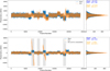 |
Fig. 9 Similar to Fig. 5 but with a fixed aperture size of 13 pixels in radius and a mask radii of 17 (top panel) and 32 pixels (bottom panel). The calibration factor for sensitivity is 1 ADU for 0.3 mJy. |
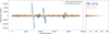 |
Fig. 12 Similar to Fig. 1 but comparing PCA background subtraction with (orange curve) and without (blue curve) background annulus. The aperture and mask size are 32 pixels in radius, and the inner radius for the background annulus is 33 pixels. The calibration factor for sensitivity is 1 ADU for 0.3 mJy. |
4.2 Application to HOSTS and nulling data
The HOSTS survey was able to put an already much stronger constraint than previous missions on the median zodi level around nearby stars. This median level is of primary importance for future direct imaging missions for exoplanets since a large amount of zodiacal dust in a system can easily outshine and hide an Earth-like planet. Even if the HOSTS survey has already demonstrated that the median zodi level would not definitively prevent a direct-imaging mission to image an Earthlike planet, the sensitivity of its measurement would need to be improved by a factor of two in order to address the feasibility of direct-imaging missions currently under development, such as the Habitable Worlds Observatory (HWO).
In our analysis, this sensitivity improvement would translate into an improvement of the mean flux retrieval. Thus, it is interesting to see that in all cases except for the largest aperture (32 pixels in radius), the improvement factors on the mean retrieval are about two. From the conservative aperture radii used in Ertel et al. (2020a), only six stars of 38 have conservative apertures equal or above 32 pixels in radius. We thus expected this factor of two to translate directly into nulling measurements over all three apertures for most stars. In future work, we intend to apply this new method to the whole HOSTS survey target sample and reanalyze the data with the new PCA background subtraction. From this factor of two to three improvement on the mean retrieval, we expect to both put stronger constraints on the already detected exozodis and increase the number of detections among the HOSTS target sample. Furthermore, we intend to perfect this method with the introduction of the temporal correction described in Sect. 4.1, in addition to the spatial correction described in this work. This new analysis of the HOSTS survey will strongly benefit future direct imaging missions.
We also believe that developing similar PCA-based approaches for single-mode fiber-fed nulling instruments, such as the Nulling Observations of exoplaneTs and dusT instrument (NOTT; Defrère et al. 2018, 2022), and missions such as the Large Interferometer For Exoplanets (LIFE; Quanz et al. 2022) would be strongly beneficial. A PCA-based approaches would, indeed, push their sensitivity and improve their science return by improving their detection limits and reducing the time needed for individual observations.
4.3 General applications
The results shown in this article are valid for the nulling-interferometric data of the HOSTS survey. However, this method can be applied to a much wider range of data types and observations. In this section, we discuss how the improvement obtained with PCA might change in function of different data parameters, such as the predominance of background bias relative to its RMS in the data, or observational parameters, such as the nodding frequency or the time needed for an offset.
The sensitivity is limited by several sources of noise. Here, we estimate the contribution of different noise sources for both the mean and PCA background subtraction. In particular we show in Fig. 13 the effects of the photon noise, the ELFN noise (RMS), and the bias with respect to the integration time.
As can be seen in Fig. 13, the PCA background subtraction has very little effect on the RMS. However, it significantly improves the bias left after the background subtraction. With sufficient integration time, this bias improvement directly translates into a sensitivity improvement. For both of the datasets used in this article, the integration time is long enough such that the sensitivity is limited by the bias for both the mean and PCA. Similarly, all the datasets from the HOSTS survey are in the regime limited by the bias. Thus, it is reasonable to expect similar improvement factors. With the temporal PCA additional correction we discussed in the previous subsection, we expect to push the RMS closer to the photon noise limit. Such an improvement would prevent the imposed limitation of the RMS for shorter integration times.
Another important parameter for the background subtraction is the nodding frequency. The shorter the frequency, the less the background will change between background exposures and source exposures. However, in the case of PCA, having a larger library to build the principal components can be beneficial. In Fig. 14, we show the effect of the nodding frequency on the limiting uncertainty.
As can be seen in Fig. 14, for a short-enough nodding frequency, we remain within reasonable limits on the uncertainty. However, with longer periods, the uncertainty increase rapidly. An interesting result shown in this figure is that the PCA background subtraction allows for the use of a longer nodding frequency compared to the mean background subtraction. The datasets used in this article have a nodding frequency of 45s. In this configuration, both the mean and PCA background subtraction remain within reasonable uncertainty limits. However, for the rest of the HOSTS survey, the nodding frequency was about 90−120 s. With this new configuration, we observed that using the PCA background subtraction becomes more advantageous. Thus, in general, using the PCA background subtraction allows one to use longer nodding periods.
In the case of the background dataset used for aperture photometry, we simulated groups of 1000 frames. However, since this dataset was taken with no sky offset, the simulated offset was instantaneous. To simulate a more realistic dataset, we thus tried different gap times during which a real offset would happen. We considered gap times from 0 to 140s for both the mean and PCA background subtraction. As expected, we found that the quality of the background subtraction decreases with an increasing gap time. However, this degradation is very similar for both background subtractions. We thus expect this parameter to have little to no impact on the improvement factors obtained with the PCA background subtraction.
Finally the improvement achieved by the PCA background subtraction would depend on the wavelength. Hunziker et al. (2018) applied a similar method in the L and M band, which benefits from a lower thermal background than in the N band, and found a smaller impact of the PCA background subtraction. Analogous studies should be performed with longer wavelengths to determine the real impact of such a method on a longer waveband.
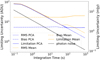 |
Fig. 13 Main sensitivity limitation in background-subtracted data, with an aperture of 13 pixels in radius for mean background subtraction (orange) and PCA background subtraction (blue). The photon noise is indicated in black. |
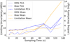 |
Fig. 14 Sensitivity limit as a function of time for background subtracted data. |
5 Summary and conclusions
This study shows that PCA thermal background subtraction can achieve significant improvement over mean background subtraction for both aperture photometry and HCI in the mid-infrared (N-band). For the latter, we have demonstrated that a PCA background subtraction can improve the reachable contrast by a factor 1.2 to 1.7. We have shown that this improvement is significant for both the very commonly used ADI and RDI PSF subtraction techniques, but without any PSF removal, the contrast dominates too much to observe any significant improvement.
For aperture photometry, we have shown in particular that without degrading the photometric precision, we can reach an improvement factor of 1.4 to 3.2 on the accuracy of the mean retrieval. Imperfect thermal background subtraction has been shown to be a major sensitivity limitation of the HOSTS survey (Defrère et al. 2016). This limitation is mainly due to the bias on the individual calibrated null measurements rather than their error bars. With a factor 1.7 to 2.5 improvement on the accuracy of the mean retrieval over most of the range of apertures, we expected an improvement of a factor of about two for those biases and thus on the sensitivity. Further improvement of the nulling mode depends on the brightness of the star and requires further investigation.
The approach presented in this work can be applied to a wide variety of existing datasets and future observations since it only requires background observations that are regularly interleaved with the science observations (e.g., through nodding). All existing datasets with these characteristics would be suitable for this method. We strongly expect suitable existing datasets to benefit from this PCA background-subtraction approach with similar improvement factors. Similarly, future datasets with these characteristics, such as data taken by JWST, large ground-based telescopes, and future ELTs, would also strongly benefit from this approach. An improvement factor of up to three in sensitivity in thermal infrared observations will make them up to nine times less time-consuming and hence greatly improve the science return of observatories collecting these data.
Acknowledgements
H.R., S.E., and V.F. are supported by the National Aeronautics and Space Administration through the Exoplanet Research Program (Grant No. 80NSSC21K0394). D.D. acknowledges the support from the European Research Council (ERC) under the European Union’s Horizon 2020 research and innovation program (grant agreement CoG–866070).
References
- Amara, A., & Quanz, S. P. 2012, MNRAS, 427, 948 [Google Scholar]
- Amara, A., Quanz, S. P., & Akeret, J. 2015, Astron. Comput., 10, 107 [NASA ADS] [CrossRef] [Google Scholar]
- Defrère, D., Hinz, P. M., Mennesson, B., et al. 2016, ApJ, 824, 66 [CrossRef] [Google Scholar]
- Defrère, D., Absil, O., Berger, J. P., et al. 2018, Exp. Astron., 46, 475 [CrossRef] [Google Scholar]
- Defrère, D., Hinz, P. M., Kennedy, G. M., et al. 2021, AJ, 161, 186 [CrossRef] [Google Scholar]
- Defrère, D., Bigioli, A., Dandumont, C., et al. 2022, SPIE Conf. Ser., 12183, 121830H [Google Scholar]
- Ertel, S., Defrère, D., Hinz, P., et al. 2018, AJ, 155, 194 [Google Scholar]
- Ertel, S., Defrère, D., Hinz, P., et al. 2020a, AJ, 159, 177 [Google Scholar]
- Ertel, S., Hinz, P. M., Stone, J. M., et al. 2020b, SPIE Conf. Ser., 11446, 1144607 [Google Scholar]
- European Southern Observatory 1998, The VLT White Book (Garching near Munich: European Southern Observatory (ESO)) [Google Scholar]
- Fanson, J., Bernstein, R., Ashby, D., et al. 2022, SPIE Conf. Ser., 12182, 121821C [NASA ADS] [Google Scholar]
- Gardner, J. P., Mather, J. C., Clampin, M., et al. 2006, Space Sci. Rev., 123, 485 [Google Scholar]
- Gilmozzi, R., & Spyromilio, J. 2007, The Messenger, 127, 11 [Google Scholar]
- Gonzalez, C. A. G., Wertz, O., Absil, O., et al. 2017, Am. Astron. Soc., 154, 7 [Google Scholar]
- Hill, J. M., Green, R. F., & Slagle, J. H. 2006, SPIE Conf. Ser., 6267, 62670Y [NASA ADS] [Google Scholar]
- Hinz, P. M., Defrère, D., Skemer, A., et al. 2016, Proc. SPIE, 9907, 990704 [NASA ADS] [CrossRef] [Google Scholar]
- Hoffmann, W. F., Hinz, P. M., Defrère, D., et al. 2014, SPIE Conf. Ser., 9147, 91471O [NASA ADS] [Google Scholar]
- Hunziker, S., Quanz, S. P., Amara, A., & Meyer, M. R. 2018, A&A, 611, A23 [NASA ADS] [CrossRef] [EDP Sciences] [Google Scholar]
- Kasper, M., Arsenault, R., Käufl, H. U., et al. 2017, The Messenger, 169, 16 [NASA ADS] [Google Scholar]
- Quanz, S. P., Ottiger, M., Fontanet, E., et al. 2022, A&A, 664, A21 [NASA ADS] [CrossRef] [EDP Sciences] [Google Scholar]
- Riccardi, A., Xompero, M., Briguglio, R., et al. 2010, SPIE Conf. Ser., 7736, 77362C [Google Scholar]
- Sanders, G. H. 2013, J. Astrophys. Astron., 34, 81 [NASA ADS] [CrossRef] [Google Scholar]
- Soummer, R., Pueyo, L., & Larkin, J. 2012, ApJ, 755, L28 [Google Scholar]
- Werber, Z., Wagner, K., & Apai, D. 2023, AJ, 165, 133 [NASA ADS] [CrossRef] [Google Scholar]
- Werner, M. W., Roellig, T. L., Low, F. J., et al. 2004, ApJS, 154, 1 [NASA ADS] [CrossRef] [Google Scholar]
All Figures
|
Fig. 1 Summary of the data reduction processing steps for aperture photometry and HCI. |
| In the text | |
|
Fig. 2 Example of on-sky raw thermal background measurements obtained in the N’ band with the telescope pointing at an empty region of the sky and covering approximately 15 degrees of elevation change during the whole duration of the sequence. The left panel shows the flux integrated over a photometric aperture of 8 pixels in radius while the right panel shows the corresponding distribution. The complete figure and a more detailed analysis of the performances of the nulling data-reduction performances for the HOSTS survey can be found in Defrère et al. (2016). |
| In the text | |
|
Fig. 3 Raw image (left), mean image of the dataset with a mean background subtraction (middle), and mean image of the dataset with a PCA background subtraction (right). For the PCA background subtraction, we used a mask of 32 pixels in radius in order to mask the central region where the star would be located if it was present in the data. |
| In the text | |
|
Fig. 4 Contrast curves obtained with ADI (top panel), RDI (middle panel) and without PSF subtraction (bottom panel) without (straight lines) and with optimal filtering (dashed lines) for mean background subtraction (blue) and PCA background subtraction (orange). A pre-subtraction with mean has been applied on the PCA background subtracted cube before we applied the 9-pixel mask on the star. |
| In the text | |
|
Fig. 5 Aperture photometry per frame with apertures of 8 (top panel), 13 (middle panel), and 32 (bottom panel) pixels in radius for the mean background subtraction (blue) and PCA (orange) background subtraction with a mask of 9, 13, and 32 pixels in radius. The gray boxes show the groups considered as outliers and not used for mean retrieval and RMS for both the mean and PCA background subtraction. The calibration factor for sensitivity is 1 ADU for 0.3 mJy. |
| In the text | |
|
Fig. 6 Comparison of the mean retrieval ADU values per group of 1000 images and their respective errors bars with an aperture of 13 pixels in radius, for mean background subtraction (orange points) and PCA background subtraction with a mask of 32 pixels in radius (blue points). |
| In the text | |
|
Fig. 7 Improvements factors when using PCA background subtraction instead of mean background subtraction for mean retrieval (left panel) and RMS (right panel). Each point represents the ratio of the value obtained for PCA background subtraction and mean background subtraction. The background annulus inner radius is always one pixel larger than the mask radius. For each dataset, with its given mask and annulus size, we rejected up to 5 outliers which are here represented in red. These outliers are determined with respect to their RMS. The solid line represents the geometric mean of the improvement factors of individual nods, without the outliers. |
| In the text | |
|
Fig. 8 Same as Fig. 7 but with a fixed aperture size (8 pixels) and varying size of the PCA mask and background annulus. |
| In the text | |
|
Fig. 9 Similar to Fig. 5 but with a fixed aperture size of 13 pixels in radius and a mask radii of 17 (top panel) and 32 pixels (bottom panel). The calibration factor for sensitivity is 1 ADU for 0.3 mJy. |
| In the text | |
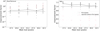 |
Fig. 10 Similar to Fig. 8 but for a 13-pixel aperture. |
| In the text | |
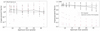 |
Fig. 11 Similar to Fig. 7 but with a fixed mask radius of 32 pixels and varying aperture sizes. |
| In the text | |
|
Fig. 12 Similar to Fig. 1 but comparing PCA background subtraction with (orange curve) and without (blue curve) background annulus. The aperture and mask size are 32 pixels in radius, and the inner radius for the background annulus is 33 pixels. The calibration factor for sensitivity is 1 ADU for 0.3 mJy. |
| In the text | |
|
Fig. 13 Main sensitivity limitation in background-subtracted data, with an aperture of 13 pixels in radius for mean background subtraction (orange) and PCA background subtraction (blue). The photon noise is indicated in black. |
| In the text | |
|
Fig. 14 Sensitivity limit as a function of time for background subtracted data. |
| In the text | |
Current usage metrics show cumulative count of Article Views (full-text article views including HTML views, PDF and ePub downloads, according to the available data) and Abstracts Views on Vision4Press platform.
Data correspond to usage on the plateform after 2015. The current usage metrics is available 48-96 hours after online publication and is updated daily on week days.
Initial download of the metrics may take a while.