| Issue |
A&A
Volume 687, July 2024
|
|
|---|---|---|
| Article Number | A11 | |
| Number of page(s) | 14 | |
| Section | Numerical methods and codes | |
| DOI | https://doi.org/10.1051/0004-6361/202245620 | |
| Published online | 25 June 2024 | |
Beyond Circular Eclipsers (BeyonCE) light curve modelling
I. Shallot Explorer
Leiden Observatory, University of Leiden,
PO Box 9513,
2300 RA
Leiden, The Netherlands
e-mail: dmvandam@strw.leidenuniv.nl; kenworthy@strw.leidenuniv.nl
Received:
5
December
2022
Accepted:
5
April
2024
Context. Time series photometry offers astronomers the tools to study time-dependent astrophysical phenomena, from stellar activity to fast radio bursts and exoplanet transits. Transit events, in particular, are focussed primarily on planetary transits and eclipsing binaries with eclipse geometries that can be parameterised with a few variables. However, more complex light curves caused by the substructure within the transiting object would require a customised analysis code.
Aims. We present Beyond Circular Eclipsers (BeyonCE), which reduces the parameter space encompassed by the transit of circumsec-ondary disc (CSD) systems with azimuthally symmetric, non-uniform optical-depth profiles. By rejecting disc geometries that are not able to reproduce the measured gradients within their light curves, we can constrain the size and orientation of discs with a complex sub-structure.
Methods. We mapped out all the possible geometries of a disc and calculated the gradients for rings crossing the star. We then rejected those configurations where the measured gradient of the light curve is greater than the theoretical gradient from the given disc orientation.
Results. We present the fitting code BeyonCE and demonstrate its effectiveness in considerably reducing the parameter space of discs that contain an azimuthally symmetric structure. We used the code to analyse the light curves seen towards J1407 and PDS 110, attributed to CSD transits.
Key words: methods: numerical / eclipses / planets and satellites: rings
© The Authors 2024
 Open Access article, published by EDP Sciences, under the terms of the Creative Commons Attribution License (https://creativecommons.org/licenses/by/4.0), which permits unrestricted use, distribution, and reproduction in any medium, provided the original work is properly cited.
This article is published in open access under the Subscribe to Open model. Subscribe to A&A to support open access publication.
1 Introduction
Times series photometry has led to tremendous physical insights into astrophysical processes thanks to the ability to measure the intensity of a star with high cadence, precision, and accuracy over long temporal baselines. A myriad of data highlighting the vast range of stellar variability exhibited on all timescales has been made possible via several ground-based surveys, such as All Sky Automated Survey for Super-Novae (ASAS-SN; Shappee et al. 2014; Kochanek et al. 2017), Asteroid Terrestrial-impact Last Alert System (ATLAS; Tonry et al. 2018; Heinze et al. 2018), Super Wide-Angle Search for Planets (SWASP; Pollacco et al. 2006). Valuable data have also come from a number of space-based surveys, such as the Kepler mission (Borucki et al. 2010), which was extended to the K2 mission (Howell et al. 2014) and Transiting Exoplanet Survey Satellite (TESS; Ricker et al. 2015).
It has been reported that intrinsic stellar variability may be caused by high-amplitude optical variability of young stars (Joy 1945), rotational starspot modulation (Rodono et al. 1986; Olah et al. 1997), or asteroseismology (Handler 2013). Other sources of variability include interactions of the star with other objects or dust orbiting the star. ‘Dipper’ stars are a class whose stellar variability arises due to occultations by dust in the inner boundaries of circumstellar discs, which produce transits with depths of up to 50% (Alencar et al. 2010; Cody et al. 2014; Cody & Hillenbrand 2018). Ansdell et al. (2019) found that this variability requires the misalignment of the inner protoplanetary disc compared to the circumstellar disc. Another interesting source of variability is stellar occultations due to the transit of a body.
The transiting bodies could be: (1) planets (Fischer et al. 2014) characterised by short symmetrical dips with regular periods and fixed transit depths, (2) exo-comets, which are characterised by a saw-tooth eclipse as seen in Fig. 2 of Zieba et al. (2019); or (3) disintegrating planets characterised by regular periods, but varying transit depths due to loss of planetary material (Rappaport 2012; Lieshout & Rappaport 2018; Ridden-Harper et al. 2018). (4) An additional source of variability is the transit of tilted and inclined circumplanetary discs. Due to projection effects, these create elliptical occulters that generate asymmetric eclipse profiles in the resultant light curve.
There are two leading theories for gas giant formation. The first is gravitational instability (Kratter & Lodato 2016), when gravitational instabilities in the protoplanetary disc result in gas and dust collapse under its own gravity and eventually forms a planet with a similar metallicity to the protostellar cloud (the top-down formation). The second is core-accretion (Helled et al. 2014), where a core grows to a sufficiently large mass that it starts to pull gas from its surroundings onto itself (bottom-up). As circumstellar material is transferred into the Hill sphere of the forming protoplanet, the material forms an accretion disc that depletes material on that orbital radius from the star and can produce cavities that are observable in the optical and sub-millimetre wavelengths (Benisty et al. 2021); it may also form spiral arms at this point. In both cases of planet formation, a disc forms around the protoplanet, which, in turn, can potentially support moon formation (Teachey et al. 2018). Expectations suggest that these circumplanetary discs are large (of the order of AU) and should be clearly visible as transits in time-series photometry (Mamajek et al. 2012). Problems arise in the fact that planet-searching algorithms were not designed to identify such transits, as the eclipses would be too long, deep, and complex to be identified an an exoplanet transit. The number of parameters to describe the geometry of the transit is already quite large, given the fact that there are many astrophysical effects that need to be taken into consideration. There are currently several prime candidates for occulting circumplanetary discs: V928 Tau (van Dam et al. 2019), EPIC 204376071 (Rappaport et al. 2019), and EPIC 220208795 (van der Kamp et al. 2022). Some candidates exhibit much more complex sub-structure reminiscent of rings: 1SWASP J140745.93–394542.6J1407 (J1407, Kenworthy & Mamajek 2015) and PDS 110 (Osborn et al. 2017, 2019).
The Shallot Explorer is a module of the Beyond Circular Eclipsers (BeyonCE) package that can limit the extended parameter space of circumplanetary ring systems (Sect. 2), based on measurements taken from the light curve (Sect. 3). The Shallot Explorer is described in detail in Sect. 4, with the results of simulations described in Sect. 5 and validations of the parameter space on real data discussed in Sect. 6. Finally, Sect. 7 presents the discussion and conclusions.
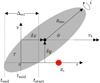 |
Fig. 1 Disc parameters. Symbols are the same as in Table 1. Scale factors in the table are not included here as they are contained by Rdisc and i. |
Disc parameters.
2 Circumsecondary disc parameters
The parameters that define the geometry and orientation of the disc with respect to our line of sight are shown in Fig. 1 and listed in Table 1.
The disc is assumed to be circular, with a scale height (hdisc) considerably smaller than the radius of the star (R*) and the radius of the disc (Rdisc):

The disc is inclined to our line of sight by angle, i, where i = 0° is a face-on disc and i = 90° is an edge-on disc. This presents an elliptical cross section with semi-major axis of Rdisc and semi-minor axis of Rdisc cos i. The path of the disc in front of the star with radius of R* is defined as going in a straight line moving with a constant projected transverse velocity of υt. The angle between the path of the disc and the on-sky projected semi-major axis of the disc is defined as the tilt, ϕ. The perpendicular distance (w.r.t. the path of the disc) from the centre of the projected disc to the centre of the star is the impact parameter δy. Since the diameter of the star typically contains the largest relative uncertainty of all the physical components in the system, we chose to represent size of the stellar disc in units of time, usually days, where the physical size of the disc can be converted from time to distance by multiplying by υt.
The inclination, tilt, and radius of the disc define the geometry of the disc projected onto the plane of the sky. The light curve is characterised by the first ingress of the star at tstart and egress at tend. Exactly between these two values lies tmid, such that tmid – tstart = tend – tmid. Thus, the disc geometry combined with the impact parameter ôy defines the chord that the disc makes as it moves in front of the star. We limit the range of δy to be a positive value and the 0 ≤ ϕ ≤ 180 because there is a geometric degeneracy in the transit geometry. The transit geometry for an occulter with δy = y0 and ϕ = ϕ0 is the same as an occulter with δy = −y0 and ϕ = 180 – ϕ0.
We define a Cartesian coordinate system in the plane of the sky, with the origin centred at the midpoint of the eclipse, tmid = 0. The centre of the projected disc is at (δx, δy) as shown in Fig. 1.
Though there are many effects that alter the evolution of a light curve during an eclipse such as intrinsic stellar variability, forward scattering of light from the star on the circumplane-tary disc (see van Kooten et al. 2020; Budaj 2013), magnetic interactions between the circumstellar material and the host star (Kennedy et al. 2017); we consider the limiting case where a star can be modelled as a sphere, with radius, R*. We allow for the model of the star to include limb-darkening as described by the linear limb-darkening law, which is parameterised by the limb-darkening parameter, u, as described in Eq. (1). It is expressed as

We note that µ = cos γ, where γ is the angle between the line of sight and the emergent intensity and I(1) is the specific intensity at the centre of the stellar disc.
The occulter itself can be separated into various parameters. Starting with the physical objects, there is the anchor body itself, which we assume to be a fully opaque (T = 0) spherical body, with radius, Rp. This is supplemented by a larger disc centered on the body, which has a radius of Rdisc. This disc can have an intricate radial evolution of optical depth (this includes gaps, i.e. rings). This is modelled by separating the disc into any number of rings with an inner radius, Rx,in, an outer radius, Rx,out, and a ring transmission, Tx, that varies as a function of radial distance from the central body. The final parameter for the system is the centroid shift, δx, which is necessary to define the centre of the occulter with respect to the centre of the star.
The model simplifications are reiterated here. First, the stellar limb is assumed to be spherical, the star quiescent with no significant star spots on its disc, and with a limb-darkening profile that can be described by a linear limb-darkening law (Eq. (1)). The disc is assumed to be azimuthally symmetric about the anchor body both in geometry and transmission. This means that we assume that the transmission profile is one dimensional (1D), T = T(R), and that there are no disc misalignments (i ≠ i(R) and ϕ ≠ ϕ(R)). Finally, we assume a constant velocity and impact parameter for the duration of the eclipse (i.e. the path of the occulter as it transits the star is straight). This assumption is a consequence of the Rdisc >> R* and is justified in Appendix A.
3 Light curve measurements
A light curve provides information about the star and the transiting object. We can determine the eclipse duration, which is related to the orbital period and transverse velocity of the object. We can measure the eclipse depth, which gives an indication of the size (convolved with the transmission) of the occulting object. If the eclipse exhibits a flat bottom, then the amount of light the occulter is blocking does not change with time, which can mean that either the object is fully contained by the star (as with a planet transit) or the object is completely covering the disc of the star. The light-curve gradients (dI/dt) in the light curve provide information about the speed of the occulting object and (if the object is large enough) can also provide information about the geometric tangent of the occulter with respect to the host star. van Werkhoven et al. (2014) determined that a lower bound on the velocity of the transiting object could be determined by measuring the steepest light-curve gradient in the light curve – the slowest moving occulter that can produce the given eclipse would be a completely opaque boundary large enough to show no curvature travelling at some velocity. This is because a curved boundary would occult a smaller area of the stellar limb than a straight boundary at each position, requiring a higher velocity of the occulter. Likewise, a lower opacity of the body would require the object to occult a larger area of the star more quickly than a fully opaque object. The lower bound on the transverse velocity thus depends on the limb-darkening of the star and the steepest light-curve gradient of the system. This is expressed as Eq. (2), where  is the steepest light-curve gradient in normalised luminosity (using
  [day−1] gives υt in R* day−1):

The caveat with respect to curved boundaries always eclipsing a smaller area of the star is good enough to first order as the Shallot Explorer is not a disc fitter. Instead it is a useful tool to limit the parameter space that needs to be explored in more detail, where the curved ring boundaries can subsequently be analysed completely.
4 Shallot Explorer
The Shallot Explorer is used to describe the parameter space spanned by eclipsing inclined and tilted discs and narrow down the possible models of the disc for further analysis. Initially, it is important that the parameter space described in Sect. 2 can be described in a grid that can be explored with ease. For that purpose, the argument is made that when analysing light curves and modelling occulters, the starting point is to determine what the smallest possible disc could be that could cause the eclipses observed. We are aware that the prior distribution may be flat towards the Hill sphere, but we chose to start with smaller discs due to stability considerations. The arguments here are made because smaller discs are more likely to be stable as the stabilising influence of the anchor body is stronger for smaller discs and thus dominates over the disturbing influence of the host star and other gravitational interactions (Zanazzi & Lai 2017). A light curve produces one very hard limit and that is the duration of the eclipse, which is obtained by converting the combination of the width of the occulting object in the transit chord and the diameter of the star to a time using the transverse velocity. For the limiting case of Rdisc >> R* the diameter of the star can be ignored, which allows for disc size modelling to be done analytically.
The maths, that will be described in the following sections, show that the parameter grid can linearly scale with the duration of the eclipse. Thus, the grid is to be defined in terms of eclipse duration, as it can subsequently be transformed to physical scales with the transverse velocity. This linear scaling encourages the preparation of a high-resolution grid that can be either refined at the appropriate location or linearly interpolated for a more precise investigation.
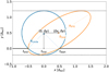 |
Fig. 2 Determining the simplest sheared disc model. The coordinate system is centred at (0, 0). The midpoint of the disc is shifted up to (0, δy). A circle (blue) is drawn with radius Rcircle (Eq. (3)). The midpoint of the disc is shifted to (δx, δy), shearing the circle into an ellipse (orange, Eqs. (4)–(6)). From this ellipse the disc parameters can be determined. |
4.1 Simple sheared disc model
To explore this grid in an intuitive manner, we define a Cartesian coordinate system, in eclipse duration space, centred on the midpoint of the eclipse (tmid = 0), with the x-axis aligned with the transit path of the star, and the y-axis with the impact parameter. We note that since we are proposing that the transverse velocity is positive and move in the x direction, larger x point to earlier times in the light curve. We thus want to find the simplest sheared disc that is bound by the transit duration, ∆ecl and is centred at (δx, δy).
The most obvious solution is simply a circle with Rdisc = 0.5 ∆ecl centred at (δx, δy) = (0, 0). Changing the impact parameter impacts the y-coordinate of the midpoint of the disc, which changes the size of the circular disc to a radius defined by Eq. (3) and as seen in Fig. 2. This is expressed as

If we also move the centre of the disc in the x-direction, we need to ensure that the resulting ellipse is still bound by tstart and tend at y = 0. To do this we shear the circle into an ellipse, with the transformation defined in Eq. (4) and (5), where s is the shear parameter defined in Eq. (6):


This shear transformation allows for the determination of the simplest possible ellipse produced from the sheared circle centred at (δx, δy), with a width of ∆ecl and passing through tstart and tend at a height of y = 0. The ellipse parameters must be determined for this grid point, which can in turn be mapped to the disc parameters. To determine the semi-major, aproj, and semi-minor, bproj, axes of the projected disc, we must determine the location of a vertex and co-vertex of the ellipse described. This can be done by noting that the vertex of an ellipse must fulfill the condition dR/dθ = 0, where θ is the parametric angle of the ellipse. To perform this operation, we initially defined the simple radius circle for the ellipse (see blue circle in Fig. 2) in parametric form in Eqs. (7) and (8), as follows:


We then apply the shearing as defined by Eqs. (4) and (5), as


The equation of the ellipse can be written as

Substituting Eqs. (9) and (10) into Eq. (11), then taking the derivative and setting it to 0 (dR/dθ = 0) provides the analytic definition (Eq. (12)) of a vertex of this ellipse:

This can, in turn be used with Eqs. (7) and (8) to determine the (x, y) coordinate of either aproj or bproj. The next vertex (either aproj if the angle defined by Eq. (12) defines bproj or vice versa) is at 9 + π/2. With the (x, y) coordinates of the vertices of the ellipse, we can determine aproj and bproj simply, using Eq. (13):

The tilt is obtained by choosing the vertex related to the aproj and using Eq. (14), expressed as

Finally, the inclination is determined by Eq. (15) as

With this process, it is possible to determine the simplest sheared disc that has its midpoint at (δx, δy) and passes through the points (±0.5,0). We are able to determine the size and orientation of the simplest disc that could cause an eclipse lasting ∆ecl given the centre of the disc. We note that in units of time, we need not concern ourselves with υt as this is simply a proportionality factor used to convert from sizes in terms of time to sizes in distance.
4.2 Extension of discs
There are two further points to consider after the disc determination in the previous section. The first is that five points are required to uniquely determine a given ellipse, so there are an infinite number of ellipses that are centred at (δx, δy) and intersect with (±0.5,0). The second is that while the circles defined by Rcircle are the smallest possible ‘circles’ that intersect with the eclipse boundaries, after shearing, the resulting ellipses are not necessarily the ellipse with the smallest semi-major axis; thus, the equations above do not provide the smallest possible discs. To extend the parameter space defined by the simplest sheared disc model and create a three-dimensional (3D) grid – with the position of the disc centre (δx, δy) and the radius scale of the disc, fR – we must be able to model this complete family of ellipses.We do so by introducing two scale factors, fx and fy. These scale factors are applied after shifting the midpoint from the origin to (0, δy). The circle is scaled into an ellipse, by scaling x and y in Eqs. (4) and (5), as described in Eq. (16) and visualised in Fig. 3:

Scaling in one direction, say y using fy, causes the newly formed ellipse to no longer pass through the points (±0.5,0). For this reason, a dependent scaling must be applied in the perpendicular direction, here x with fx, such that the newly formed ellipse once again passes through the points (±0.5, 0). fx can thus be defined by Eq. (17) as a function of fy, as follows:

Thus, fy is taken as an independent parameter, with fx compensating the effects of fy and being a dependent parameter for the ellipse.
We note that the introduction of these scaling factors modifies Eq. (12) into the general case described by Eq. (18):

Now it becomes possible to analytically determine every ellipse that has a midpoint at (δx, δy) and passes through the points (± 0.5, 0), by adding the scale factor, fy. Thus, we have established a 3D grid with parameters δx, δy, and fy.
4.3 Converting to a radius fraction
The grid defined above is constructed rapidly as it is determined analytically. However, fy is not an intuitive third dimension, as it has no obvious physical meaning. Thus, we need to convert fy into a the radius scale factor, fR = Rdisc/Rmin, which relates the size of the disc to its minimum radius, at each (δx, δy). This dimension drops from any radius scale factor, say ƒR,max down to fR,mm = 1 back up to ƒR,max. This is due to the fact that one can increase the size of the final disc either by stretching the simple circle horizontally, ƒx > ƒx | Rmin, or vertically, ƒy > ƒy |Rmm , as shown in Fig. 4. The analytical formulation of the Rdisc as a function of either ƒx or ƒy to determine Rmin, becomes too involved and, thus, it must be determined numerically. Initially a high-resolution grid is generated from the starting ƒx = ƒy = 1 (simplest sheared disc solution) that is extended in one direction with ƒx > 1 (ƒy < 1; wider ellipses) and with ƒy > 1 (ƒx < 1; taller ellipses) in the other direction. The ƒR grid is determined through linear interpolation of this ƒx – ƒy grid.
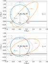 |
Fig. 3 Determining the scaled disc model. Top: ƒy > 1. Bottom: ƒy < 1. The coordinate system is centred at (0, 0). The midpoint of the disc is shifted up to (0, δy). A (blue) circle is drawn with radius Rcircle (Eq. (3)). The circle is then scaled in the y direction by ƒy and this scaling is compensated with a scaling in the x direction with ƒx (grey). The midpoint of the disc is then shifted to (δx, δy), shearing the ellipse to the proper midpoint (orange). From this ellipse, the disc parameters can be determined. |
4.4 Gradient analysis
Another source of information is the light-curve gradients measured as:  It should be noted that the light curve of a transiting ring system is not time-symmetric for most geometries (see Fig. 7, where the most obvious asymmetry is in the time central occultation approximately between −0.1 and 0.1 days). As described in Kenworthy & Mamajek (2015), the light-curve gradient is dependent on the size of the star, the local tangent of the ring edge and the direction of motion. This is characterised by Eq. (19), where the projected gradient, g(t), is defined by Eq. (21), T0 is the transmission at the ingress of the ring edge, and T1 is the transmission at the egress of the ring edge. We note that this equation is only valid when the ring edge boundary can be approximated as a straight line. It is expressed as
 (19)
(19)
For a given orientation, determined by δx, δy, i, and ϕ, an upper bound to the absolute gradient can be calculated by determining what the absolute gradient would be for a transition from fully transparent (T0 = 1) to fully opaque (T1 = 0). Given this upper bound on the gradient, it is possible to rule out a given disc geometry based on the light-curve gradients measured. Those measured gradients must be lower than the upper bounds for the geometry to represent a physically possible solution.
We determine the local tangents of the ring edges along the transit path of the star. To do so, we solve Eq. (16), in Cartesian coordinates, for  thereby producing Eq. (20):
 (20)
(20)
This local tangent can be converted to a projected gradient, g(x), by means of Eq. (21). This ensures that the projected gradient runs from 1 (perpendicular) to 0 (parallel):
 (21)
(21)
A visual representation of the time evolution of the local tangents and their respective projected gradients can be seen in Fig. 5. The pattern to note is that the projected gradient starts from the 1/s asymptote (see Eq. (20)) rising slowly before peaking at some value where the local tangent is perpendicular to the direction of motion (g(x) = 1). There is a steep drop to the time when the local tangent is parallel to the direction of motion (g(x) = 0), before the projected gradient rises to the same asymptotic value of 1/s.
The local tangents of the discs generated by the Shallot Explorer are determined for (x, 0). Also, x is a position in the eclipse duration, which is coupled to the measured light-curve gradient,  measured in L* day−1, time measured in days. The conversion is described in Eq. (22):
 (22)
(22)
Finally we note that the light-curve gradients are measured from as many data points that show this trend in the light curve as possible to increase the signal-to-noise ratio (S/N) of the measurement. This is done by fitting a straight line to the light curve data wherever an extended increase/decrease of flux is observed.
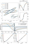 |
Fig. 4 Effects of ƒR on disc geometry. Top left: changes in disc shape and geometry. Top-upper right: evolution of inclination with ƒR. Top-lower right: evolution of tilt with ƒR. Middle: evolution of the theoretical maximum gradient with ƒR. Bottom left: evolution of ƒR with ƒx. Bottom right: evolution of ƒR with ƒx. We note that this disc is centred on (δx, δy) = (0.67, 0.47) in ∆ecl. |
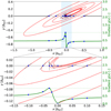 |
Fig. 5 Determining local tangents and projected gradients. Upper: full projected gradient curve outside and during the transit. Lower: part of the transit where the projected gradient changes significantly and rapidly. Note: the projected gradient is stable for relatively large |x| because the change in the local ring edge tangent is negligible with position (the left and right asymptote are 1/s as dictated by Eq. (20)). For small |x|, the projected gradient rises to some peak value (where the local tangent is perpendicular to motion), before quickly dropping to 0 (where the local tangent is parallel to motion), and then rising once more. In the lower panel, it appears that the local tangent rotates counterclockwise with time, which supports the sinusoidal definition of the projected gradient (Eq. (21)). |
4.5 Limiting the parameter space
The disc models and gradient analysis discussed in the previous sections describe an infinitely large parameter space described by (δx, δy, fR). To limit the parameter space we introduce two astrophysical restrictions.
4.5.1 Hill radius
An important stability criterion for the disc is that the disc remains stable under the gravitational interactions with the host star. To ensure an extended lifetime of the disc, Rdisc < 0.3 RHill, where RHill is the Hill radius defined by Eq. (23) (Quillen & Trilling 1998); then, a is the orbital semi-major axis, e is the eccentricity of the orbit, m is the mass of the companion, and M is the mass of the host star. This measurement is expressed as
 (23)
(23)
It is necessary to obtain information (a, m, M) that is not readily determined from the normalised light curve. This also means that the Hill radius restriction applies to the whole grid.
4.5.2 Gradients
Another consideration is that projected gradients determined from the measured light-curve gradients, must be less than the projected gradient upper limits derived from Eqs. (19)–(21). This is because the upper limit is based on a boundary from fully opaque (T = 1 ) to fully transparent (T = 0), and ring crossings will never produce steeper light-curve gradients and thus projected gradients. As the upper bound of a projected gradient is determined by its location on the x axis for a given geometry (see Fig. 5), the projected gradients measured from the light curve serve as a way to cut out all the unphysical geometries.
4.5.3 Visualisation
Figure 6 shows the evolution of valid grid points as the restrictions are applied to the grid; in particular, the disc radius is shown. In this case, a Hill radius limit of 2 ∆ecl is applied and a projected gradient is applied at a time, t = 0.45 ∆ecl, with a value g(t) = 0.1. We note that it is from this characteristic visualisation of the disc radii the Shallot Explorer derives its name from.
4.6 Computational considerations
To increase the computational efficiency of calculating the grid, several degeneracies and symmetries are exploited. For a given point (δx, δy), there exists a point (δx, −δy), (−δx, −δy) and (−δx, δy), that produce ellipses with the same disc radius and inclination, but with a different tilt. In disc radius and inclination the first quadrant can be reflected off the x and y axis to produce the four quadrants. Tilt requires an additional transformation after reflecting off the x/y axis. For quadrants 2 and 4 ϕ → 180 − ϕ, while quadrants 1 and 3 remain the same. This ensures the tilt is restricted from 0° to 180°, which is possible because an ellipse has an axis of symmetry that is aligned with the tilt. Finally, projected gradients can be reflected off the x-axis, but not the y-axis, thus requiring the first and second quadrant. This means that Rdisc, i, and ϕ are calculated for one quadrant, and gradients analysis is performed on two, effectively reducing the computation time to a significant extent.
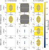 |
Fig. 6 Shallot visualisation of the disc radius. The first row shows the full extent of the grid with no restrictions applied. The second row shows the grid after applying just a Hill radius cut at 2 ∆ecl. The third row shows the grid after applying just a cut due to a projected gradient at t = 0.45 ∆ecl with a value of g(t) = 0.1. The fourth row shows the grid after applying both the projected gradient and Hill radius cut. Left: grid slice with ƒR = 2 when the disc is stretched horizontally. Middle: grid slice with the minimum radius disc (ƒR = 1). Right: grid slice with ƒR = 2 when the disc is stretched vertically. |
5 Light curve simulations
The transit of ring systems can be modelled to validate whether the geometry of a given grid point of the Shallot Explorer fits the data. These light curves are simulated using the pyPplusS package developed by Rein & Ofir (2019). It makes use of a Polygon plus Segments (P+S) algorithm to rapidly and accurately determine the area of a star that is blocked by a ringed planet. The package fixes the shape of the star to a circle with a radius of 1, which implies that the distances defined are in units of R*. It is possible to change the intensity profile of the star by applying one of the limb-darkening laws, which can be described with up to four parameters. The occulter is composed of two objects: the anchor body which is an opaque circle (T = 0) with any given size (0 is also possible); and a ring which has an inner radius, outer radius, transmission, tilt, and inclination. It is then possible to model the orbital motion of the occulter by passing in the (x, y) coordinate in the physical space in units of R*, centred on the midpoint of the star. The result is that for every given (x, y) position, pyPplusS is able to determine the relative intensity of the star (1 – when the occulter does not occult the star and 0 – when the star is fully blocked by an opaque object).
Light curves measure the relative flux of a star with respect to time, so the physical space must be converted to temporal space. This is done by firstly assuming that the path of the occulter across the face of the star (the transit chord) is a straight line, which means we can rotate the coordinate system such that the occulter’s y position is fixed, denoted as the impact parameter (for transits, we describe how this is justified in Appendix A). The x coordinate now tracks the motion across the transit chord, but this should be converted to time space by introducing a transverse velocity, υt, which is assumed to be constant during the transit of the occulting body and the maximum occultation time, δt, which is a time-shift parameter to align the light curve. We are then able to model light curves: (1) for planets by setting the transmission of the ring to T = 1; (2) discs by setting the planet and inner ring radius to zero; and (3) a ringed planet.
To extend the model to produce simulations of ring system transits, we ran the package multiple times. We initially ran it for a planet with no rings and then subsequently for each individual ring (with no planet). We then combined the light curves of each component. We note that this approach fails for small rings that are partially occulted by the anchor body itself and for transit geometries where the anchor body transits the star and there is a gap between the anchor body and the first ring. As we are primarily focused on very large ring systems, this effect is deemed negligible, especially considering that it is now possible to model ring system transits. We note that if we were to use enough rings, it would even be possible to model a quasi-continuous transmission profile of the disc-ring system. Figure 7 shows an example of a simulation produced in this way, with parameters listed in Table 2.
6 Comparisons to real data
To validate the effective parameter space reduction, the Shallot Explorer is used to determine a viable parameter space for candidate ring systems in the literature. In both cases, we used a relatively coarse Shallot Explorer grid that extends from δx = −1 → 1, δy = −1 → 1 and ƒR = 5 (h) → 1 → 5 (υ), where (h) is horizontal stretch and (υ) is vertical stretch. The bounds of δx, δy, and ƒR are chosen such that the extremities of the grid at ƒR = 1 can be cut away by the Hill radius restriction. This ensures that the exploration is complete.The grid has a final shape of (201, 201, 401), which is a resolution of (0.01, 0.01, 0.02). Two examples are explored in this work.
6.1 J1407b
J1407 b is a widely studied system that highlights the complexity of pinning down and characterising single eclipse systems that exhibit a complex sub-structure (see Fig. 8).
Kenworthy & Mamajek (2015) studied the light curve to fit a ring system and found a 36-ring solution with a reasonable fit (see Table 3). Subsequently mass and period limits were studied by Kenworthy et al. (2015), followed by constraints on the size and dynamics by Rieder & Kenworthy (2016). Due to nature of the eclipse, photographic plates were studied by Mentel et al. (2018), and a search for other potential transiting companions was performed by Barmentloo et al. (2021). ALMA data was taken to observe the ring system by Kenworthy et al. (2020), which led to the surprising conclusion that J1407 b is an unbound object that happened to transit J1407 at the right time. For the purposes of validating the Shallot Explorer, we set aside the conclusions reported by Kenworthy et al. (2020) and direct our attention to the models produced by Kenworthy & Mamajek (2015).
To carry out the gradient analysis, we set the eclipse duration to ∆ecl = 50.5 days, determined from the tend – tstart = 50.9 days of the modelled eclipse (green line from Fig. 8) and subtracting the diameter of the star (d* = 0.4 days). The transverse velocity is set to υt = 33 km s−1 and the limb darkening of the star to u = 0.8. To perform the right unit conversions, we set the star radius to R* = 0.9 R⊙. The measured light-curve gradients (time (t), light-curve gradient (d/(t)/dt), errors, and transmission change (T0 – T1)) are listed in Table 4.
Kenworthy & Mamajek (2015) and Mentel et al. (2018) showed that the ring system exhibited by J1407 b fills the Hill sphere; thus, we took RHill = 0.6 AU and converted it to the time space, yielding RHill = 0.621 ∆ecl. We also performed the gradient analysis twice: once excluding the measured transmission changes (i.e. setting (T0 – T1) = 1, which is more inclusive) and a second time including the measured transmission changes. To illustrate this, we rewrite Eq. (19) in terms of g(t) and introduce the transmission factor, fT = (T0 – T1). In the rest of this paper, ‘transmission scaling’ refers to the act of using the actual measured transmission factor, fT, instead of substituting unity (fT = 1), as follows:
 (24)
(24)
Now it is clear that ignoring the measured transmission ( fT = 1) provides the lowest possible g(t), which means the fewest ring system configurations are excluded. We also note that if, for any reason (e.g. sparse photometry), it is not possible to measure fT, then the value defaults to 1. This provides an inclusive analysis and by applying the measured ƒT, the analysis becomes more exclusive.
Once the gradient analysis and Hill sphere restriction have been performed, we use the χ2 goodness-of-fit (as described in Eq. (25)) to to rank the physically possible configurations. Here, o is the observed (measured) value, e is the expected value, and σ is the error on the measurement. It is expressed as
 (25)
(25)
The χ2 value is determined for each grid point (note: all points where the measured value is greater than the expected value are ignored as they are physically impossible). These points are then extracted and sorted by the χ2 value. We chose to investigate all solutions, finding that from the 16 200 801 explored grid points, only 1850 are physically possible. These solutions were then sorted by disc radius. Solutions with δy < 0 are ignored as they are degenerate (see Sect. 4.6). To visualise the distribution of these physical solutions, we introduce the normalised r.m.s.,  described in Eq. (26), where
  and
and  are the smallest and largest χ2 values measured respectively. This is expressed as
 (26)
(26)
The solutions are subsequently placed into five bins with a width of 0.2, running from  = 0.0−1.0 and the distribution of disc parameters is presented in Fig. 9. This figure demonstrates the complexity of the possible physical systems that could fit the light curve data.
The reason we performed the gradient analysis while ignoring the transmission factor is due to the large uncertainties involved in determining them. This is primarily due to the photometric data being too sparse to confidently measure a transmission change. To accurately determine fT for a particular light-curve gradient, we must have a flat-bottom before and after the gradient time (which, in most cases, is not available). This leads to the estimation of fT. We must take the largest upper bound of fT because underestimating it can lead to unphysical projected gradients (g(t) > 1).
The ring systems of both analyses are visible in Fig. 10 with projected gradient information shown in Fig. 11. Notice how there are some solutions which have a smaller disc radius than the original paper. This highlights the purpose of Shallot Explorer in finding physically smaller ring solutions.
Table 7 compares the smallest disc solution found by Shallot Explorer with a  < 0.2 to the solution determined by Kenworthy & Mamajek (2015).
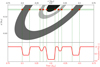 |
Fig. 7 Geometry of a transiting ring system with parameters described in Table 2. Top: ring system in grey scale, with the stellar transit path in green, with a red stellar disc. The vertical green dotted lines indicate when the stellar disc is moving behind a ring edge. Bottom: theoretical light curve for the ring system. Note: the projected gradient of the light curve is related to the geometrical tangent of the ring edge with the star and that the light curve drops or rises before the ring crossing because of the finite size of the star. |
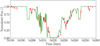 |
Fig. 8 J1407 light curve. The SuperWASP photometry of the star with the model of the ring system superimposed. The model parameters can be found in Table 3. This is a slightly modified version of the top panel of Fig. 4 from Kenworthy & Mamajek (2015). |
Ring model parameters for J1407 b from Kenworthy & Mamajek (2015).
407 measured light-curve gradients.
6.2 PDS 110
PDS 110 (HD 290380) is a young (~11 Myr old) T-Tauri star in the Orion OB1 Association. It exhibited two extended, deep eclipses with a duration of approximately 25 days, which were separated by about 808 days. These eclipses were studied by Osborn et al. (2017) and were interpreted as the result of the transit of a circumsecondary disc around an unseen companion, PDS 110 b. An observing campaign was subsequently setup to detect an expected transit event, but no such event occurred (Osborn et al. 2019). We focus on the ring models produced by Osborn et al. (2017).
The analysis follows the same steps as we undertook for J1407 (detailed in the previous section), but we limit the number of solutions investigated to 10 000. This is because as the number of solutions increases, they become so general that they end up meaningless. The Hill radius for PDS 110 is 0.69 AU and to do the gradient analysis the eclipse duration is set to ∆ecl = 25 days, the transverse velocity is set to υt = 27 km s−1, and the limb darkening of the star to u = 0.8. To perform the right unit conversions, we set the star radius to R* = 2.23 R⊙. The measured light-curve gradients (time (t), light-curve gradient (dI(t)/dt), errors, and transmission change (T0 – T1)) are listed in Table 6.
The ring systems of both passes are visible in Fig. 13 with projected gradient information shown in Fig. 14. We notice how all the solutions have a significantly smaller disc radius than the original model used. This demonstrates the use case of the Shallot Explorer.
As with J1407, we also show the distribution of the parameters for bins of  in Fig. 15. In Table 7, we see how the smallest disc with an
  , compares with the model determined by Osborn et al. (2017).
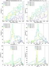 |
Fig. 9 J1407 disc property distributions. Each panel shows the distribution of a particular disc property, grouped by |


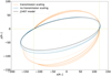 |
Fig. 10 J1407 disc models. The results of the Shallot Explorer are shown along with the original model for the J1407 disc (black). Solutions that ignore transmission scaling, |

7 Discussion and conclusions
The Shallot Explorer module of the BeyonCE package is an effective tool for exploring and visualising the parameter space spanned by circumsecondary discs. It produces a grid that is described with the offset of the centre of the disc with respect to the centre of the eclipse in time space, with a final dimension describing the size of the disc relative to the minimum possible size at that specific centre offset. The parameter space is still very large, but can be limited by two fundamental properties. The first is the Hill radius, which imposes a maximum size of the disc based on stability criteria for the object orbiting the host star. The second is the relationship between the light-curve gradients measured and the physical local tangent of the edge of the disc crossing the star. Implementing these two cuts effectively, significantly reduces the parameter space to much more manageable starting points for further analysis. Importantly, the Shallot Explorer makes no use of prior distributions. Instead, it is designed to explore the unbiased parameter space of everything that is physically possible. We are producing a systematic approach and defining the boundary between possible and not possible disc geometries based on the gradients as opposed to only minimising the radius of the disc.
Two examples were explored in this work. The first is J1407 b, an object with a very large ring system proposed. Using the information obtained from the light curve (light-curve gradients, eclipse duration, etc.) and from the orbits of the system (mass of the star, orbital mechanics), Shallot Explorer was capable of returning solutions of a similar geometry as those found by Kenworthy & Mamajek (2015) (see Table 7). The same analysis was done for the PDS 110 system, producing solutions that are significantly smaller than the proposed disc (see Table 7 and Fig. 13). This analysis generally provides a robust exploration of the disc orientations and in these particular cases (J1407b and PDS 110) reduces the parameter space to ~10% of our initial grid. Figure 9 and 15 show the distribution of each disc property for the valid configurations with a positive impact parameter, for J1407 and PDS 110, respectively. By ‘valid configurations’ we are referring to the solutions left over after applying the Hill radius and projected gradient cuts. We chose the positive impact parameter because we obtain the same disc solution by flipping the sign of the impact parameter and reflecting the tilt off the ϕ = 90° axis (as described in Sects. 2 and 4.6).
Both of these results suggest a different aspect of Shallot Explorer. The fact that J1407 b has such similar solutions implies that Shallot Explorer is able to find a solution that is determined by other means and that the solution found for the J1407 system is one of the smallest solutions given the light curve data. The fact that PDS 110 shows smaller solutions implies that Shallot Explorer is able to find solutions with a better fit than a focussed case study. The more Shallot Explorer is used on similar complex systems, the more evidence will support its application as the starting point in modelling complex light curves.
While the grid produced is linearly scalable, the implications do have hidden consequences. For instance, we can consider the light curve for J1407 b (Fig. 8): it shows no definitive eclipse duration as we are missing a clear ingress and egress and we also have no confirmation that the light curve remains steady outside of this time period. While not knowing the eclipse duration has no effect on the validity of the grid points, it does have an influence on the gradient cuts applied. This becomes obvious when looking at Eq. (22). The time measured changes with respect to the eclipse duration, which changes the maximum theoretical value that gradient could have. For gradients measured close to the ingress and egress, this will have a small effect. For gradients measured closer to the times when the local tangent of the ring edge is parallel and perpendicular to the direction of motion (between −0.1 and 0.1 in Fig. 5), the uncertainty in eclipse duration could have a very significant effect.
Another limitation that is not considered here is that every ring crossing produces four gradients: two sets of an ingress and an egress. This is not considered when making cuts to the parameter space, ensuring that the parameter space is larger than it would otherwise be. Shallot Explorer is thus inclusive of the correct solutions; however, determining the best-fit solutions (as described by Eq. (25)) is only a starting point when moving on to a light-curve fitting for a ring system.
It is also useful to investigate the Rdisc value at which the Shallot Explorer fails to produce viable results due to the breakdown of the first assumption:

BeyonCE will be supplemented with a second module that will be used for the fitting of the actual ring system transmissions itself, based on results exported from the Shallot Explorer or unique manual input from the user.
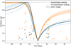 |
Fig. 11 J1407 projected gradients. The projected gradients are plotted for the ring system models depicted in Fig. 10. Note that the orange data points make use of ƒT and that the J1407 model (black) does not (ƒT = 1). |
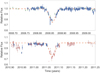 |
Fig. 12 Solutions that ignore transmission scaling, ƒT,x = 1, are in blue, and the solutions that do not are in orange. PDS 110 light curve. Top: first eclipse from 2008. Bottom: second eclipse from 2011. The red circles are data from KELT, the blue squares is data from SuperWASP, the green triangles are data from ASAS. The best fit eclipse model is over-plotted in orange with parameters in Table 5. This figure is extracted from the bottom left panels of Fig. 1 from Osborn et al. (2017). |
Ring model parameters for PDS110 from Osborn et al. (2017).
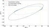 |
Fig. 13 PDS 110 disc models. The results of the Shallot Explorer are shown along with the original model for the PDS 110 disc (black). In blue, solutions that ignore transmission scaling, (T0 – T1)x = 1. In orange, the solutions that integrate it. Solutions that ignore transmission scaling, ƒT,x = 1, are in blue, and the solutions that do not are in orange. |
PDS 110 measured light-curve gradients.
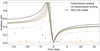 |
Fig. 14 PDS 110 projected gradients. The projected gradients are plotted for the ring system models depicted in Fig. 10. Note: the orange data points make use of fT and the PDS 110 model (black) does not (fT = 1). Solutions that ignore transmission scaling, fT,x = 1, are in blue, and the solutions that do not are in orange. |
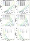 |
Fig. 15 PDS 110 disc property distributions. Each panel shows the distribution of that particular disc property that has been grouped by |


Literature versus Shallot Explorer model comparisons.
Acknowledgements
To achieve the scientific results presented in this article we made use of the Python programming language (Python Software Foundation, https://www.python.org/), especially the SciPy (Virtanen et al. 2020), NumPy (Oliphant 2006) and Matplotlib (Hunter 2007).
Appendix A Validity of exoring software geometry
The exoring code approximates the path of the star behind the rings with a straight line that is parallel to the x-coordinate of the ring coordinate system (line SC; see Figure A.1). In reality, for non-zero impact parameters, the path of the star behind the ring system follows an ellipse (assuming a circular orbit for the eclipser around the star), whose projected semimajor axis on the sky is the radius of the orbit of the eclipser about the star, a.
We estimate how close the approximation of the straight line path is to the correct orbital path by taking the most extreme case scenario: that of a disc that is face-on to the observer with an impact parameter y. In Figure A.1, S represents the star, P the centre of the disc, and RD is the radius of the disc seen face on to the observer. The straight line path lies along the line S C, where C is the point where the star leaves the disc. The orbital curved path is along SB, and the perpendicular distance from the x-axis to the star’s location is AB = y cos ϕ where ϕ is the orbital phase angle of P in its orbit around S.
Our goal is to calculate the distance BC, the distance between the idealised path and the orbital path. From geometry, ϕ can be calculated from triangle SPA as tan ϕ = x/a, which we approximate to ϕ = x/a and substitute into BC to get BC = yx2/(2a2). We substitute x2 = ( ) to obtain

We note that BC is zero both at y = 0 and y = RD, with a maximum value at  . We now have

The radius of the disc and the semimajor axis, a, are related through the radius of the Hill sphere:

Here, e is the eccentricity of P about S (taken to be zero), and m and M* are the masses of P and S, respectively.
The disc fills a fraction, ξ, of the Hill sphere RH so we have RD = ξRH and substituting into BCMAX we get

If we take the mass ratio of the star and planet to be 0.1, this equation is now

This shows that for the most extreme case, the difference in the paths is 2%, and for ring stability, typically ξ ≈ 1/3, resulting in a difference of much less than one percent for all realistic geometries.
We may consider the validity of the approximation of a constant velocity of the star behind the rings. The maximum velocity, υmax, of the star is when the star crosses the centre line of the disk SP at ϕ = 0, and the projected velocity on the sky plane, υ = υmax cos ϕ ~ υmax(1 – ϕ2/2). The fractional decrease in the velocity Δυ/υmax = ϕ2/2, and in the most extreme case crossing the full diameter of the disk this is where  , leading to

The fractional decrease in velocity is therefore

For ξ = 1/3 and m/M* = 0.1, this is approximately 0.6%, so we find that the assumption of constant velocity is reasonable.
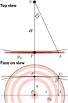 |
Fig. A.1 Sketch of geometry used in the exoring software. There are two views of the same system, indicating the relevant distances and quantities used in the derivation of the distance BC. |
References
- Alencar, S. H. P., Teixeira, P. S., Guimarães, M. M., et al. 2010, A&A, 519, A88 [NASA ADS] [CrossRef] [EDP Sciences] [Google Scholar]
- Ansdell, M., Gaidos, E., Hedges, C., et al. 2019, MNRAS, 492, 572 [Google Scholar]
- Barmentloo, S., Dik, C., Kenworthy, M. A., et al. 2021, A&A, 652, A117 [NASA ADS] [CrossRef] [EDP Sciences] [Google Scholar]
- Benisty, M., Bae, J., Facchini, S., et al. 2021, ApJ, 916, L2 [NASA ADS] [CrossRef] [Google Scholar]
- Borucki, W. J., Koch, D., Basri, G., et al. 2010, Science, 327, 977 [Google Scholar]
- Budaj, J. 2013, A&A, 557, A72 [NASA ADS] [CrossRef] [EDP Sciences] [Google Scholar]
- Cody, A. M., & Hillenbrand, L. A. 2018, AJ, 156, 71 [Google Scholar]
- Cody, A. M., Stauffer, J., Baglin, A., et al. 2014, AJ, 147, 82 [Google Scholar]
- Fischer, D. A., Howard, A. W., Laughlin, G. P., et al. 2014, Exoplanet Detection Techniques (Tucson: University of Arizona Press), 715 [Google Scholar]
- Handler, G. 2013, Planets, Stars and Stellar Systems (Berlin: Springer), 207 [CrossRef] [Google Scholar]
- Heinze, A. N., Tonry, J. L., Denneau, L., et al. 2018, AJ, 156, 241 [Google Scholar]
- Helled, R., Bodenheimer, P., Podolak, M., et al. 2014, in Protostars and Planets VI, eds. H. Beuther, R. S. Klessen, C. P. Dullemond, & T. Henning (Tucson: University of Arizona Press), 643 [Google Scholar]
- Howell, S. B., Sobeck, C., Haas, M., et al. 2014, PASP, 126, 398 [Google Scholar]
- Hunter, J. D. 2007, Comput. Sci. Eng., 9, 90 [NASA ADS] [CrossRef] [Google Scholar]
- Joy, A. H. 1945, ApJ, 102, 168 [Google Scholar]
- Kennedy, G. M., Kenworthy, M. A., Pepper, J., et al. 2017, R. Soc. Open Sci., 4, 160652 [NASA ADS] [CrossRef] [Google Scholar]
- Kenworthy, M. A., & Mamajek, E. E. 2015, ApJ, 800, 126 [NASA ADS] [CrossRef] [Google Scholar]
- Kenworthy, M. A., Lacour, S., Kraus, A., et al. 2015, MNRAS, 446, 411 [NASA ADS] [CrossRef] [Google Scholar]
- Kenworthy, M. A., Klaassen, P. D., Min, M., et al. 2020, A&A, 633, A115 [NASA ADS] [CrossRef] [EDP Sciences] [Google Scholar]
- Kochanek, C. S., Shappee, B. J., Stanek, K. Z., et al. 2017, PASP, 129, 104502 [Google Scholar]
- Kratter, K., & Lodato, G. 2016, ARA&A, 54, 271 [NASA ADS] [CrossRef] [Google Scholar]
- Lieshout, R. V., & Rappaport, S. A. 2018, Handbook of Exoplanets (Berlin: Springer), 1527 [CrossRef] [Google Scholar]
- Mamajek, E. E., Quillen, A. C., Pecaut, M. J., et al. 2012, AJ, 143, 72 [Google Scholar]
- Mentel, R. T., Kenworthy, M. A., Cameron, D. A., et al. 2018, A&A, 619, A157 [NASA ADS] [CrossRef] [EDP Sciences] [Google Scholar]
- Olah, K., Kővári, Z., Bartus, J., et al. 1997, A&A, 321, 811 [NASA ADS] [Google Scholar]
- Oliphant, T. 2006, NumPy: A guide to NumPy (USA: Trelgol Publishing) [Google Scholar]
- Osborn, H. P., Rodriguez, J. E., Kenworthy, M. A., et al. 2017, MNRAS, 471, 740 [Google Scholar]
- Osborn, H. P., Kenworthy, M., Rodriguez, J. E., et al. 2019, MNRAS, 485, 1614 [Google Scholar]
- Pollacco, D. L., Skillen, I., Collier Cameron, A., et al. 2006, PASP, 118, 1407 [NASA ADS] [CrossRef] [Google Scholar]
- Quillen, A. C., & Trilling, D. E. 1998, ApJ, 508, 707 [Google Scholar]
- Rappaport, S. 2012, ApJ, 752, 13 [NASA ADS] [CrossRef] [Google Scholar]
- Rappaport, S., Zhou, G., Vanderburg, A., et al. 2019, MNRAS, 485, 2681 [NASA ADS] [CrossRef] [Google Scholar]
- Rein, E., & Ofir, A. 2019, MNRAS, 490, 1111 [NASA ADS] [CrossRef] [Google Scholar]
- Ricker, G. R., Winn, J. N., Vanderspek, R., et al. 2015, J. Astron. Telesc. Instrum. Syst., 1, 014003 [Google Scholar]
- Ridden-Harper, A. R., Keller, C. U., Min, M., van Lieshout, R., & Snellen, I. A. G. 2018, A&A, 618, A97 [NASA ADS] [CrossRef] [EDP Sciences] [Google Scholar]
- Rieder, S., & Kenworthy, M. A. 2016, A&A, 596, A9 [NASA ADS] [CrossRef] [EDP Sciences] [Google Scholar]
- Rodono, M., Cutispoto, G., Pazzani, V., et al. 1986, A&A, 165, 135 [NASA ADS] [Google Scholar]
- Shappee, B. J., Prieto, J. L., Grupe, D., et al. 2014, ApJ, 788, 48 [Google Scholar]
- Teachey, A., Kipping, D. M., & Schmitt, A. R. 2018, AJ, 155, 36 [Google Scholar]
- Tonry, J. L., Denneau, L., Heinze, A. N., et al. 2018, PASP, 130, 064505 [Google Scholar]
- van Dam, D., Kenworthy, M., David, T., et al. 2019, AAS/Division Extreme Solar Systems Abstracts, 51, 322.10 [NASA ADS] [Google Scholar]
- van der Kamp, L., van Dam, D. M., Kenworthy, M. A., Mamajek, E. E., & Pojmanski, G. 2022, A&A, 658, A38 [NASA ADS] [CrossRef] [EDP Sciences] [Google Scholar]
- van Kooten, M. A. M., Kenworthy, M., & Doelman, N. 2020, MNRAS, 499, 2817 [NASA ADS] [CrossRef] [Google Scholar]
- van Werkhoven, T. I. M., Kenworthy, M. A., & Mamajek, E. E. 2014, MNRAS, 441, 2845 [NASA ADS] [CrossRef] [Google Scholar]
- Virtanen, P., Gommers, R., Oliphant, T. E., et al. 2020, Nat. Methods, 17, 261 [Google Scholar]
- Zanazzi, J. J., & Lai, D. 2017, MNRAS, 464, 3945 [NASA ADS] [CrossRef] [Google Scholar]
- Zieba, S., Zwintz, K., Kenworthy, M. A., & Kennedy, G. M. 2019, A&A, 625, L13 [NASA ADS] [CrossRef] [EDP Sciences] [Google Scholar]
All Tables
All Figures
|
Fig. 1 Disc parameters. Symbols are the same as in Table 1. Scale factors in the table are not included here as they are contained by Rdisc and i. |
| In the text | |
|
Fig. 2 Determining the simplest sheared disc model. The coordinate system is centred at (0, 0). The midpoint of the disc is shifted up to (0, δy). A circle (blue) is drawn with radius Rcircle (Eq. (3)). The midpoint of the disc is shifted to (δx, δy), shearing the circle into an ellipse (orange, Eqs. (4)–(6)). From this ellipse the disc parameters can be determined. |
| In the text | |
|
Fig. 3 Determining the scaled disc model. Top: ƒy > 1. Bottom: ƒy < 1. The coordinate system is centred at (0, 0). The midpoint of the disc is shifted up to (0, δy). A (blue) circle is drawn with radius Rcircle (Eq. (3)). The circle is then scaled in the y direction by ƒy and this scaling is compensated with a scaling in the x direction with ƒx (grey). The midpoint of the disc is then shifted to (δx, δy), shearing the ellipse to the proper midpoint (orange). From this ellipse, the disc parameters can be determined. |
| In the text | |
|
Fig. 4 Effects of ƒR on disc geometry. Top left: changes in disc shape and geometry. Top-upper right: evolution of inclination with ƒR. Top-lower right: evolution of tilt with ƒR. Middle: evolution of the theoretical maximum gradient with ƒR. Bottom left: evolution of ƒR with ƒx. Bottom right: evolution of ƒR with ƒx. We note that this disc is centred on (δx, δy) = (0.67, 0.47) in ∆ecl. |
| In the text | |
|
Fig. 5 Determining local tangents and projected gradients. Upper: full projected gradient curve outside and during the transit. Lower: part of the transit where the projected gradient changes significantly and rapidly. Note: the projected gradient is stable for relatively large |x| because the change in the local ring edge tangent is negligible with position (the left and right asymptote are 1/s as dictated by Eq. (20)). For small |x|, the projected gradient rises to some peak value (where the local tangent is perpendicular to motion), before quickly dropping to 0 (where the local tangent is parallel to motion), and then rising once more. In the lower panel, it appears that the local tangent rotates counterclockwise with time, which supports the sinusoidal definition of the projected gradient (Eq. (21)). |
| In the text | |
|
Fig. 6 Shallot visualisation of the disc radius. The first row shows the full extent of the grid with no restrictions applied. The second row shows the grid after applying just a Hill radius cut at 2 ∆ecl. The third row shows the grid after applying just a cut due to a projected gradient at t = 0.45 ∆ecl with a value of g(t) = 0.1. The fourth row shows the grid after applying both the projected gradient and Hill radius cut. Left: grid slice with ƒR = 2 when the disc is stretched horizontally. Middle: grid slice with the minimum radius disc (ƒR = 1). Right: grid slice with ƒR = 2 when the disc is stretched vertically. |
| In the text | |
|
Fig. 7 Geometry of a transiting ring system with parameters described in Table 2. Top: ring system in grey scale, with the stellar transit path in green, with a red stellar disc. The vertical green dotted lines indicate when the stellar disc is moving behind a ring edge. Bottom: theoretical light curve for the ring system. Note: the projected gradient of the light curve is related to the geometrical tangent of the ring edge with the star and that the light curve drops or rises before the ring crossing because of the finite size of the star. |
| In the text | |
|
Fig. 8 J1407 light curve. The SuperWASP photometry of the star with the model of the ring system superimposed. The model parameters can be found in Table 3. This is a slightly modified version of the top panel of Fig. 4 from Kenworthy & Mamajek (2015). |
| In the text | |
|
Fig. 9 J1407 disc property distributions. Each panel shows the distribution of a particular disc property, grouped by |
| In the text | |
|
Fig. 10 J1407 disc models. The results of the Shallot Explorer are shown along with the original model for the J1407 disc (black). Solutions that ignore transmission scaling, |
| In the text | |
|
Fig. 11 J1407 projected gradients. The projected gradients are plotted for the ring system models depicted in Fig. 10. Note that the orange data points make use of ƒT and that the J1407 model (black) does not (ƒT = 1). |
| In the text | |
|
Fig. 12 Solutions that ignore transmission scaling, ƒT,x = 1, are in blue, and the solutions that do not are in orange. PDS 110 light curve. Top: first eclipse from 2008. Bottom: second eclipse from 2011. The red circles are data from KELT, the blue squares is data from SuperWASP, the green triangles are data from ASAS. The best fit eclipse model is over-plotted in orange with parameters in Table 5. This figure is extracted from the bottom left panels of Fig. 1 from Osborn et al. (2017). |
| In the text | |
|
Fig. 13 PDS 110 disc models. The results of the Shallot Explorer are shown along with the original model for the PDS 110 disc (black). In blue, solutions that ignore transmission scaling, (T0 – T1)x = 1. In orange, the solutions that integrate it. Solutions that ignore transmission scaling, ƒT,x = 1, are in blue, and the solutions that do not are in orange. |
| In the text | |
|
Fig. 14 PDS 110 projected gradients. The projected gradients are plotted for the ring system models depicted in Fig. 10. Note: the orange data points make use of fT and the PDS 110 model (black) does not (fT = 1). Solutions that ignore transmission scaling, fT,x = 1, are in blue, and the solutions that do not are in orange. |
| In the text | |
|
Fig. 15 PDS 110 disc property distributions. Each panel shows the distribution of that particular disc property that has been grouped by |
| In the text | |
|
Fig. A.1 Sketch of geometry used in the exoring software. There are two views of the same system, indicating the relevant distances and quantities used in the derivation of the distance BC. |
| In the text | |
Current usage metrics show cumulative count of Article Views (full-text article views including HTML views, PDF and ePub downloads, according to the available data) and Abstracts Views on Vision4Press platform.
Data correspond to usage on the plateform after 2015. The current usage metrics is available 48-96 hours after online publication and is updated daily on week days.
Initial download of the metrics may take a while.