© The Authors 2024

1. Introduction

Theoretical considerations, reinforced in recent years by extensive numerical simulations, show that the dynamical evolution of a stellar system in its own gravitational field is characterized by three basic timescales.

The shortest of them, the dynamic time T_d ∼ (Gρ)^−1/2, where G is the gravitational constant and ρ is the mass-average density of the system, is associated with large-scale motions of matter in the early stages of system evolution. This parameter is also called the crossing time, as the return time of a body that has fallen from the surface of a homogeneous ball of density ρ into a hole passing along its diameter is equal to (3π/Gρ)^1/2.

According to Jeans (1915, 1919), the subsequent relaxation of the system to a quasi-stationary state in the smoothed, so-called regular gravitational field (see Hénon 1982; Binney & Tremaine 2008) is described by the collisionless Boltzmann equation for the distribution function f(r, v, t) in six-dimensional phase space,

$$\begin{array}{c}\hfill \frac{\partial f}{\partial t}+\mathit{v}\frac{\partial f}{\partial \mathit{r}}-\frac{\partial \mathrm{\Phi }}{\partial \mathit{r}}\frac{\partial f}{\partial \mathit{v}}=0,\end{array}$$(1)

supplemented by the Poisson equation for the conjoint potential Φ(r, t). The definition of a quasi-stationary state is often associated with the virial equation, which is valid for any set of N gravitating points in the center of mass coordinate system:

$$\begin{array}{c}\hfill \frac{1}{2}\frac{{\mathrm{d}}^{2}J(t)}{\mathrm{d}{t}^2}=2K(t)+W(t),\end{array}$$(2)

where

$$\begin{array}{c}\hfill \begin{array}{cc}J(t)={\sum }_1^N{m}_i{\mathit{r}}_i^2,\hfill & \\ \hfill & \\ K(t)={\sum }_1^N{m}_i{\mathit{v}}_i^2/2,\mathrm{and}\hfill & \\ \hfill & \\ W(t)=-G{\sum }_{i=1}^{N-1}{\sum }_{j=i+1}^N\frac{m_i{m}_j}{|{\mathit{r}}_i-{\mathit{r}}_j|},\hfill \end{array}\end{array}$$(3)

respectively, are the moment of inertia of the system and its kinetic and potential energies, whereas m_i, r_i(t), and v_i(t) are the mass, radius-vector, and the speed of the i-th star¹. The total mass of the star system M = ∑m_i and its total energy E are assumed to be given. If the motions occur in a limited region of space, then averaging Eq. (2) over time, we obtain the equality 2⟨K⟩+⟨W⟩ = 0, called the virial theorem (Landau & Lifshitz 1976). It seems reasonable to distinguish between the terms virial equation and virial theorem, since the former is strictly true at any stage of the evolution of a gravitating system, while the latter is only approximately valid under certain conditions.

Star clusters are not closed in space, but observations show that, over time, a state close to a quasi-stationary one is reached, for which the virial theorem is approximately satisfied. By marking the parameters of such a system with asterisks, we can accept

$$\begin{array}{c}\hfill 2K_{\ast }+W_{\ast }=0.\end{array}$$(4)

Within the framework of the approach discussed here, we should understand the quasi-stationary state as the virial equilibrium state (VES). The characteristic time interval for reaching VES is denoted as T_v. Some models for subsequent restructuring of the system have been described by Binney & Tremaine (2008, Chapt. 8) and further explored by Levin et al. (2008) and Benetti et al. (2014).

Finally, the third stage, the relaxation of the system’s core towards the Maxwell-Boltzmann state, takes even more time T_r. For half a century it was believed that this process is due solely to the irregular gravitational field of the system, which is defined as the difference between the real and smoothed fields (Ambartsumian 1938; Chandrasekhar 1942; Spitzer 1987). Since the spatial density of stars in galaxies is low, the main contribution to the process is made by pair collisions (close passages) of stars; it is taken into account by the non-zero collisional term on the right-hand side of Eq. (1). An explicit representation of this term for systems with Coulomb or gravitational interaction was given by Landau (1937). Research in recent decades has associated relaxation to a more efficient process of dynamic chaos (Gurzadyan & Savvidy 1984, 1986); the corresponding relaxation time T_r ≃ N^1/3T_d (according to Rastorguev & Sementsov 2006, the exponent is 1/5). Thermodynamic equilibrium is never reached already due to the long-range nature of the gravitational force (Lynden-Bell 1967; Levin et al. 2008, 2014; Benetti et al. 2014); in addition, the openness of the system manifests itself in its external parts.

With regard to the evolution at the second of the stages mentioned above, the nature of the observed fast ‘Maxwellization’ of star systems in a regular field remained unclear for a long time. The revival of research in this direction was initiated by Hénon (1964) and Lynden-Bell (1967); the latter proposed an appropriate stochastic mechanism, as he called it, violent relaxation. In the current understanding, this implies the importance of collective processes in systems with long-range interaction (Shu 1978; Levin et al. 2008, 2014; Gurzadyan & Kocharyan 2009; Giachetti & Casetti 2019). On the other hand, numerical simulations, starting with van Albada (1982) studies and up to Halle et al. (2019) and Sylos Labini & Capuzzo-Dolcetta (2020) recent calculations, gradually clarify the commensurate role of radial instabilities and initial density fluctuations that lead to the formation of local substructures of increasing size. Unlike T_d and T_r, no explicit representation of T_v in terms of the integral parameters of the system has been found so far, especially since it depends on the initial state. Quantification is hindered by the extreme complexity of combining the kinetic and Poisson equations.

In this connection, the virial equation merits more attention. It should be taken to a deeper level of description compared to the kinetic equation in one its form or another because the latter is inevitably formulated with finite accuracy, while the virial equation is due only to the fundamental fact that the potential energy in the gravitational interaction of a pair of point-like bodies is inversely proportional to the distance between them; in other words, it is a homogeneous function coordinates of degree −1. Among other things, the virial equation is valid for any, small or large, number of interacting points, while the accuracy of Eq. (1) drops as N decreases. For N ≫ 1, the collisionless Boltzmann equation is consistent with the virial equation in the sense that Eq. (2), in its continuous version, can be derived from Eq. (1).

Since the total energy of an isolated system E = K(t)+W(t) is conserved in time, Eq. (2) is usually written as

$$\begin{array}{c}\hfill \frac{1}{2}\frac{{\mathrm{d}}^{2}J(t)}{\mathrm{d}{t}^2}=2E-W(t).\end{array}$$(5)

For a gravitationally bound system, a necessary (but insufficient) stability condition is E < 0 (Chandrasekhar 1942, Sect. 5.1); here, we assume that this condition is satisfied. This picture of evolution is illustrated in Fig. 1 (see also Fig. 6.1 in Ciotti 2021). Equation (5) includes two unknown functions of time, and therefore, by itself, does not allow complete description of even the integral properties of the system. However, we can anticipate that it shall provide some information about the character of evolution and the corresponding time intervals. Lynden-Bell (1967) and Chandrasekhar & Elbert (1972) looked at this equation from a dynamical point of view under simple assumptions (see Sect. 3 below). The purpose of this investigation is to clarify the character of evolution under more general conditions.

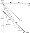Fig. 1. Representation of the dynamic evolution of a system on a diagram connecting kinetic, K, and potential energy, W. Evolution occurs along the straight line K(t)+W(t) = E, approaching on average a virial equilibrium state (VES). The thin lines correspond to fixed values of the virial ratio V given by Eq. (6). The letters C and H denote cold and hot configurations, which are characterized by the values K < |E| and K > |E|, respectively.

2. Signs of different behavior of two characteristic radii of the system

Usually, the degree of proximity to the state of virial equilibrium is given by the value of the virial ratio

$$\begin{array}{c}\hfill V(t)\equiv \frac{2K(t)}{|W(t)|}=2[1-\frac{E}{W(t)}],0\le V<2.\end{array}$$(6)

In view of Eq. (4), the values of the kinetic and potential energies in VES are:

$$\begin{array}{c}\hfill K_{\ast }=-E,W_{\ast }=2E,\end{array}$$(7)

so the equilibrium virial ratio V_* = 1. As the timescale in VES, we take T_* ≡ ℜ_*/v_* – the time of intersection of the mean harmonic radius ℜ_* of the system with the characteristic velocity v_*. The values of the last two follow from Eq. (7) and the definitions

$$\begin{array}{c}\hfill K_{\ast }\equiv \frac{1}{2}M{v}_{\ast }^2,W_{\ast }\equiv -\frac{G{M}^2}{2{\mathfrak{R}}_{\ast }}.\end{array}$$(8)

In this way we get:

$$\begin{array}{c}\hfill v_{\ast }={\left(\frac{2|E|}{M}\right)}^{1/2},{\mathfrak{R}}_{\ast }=\frac{G{M}^2}{4|E|},T_{\ast }=\frac{G}{4}{\left(\frac{M^5}{{2|E|}^3}\right)}^{1/2}.\end{array}$$(9)

The literature uses similar definitions with minor differences in numerical coefficients; the values adopted here are convenient for the following discussion. Notice that all these parameters are determined by the values of M and E. We can write the last part of Eq. (9) as T_* = (3/2πGρ_*)^1/2, where the characteristic density ${\rho }_{*}\equiv 3M/4\pi {\Re }_{*}^3$. As expected, the timescale T_* turns out to be on the order of dynamic time T_d. For a system supposedly in virial equilibrium, v_* and ℜ_* can be estimated directly from observations, and then the first two of formulas (9) allow us to find the total mass and energy of the system (Bahcall & Tremaine 1981; Binney & Tremaine 2008).

It is convenient to go in Eq. (5) to the requered quantities of a single physical nature, namely, the root mean square radius R(t) and the mean harmonic radius ℜ(t), which are defined as follows:

$$\begin{array}{c}\hfill \begin{array}{cc}{R}^2(t)\equiv \frac{1}{M}{\sum }_1^N{m}_i{\mathit{r}}_i^2,\hfill & \\ \hfill & \\ {\mathfrak{R}}^{-1}(t)\equiv \frac{2}{M^2}{\sum }_{i=1}^{N-1}{\sum }_{j=i+1}^N\frac{m_i{m}_j}{|{\mathit{r}}_i-{\mathit{r}}_j|},\hfill \end{array}\end{array}$$(10)

so that

$$\begin{array}{c}\hfill J(t)=M{R}^2(t),W(t)=-\frac{G{M}^2}{2\mathfrak{R}(t)},\end{array}$$(11)

and Eq. (5) takes the form:

$$\begin{array}{c}\hfill \frac{\mathrm{d}}{\mathrm{d}t}\left(R\frac{\mathrm{d}R}{\mathrm{d}t}\right)=\frac{\mathit{GM}}{2\mathfrak{R}(t)}-\frac{2|E|}{M}.\end{array}$$(12)

Finally, the parameters specified in Eq. (9) allow us to form dimensionless variables

$$\begin{array}{c}\hfill \tau \equiv t/T_{\ast },X\equiv \mathfrak{R}/{\mathfrak{R}}_{\ast },\mathrm{and}Y\equiv R/{\mathfrak{R}}_{\ast },\end{array}$$(13)

and bring the virial equation to a dimensionless form with all unit coefficients:

$$\begin{array}{c}\hfill \frac{\mathrm{d}}{\mathrm{d}\tau }\left(Y\frac{\mathrm{d}Y}{\mathrm{d}\tau }\right)=\frac{1}{X}-1,\end{array}$$(14)

while the definition (6) for the virial ratio becomes

$$\begin{array}{c}\hfill V(\tau )=2-X(\tau ),0<X(\tau )\le 2.\end{array}$$(15)

It is worth emphasizing an important fact that has not been discussed previously: Throughout the entire evolutionary process, the mean harmonic radius of a system with a negative total energy does not exceed twice the equilibrium value. The assertion follows from the definition ℜ/ℜ_* ≡ 2|E|/|W| and the inequalities K > 0, |E|< |W|. A clear evidence is that the lines V = constant in Fig. 1 do not intersect with the line corresponding to the given value E when the constant is greater than or equal to 2.

In view of the above, the approximation to virial equilibrium over time means that the harmonic radius of the system ℜ(t), changing in a relatively narrow range of values (0, 2ℜ_*), tends to its equilibrium value (Eq. (9)), that is X(τ)→1, the second derivative of R²(t) tends to zero, while the rms radius R(t) tends to a finite or, which is more likely, infinite value.

To demonstrate the theoretical possibility of the described scenario, and anticipating the discussion in the next section, we present in Fig. 2 the evolution of the harmonic and rms radii for a given behavior of the first radius, while the change in the second radius is calculated according to the virial Eq. (14). When solving this equation, we should take into account the interdependence of the initial values of X₀ and Y₀. Indeed, the initial system is a certain physical configuration with a specific value g₀ ≡ Y₀/X₀. As a given parameter, it is convenient to choose the initial value of the virial ratio V₀, and then X₀ = 2 − V₀ and Y₀ = g₀ ⋅ X₀. The choice of $Y_0^{\prime }$ is more complicated; we do not dwell on this, since only a representative example is considered. Specifically, it was assumed that X(τ) tends to 1, experiencing an exponential decay and oscillations with a period 2πT_* (see Eq. (23) below). It is noteworthy that Y²(τ) grows linearly as τ → ∞.

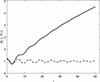Fig. 2. Change in the system rms radius Y(τ) over time (solid line) for a given behavior of the harmonic radius X(τ) (dashed line). The initial system is a homogeneous sphere with Y0/X0 = g0 given in Table 1; the initial virial ratio and speed are V0 = 0.75 and $Y_0^{\prime }=0$.

A. Rastorguev (priv. comm.) drew our attention to the fact that the practical constancy in time of the half-mass radius R_h in the Spitzer (1987) calculations of the evolution of stellar systems can be considered as a consequence of the above conclusion regarding the value of the harmonic radius. This is because the mean harmonic radius ℜ ≃ 2.5R_h within the framework of King’s models, which describe well the internal structure of the globular clusters.

Thus, the ratio of radii

$$\begin{array}{c}\hfill g(\tau )\equiv \frac{R(t)}{\mathfrak{R}(t)}=\frac{Y(\tau )}{X(\tau )}\end{array}$$(16)

can vary within wide limits, as opposed to the usual assumption of their equality or proportionality. In this regard, it is useful to estimate the parameter g for several continuous, for simplicity, density distributions that differ significantly from each other. Table 1 lists the corresponding data for systems with central symmetry. These distributions can be conditionally considered as instantaneous (but not sequential) states of a star cluster evolving in accordance with the kinetic and Poisson equations. To calculate the values given in the table, note that for a continuous distribution, the mass M(r) inside a sphere of radius r and the potential energy W are defined by the formulas

$$\begin{array}{c}\hfill \begin{array}{cc}\hfill M(r)& =4\pi {\int }_0^r\rho (r)r^2\mathrm{d}r,\hfill \\ \hfill & \\ \hfill W& =-4\pi G{\int }_0^{\infty }\rho (r)M(r)r\mathrm{d}r,\hfill \end{array}\end{array}$$(17)

so the analogs of Eqs. (10) are reduced, using Eq. (11), to

$$\begin{array}{c}\hfill \begin{array}{cc}\hfill R^2& =\frac{4\pi }{M}{\int }_0^{\infty }\rho (r)r^4\mathrm{d}r,\hfill \\ \hfill & \\ \hfill {\mathfrak{R}}^{-1}& =\frac{8\pi }{M^2}{\int }_0^{\infty }\rho (r)M(r)r\mathrm{d}r.\hfill \end{array}\end{array}$$(18)

As Table 1 shows, for the first three, relatively homogeneous distributions, the values of g are close to 1. Apparently, these density distributions are adequate only at the initial stage of evolution. The values of g remain of the same order for fairly significant deviations from the spherical symmetry of the density distribution, for example, towards ellipsoidality. A more important point is the density distribution in the outer region of the system. Still early theoretical research by von Hoerner (1957) indicate the formation of a power-law density distribution ρ(r)∝r^−α with exponent α ∼ 4 in the halo. This is supported by the thorough numerical modeling by Hénon (1964) and van Albada (1982), reinforced by the physical arguments of Trenti et al. (2005), along with further simulations of cluster evolution by Yangurazova & Bisnovatyi-Kogan (1984), Levin et al. (2008, 2014), Joyce et al. (2010), Sylos Labini (2013), Halle et al. (2019), and Sylos Labini & Capuzzo-Dolcetta (2020). The last two examples of Table 1 are just that. Example 4 is the system of Schuster (1883) and Plummer (1911), which was repeatedly used in connection with studies of globular star clusters. With density distributions as flat as in examples 4 and 5, the integrals for R diverge, so the g-factor is infinitely large.

The above models assume a more or less gradual change in density with distance from the center. An idea of the reverse behavior is given by a two-layer model with radii R₁, R₂ and densities ρ₁, ρ₂ in the central and outer zones, respectively. We do not present the corresponding formulas because of their cumbersomeness. The general conclusion is that at moderate values of the ratio ρ₁/ρ₂, the g-factor is still close to 1, and it is only when ρ₁/ρ₂ ≫ 1 and R₁/R₂ < 0.1 that a g value of more than 10 can be achieved.

Thus, it seems likely that relatively homogeneous systems at the initial stage of evolution are characterized by g(τ) on the order of 1, while the g-factor increases significantly during evolution as the dense core and extended halo of the system are formed.

3. Solutions for a given ratio of radii

In addition to the formal reason for the studying in Eq. (12) the dimensionless ratio of two unknown radii R(t) and ℜ(t), the function g(τ) plays an important role by setting the systematic behavior of the rms radius averaged over fast oscillations with a period on the order of dynamic time T_d (see the appendix for details).

In order to verify the oscillatory nature of the solutions of the virial equation, we write down Eq. (14) as

$$\begin{array}{c}\hfill \frac{\mathrm{d}}{\mathrm{d}\tau }\left(Y\frac{\mathrm{d}Y}{\mathrm{d}\tau }\right)=\frac{g(\tau )}{Y}-1,\end{array}$$(19)

and assume first that the ratio of the radii does not change with time. Lynden-Bell (1967) additionally linearized the corresponding equation; Chandrasekhar & Elbert (1972) found a rather complicated analytical solution to a nonlinear equation. Written in parametric form, the exact solution of Eq. (19) at g(τ)≡g₀ describes a classical cycloid:

$$\begin{array}{c}\hfill \{\begin{array}{cc}Y=g_0-acos\theta -bsin\theta ,\hfill & \\ \tau =g_0\theta -asin\theta -b(1-cos\theta ),\hfill & 0\le \theta <\infty ,\hfill \end{array}\end{array}$$(20)

whereas the mean harmonic radius of the system

$$\begin{array}{c}\hfill X(\tau )=Y(\tau )/g_0=1-(a/g_0)cos\theta -(b/g_0)sin\theta \end{array}$$(21)

oscillates around the equilibrium value X_* = 1. The constants a and b are determined by the initial state:

$$\begin{array}{c}\hfill a=g_0-Y_0,b=-Y_0·Y_0\prime .\end{array}$$(22)

It is convenient to proceed from three initial values, namely, the pair $(Y_0,Y_0^{\prime })$ and the virial ratio V₀; then, according to Eqs. (15) and (16), we have X₀ = 2 − V₀ and g₀ = Y₀/X₀.

Equation (6) shows that values of the kinetic energy less or greater than |E| correspond to virial ratio values less or greater than 1 (see Fig. 1); how it is accepted, we call the respective states of the system either cold or hot. The mean harmonic radius ℜ of the former state exceeds the equilibrium value ℜ_*, while we have ℜ < ℜ_* for the latter state. For example, the virial ratio of an isothermal sphere, regardless of its radius, is 3/2, so it should be classified as a hot unstable system.

A particular solution for V₀ = 0.20 (cold system) is shown in Fig. 3. The period of oscillations of the cycloid in real time is equal to g₀P_*, where

$$\begin{array}{c}\hfill P_{\ast }=2\pi T_{\ast }=\frac{\pi G}{2}{\left(\frac{M^5}{{2|E|}^3}\right)}^{1/2}=\sqrt{6\pi /G{\rho }_{\ast }},\end{array}$$(23)

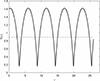Fig. 3. Changing the rms radius Y(τ) in a model with constant ratio Y/X ≡ g0 at initial values Y0 = 1.60, $Y_0^{\prime }$ = 0.10, V0 = 0.20. The dashed line corresponds to g0 = 8/9.

and ${\rho }_{*}=3M/4\pi {\Re }_{*}^3$ is the characteristic density of the cluster.

It is clear that the undamped, so-called homologous oscillations give only a preliminary description of the early evolution of a self-gravitating system. As noted at the end of the previous section, to estimate the characteristic time to reach virial equilibrium, it is necessary to take into account a progressive macroscopic inhomogeneity of the system. Accordingly, we must turn to a model with a time-varying ratio of radii R/ℜ. The appendix to this paper shows that the approximate solution of Eq. (19) with an arbitrary function g(τ), on which only the condition of its slow change on the timescale T_* is imposed, is a generalization of the classical cycloid, namely:

$$\begin{array}{c}\hfill \{\begin{array}{cc}Y=u(\theta )-a(\theta )cos\theta -b(\theta )sin\theta ,\hfill & \\ \tau =\theta u(\theta )-a(\theta )sin\theta -b(\theta )(1-cos\theta ),\hfill & 0\le \theta <\infty .\hfill \end{array}\end{array}$$(24)

Here, the base function u(θ) is given by the implicit equation u = g(θ ⋅ u) and the variable coefficients a(θ) and b(θ) depend on u(θ), that is, they are also given by the function g(τ). In the case of g(τ)≡g₀, we get u = g₀, the coefficients a, b become constant, and we return to the homologous model considered above. The physical meaning of representation in Eq. (24) is that the functions u(θ),a(θ) and b(θ) change relatively slowly, following g(τ), while their trigonometric factors precisely reflect these rapid variations of the rms radius around g(τ); the mean harmonic radius and virial ratio fluctuate around an equilibrium value 1. Our numerical examples show that in the immediate vicinity of the VES, the oscillation period slightly increases.

A more accurate approach, albeit not as informative as the analytical one, is the direct numerical solution of Eq. (19) for a given g(τ). Figure 4 gives an idea of a typical evolutionary pattern, in this case a hot system. The behavior of the mean harmonic radius X(τ) is not shown because, in view of Eq. (15), it is a reflection of V(τ) relative to the equilibrium level. We see several rapid initial fluctuations in both the rms radius and the virial ratio, however, later Y(τ) follows the given function g(τ), while V(τ) and X(τ) practically stabilize around the equilibrium level X_* = 1. This means that, over a period of two to three dozen of dynamic time intervals T_*, an almost equilibrium core with radius ℜ_* is formed in the system, while the surrounding halo, which determines the rms radius R(t), continues to expand.

Fig. 4. Solution of Eq. (19) with initial data V0 = 1.40, Y0 = 0.60, $Y_0^{\prime }$ = 0.10. Left: rms radius Y(τ) of the system (solid line) and g(τ) function (dashed line). Right: virial ratio V(τ) (solid line) and unit level corresponding to VES (dashed line).

The pattern of virial oscillations seen in the right Fig. 4 has the same character as that obtained by numerical simulation of the dynamics of a multiparticle system (see, e.g., Fig. 6 in Trenti et al. 2005). Fast oscillations are just a ringing against the backdrop of a slower reorganization of the system. Eventually, it is possible that after two dozen dynamic time periods T_* the harmonic radius of the system X(τ) will become close to 1; then, as the virial Eq. (14) shows, the further evolution of the root mean square radius of the system is described by simple law R(t)/ℜ_* = g(τ)≃(c₁τ + c₂)^1/2, where τ = t/T_* and c₁, c₂ are some dimensionless constants.

For control, it is also necessary to check the evolution of the system, which was initially in a virial equilibrium state. As can be seen in Fig. 5, the rapid oscillations of the radii and the virial ratio have disappeared, the rms radius Y(τ) still follows g(τ), while the quasi-equilibrium nucleus experiences only long-term weak oscillations. This result is expected.

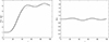Fig. 5. Solution of Eq. (19) with initial data V0 = 1.0, Y0 = 1.0, $Y_0^{\prime }$ = 0, corresponding to a virial equilibrium state. Details are the same as in Fig. 4.

The difference in the behavior of the system core and halo seems quite plausible, but we should not forget that in the context considered here it is partly determined by the specification of the g(τ) function. This prompted us to consider models with different types of g(τ); all cases, except for extremely hot systems, show the same behavior.

4. Concluding remarks

Since the time of H. Poincaré it has been known that motion in a system of several gravitating bodies is unstable; under certain initial conditions it becomes chaotic (Hénon & Heiles 1964). The virial equation contains only integral characteristics of a system of gravitating bodies, and the stability of its solutions remains to be studied. As for the dependence on the initial data, firstly on the virial ratio V₀, it manifests itself in a quite obvious way. Figures 4 and 5 show this when V₀ ≥ 1. On the other hand, we would generally expect that if V₀ is small, or even if V₀ = 0 when the system is completely cold and big in size, the initial oscillations in the virial ratio and both radii are relatively large, and the time to reach virial equilibrium increases. This behavior is confirmed both by extensive numerical simulations, in particular van Albada (1982), Trenti et al. (2005), and by our calculations. However, despite all the differences in the details, the general character of the evolution towards virial equilibrium of the system’s core remains unchanged.

The above consideration implies two features. First, the integral characteristics of the system fluctuate during two to three tens of dynamic time T_* until the virial ratio stabilizes near the equilibrium value V_* = 1. Secondly, the root mean square and mean harmonic radii vary differenly over time, so the common assumption that the radii are approximately equal or proportional is far from realistic. As already noted, the first conclusion agrees with the results of numerical simulation of self-gravitating systems at N ≫ 1. The second conclusion means a fundamentally different behavior of the moment of inertia of the system relative to the center of gravity and its potential energy.

Further details of the process of approaching the virial equilibrium state remain hidden when only the virial equation is analyzed. Additional data are desirable, at least in the form of approximate relationships between the integral characteristics of the system. On the other hand, the difference between evolutionary paths of the root mean square and the mean harmonic radii can be easily elucidated on the basis of both already performed and future numerical simulations.

Acknowledgments

The author is grateful to A.S. Rastorguev and the anonymous referee for useful comments. No new data were generated or analysed in support of this research.

References

Appendix A: Approximate analytical solution of the virial equation

A nonlinear differential equation of the second order

$$\begin{array}{c}\hfill Y[\frac{d}{d\tau }\left(Y\frac{\mathit{dY}}{d\tau }\right)+1]=g(\tau )\end{array}$$(A.1)

is considered in the domain τ ≥ 0 for a given non-negative function g(τ). The approach presented below, which goes back to the method of Van der Pol (1927), is widely used in the theory of oscillations.

We look for a solution in a parametric form:

$$\begin{array}{c}\hfill \{\begin{array}{cc}Y=u(\theta )-a(\theta )cos\theta -b(\theta )sin\theta ,\hfill & \\ \tau =\theta u(\theta )-a(\theta )sin\theta -b(\theta )(1-cos\theta ),\hfill & \theta \ge 0,\hfill \end{array}\end{array}$$(A.2)

where u(θ), a(θ) and b(θ) are some unknown functions slowly varying over an interval of length 2π. In particular, they can be constant. Specifically, we assume that |u′(θ)/u(θ)| ≪ 1, and similar inequalities hold for the coefficients a and b. Under this condition, the solution averaged over an interval of length 2π is

$$\begin{array}{c}\hfill ⟨Y(\theta )⟩=\frac{1}{2\pi }{\displaystyle {\int }_{\theta }^{\theta +2\pi }Y({\theta }^{\prime })d{\theta }^{\prime }\simeq u(\theta ),}\end{array}$$(A.3)

which determines the physical meaning of the function u(θ).

We have from Eqs. (A.2):

$$\begin{array}{c}\hfill \{\begin{array}{cc}dY/d\theta =u^{\prime }-a^{\prime }cos\theta +asin\theta -b^{\prime }sin\theta -bcos\theta ,\hfill & \\ d\tau /d\theta =u+\theta u^{\prime }-a^{\prime }sin\theta -acos\theta -b^{\prime }(1-cos\theta )-bsin\theta .\hfill \end{array}\end{array}$$(A.4)

According to the above condition, we can neglect here terms with derivatives, i.e. put

$$\begin{array}{c}\hfill \{\begin{array}{cc}{u}^{\prime }-a^{\prime }cos\theta -b^{\prime }sin\theta =0,\hfill & \\ \theta u^{\prime }-a^{\prime }sin\theta -b^{\prime }(1-cos\theta )=0,\hfill \end{array}\end{array}$$(A.5)

so that Eqs. (A.4) take the form:

$$\begin{array}{c}\hfill \{\begin{array}{cc}dY/d\theta =asin\theta -bcos\theta ,\hfill & \\ d\tau /d\theta =u-acos\theta -bsin\theta =Y.\hfill \end{array}\end{array}$$(A.6)

Dividing the top of Eqs. (A.6) by the bottom gives:

$$\begin{array}{c}\hfill Y\frac{\mathit{dY}}{d\tau }=asin\theta -bcos\theta .\end{array}$$(A.7)

Moreover, Eqs. (A.6) shows that the derivatives with respect to τ and with respect to θ are connected by the relation

$$\begin{array}{c}\hfill \frac{d}{d\tau }=\frac{1}{d\tau /d\theta }·\frac{d}{d\theta }=\frac{1}{Y}\frac{d}{d\theta }.\end{array}$$(A.8)

Applying this operator to Eq. (A.7), taking into account the first of Eqs. (A.2) and the condition of smallness of derivatives, we find:

$$\begin{array}{c}\hfill \begin{array}{cc}Y\frac{d}{d\tau }\left(Y\frac{\mathit{dY}}{d\tau }\right)=\frac{d}{d\theta }(asin\theta -bcos\theta )\simeq \hfill & \\ acos\theta +bsin\theta =u(\theta )-Y.\hfill \end{array}\end{array}$$(A.9)

Thus,

$$\begin{array}{c}\hfill Y[\frac{d}{d\tau }\left(Y\frac{\mathit{dY}}{d\tau }\right)+1]=u(\theta ),\end{array}$$(A.10)

which coincides with Eq. (A.1) provided that

$$\begin{array}{c}\hfill u(\theta )=g(\tau ).\end{array}$$(A.11)

Here it suffices to restrict ourselves to the first term in the representation of τ from Eqs. (A.2), so that the function u(θ) is found from the implicit equation

$$\begin{array}{c}\hfill u=g(\theta ·u).\end{array}$$(A.12)

Finally, given the known function u(θ), one can find coefficients a(θ) and b(θ) by solving the system of linear Eqs. (A.5) with respect to a′ and b′, and then integrating the results. Further technical details are quite obvious.

All Tables

All Figures

Fig. 1. Representation of the dynamic evolution of a system on a diagram connecting kinetic, K, and potential energy, W. Evolution occurs along the straight line K(t)+W(t) = E, approaching on average a virial equilibrium state (VES). The thin lines correspond to fixed values of the virial ratio V given by Eq. (6). The letters C and H denote cold and hot configurations, which are characterized by the values K < |E| and K > |E|, respectively.

In the text

	Fig. 2. Change in the system rms radius Y(τ) over time (solid line) for a given behavior of the harmonic radius X(τ) (dashed line). The initial system is a homogeneous sphere with Y0/X0 = g0 given in Table 1; the initial virial ratio and speed are V0 = 0.75 and $Y_0^{\prime }=0$.
In the text

	Fig. 3. Changing the rms radius Y(τ) in a model with constant ratio Y/X ≡ g0 at initial values Y0 = 1.60, $Y_0^{\prime }$ = 0.10, V0 = 0.20. The dashed line corresponds to g0 = 8/9.
In the text

	Fig. 4. Solution of Eq. (19) with initial data V0 = 1.40, Y0 = 0.60, $Y_0^{\prime }$ = 0.10. Left: rms radius Y(τ) of the system (solid line) and g(τ) function (dashed line). Right: virial ratio V(τ) (solid line) and unit level corresponding to VES (dashed line).
In the text

	Fig. 5. Solution of Eq. (19) with initial data V0 = 1.0, Y0 = 1.0, $Y_0^{\prime }$ = 0, corresponding to a virial equilibrium state. Details are the same as in Fig. 4.
In the text

References

- Ambartsumian, V. A. 1938, Ann. Leningrad St. Univ., 22, 19 [Google Scholar]
- Bahcall, J., & Tremaine, S. 1981, ApJ, 244, 805 [NASA ADS] [CrossRef] [Google Scholar]
- Benetti, F. P. C., Ribeiro-Teixeira, A. C., Pakter, R., & Levin, Y. 2014, Phys. Rev. Lett., 113, 100602 [NASA ADS] [CrossRef] [Google Scholar]
- Binney, J., & Tremaine, S. 2008, Galactic Dynamics (Princeton: Princeton Univ. Press) [Google Scholar]
- Chandrasekhar, S. 1942, Principles of Stellar Dynamics (Chicago: Univ. of Chicago Press) [Google Scholar]
- Chandrasekhar, S., & Elbert, D. D. 1972, MNRAS, 155, 435 [NASA ADS] [CrossRef] [Google Scholar]
- Ciotti, L. 2021, Introduction to Stellar Dynamics (Cambridge: Cambridge Univ. Press) [CrossRef] [Google Scholar]
- Giachetti, G., & Casetti, L. 2019, J. Stat. Mech., 1, 043201 [CrossRef] [Google Scholar]
- Gurzadyan, V. G., & Savvidy, G. K. 1984, Doklady AN SSSR, 277, 69 [NASA ADS] [Google Scholar]
- Gurzadyan, V. G., & Savvidy, G. K. 1986, A&A, 160, 203 [NASA ADS] [Google Scholar]
- Gurzadyan, V. G., & Kocharyan, A. A. 2009, A&A, 505, 625 [NASA ADS] [CrossRef] [EDP Sciences] [Google Scholar]
- Jeans, J. H. 1915, MNRAS, 76, 71 [Google Scholar]
- Jeans, J. H. 1919, Problems of Cosmogony and Stellar Dynamics (Cambridge: Cambridge Univ. Press) [Google Scholar]
- Joyce, M., Marcos, B., & Sylos Labini, F. 2010, AIP Conf. Proc., 1245, 955 [NASA ADS] [CrossRef] [Google Scholar]
- Halle, A., Colombi, S., & Peirani, S. 2019, A&A, 621, A8 [NASA ADS] [CrossRef] [EDP Sciences] [Google Scholar]
- Hénon, M. 1964, Ann. Astrophys., 27, 83 [Google Scholar]
- Hénon, M. 1982, A&A., 114, 211 [Google Scholar]
- Hénon, M., & Heiles, C. 1964, AJ, 69, 73 [NASA ADS] [CrossRef] [Google Scholar]
- Landau, L. D. 1937, J. Exper. Theor. Phys., 7, 203 [Google Scholar]
- Landau, L. D., & Lifshitz, E. M. 1976, Theoretical Physics. vol. I, Mechanics, 3rd ed. (Elsevier) [Google Scholar]
- Levin, Y., Pakter, R., & Rizzato, F. B. 2008, Phys. Rev. E, 78, 021130 [CrossRef] [Google Scholar]
- Levin, Y., Pakter, R., Rizzato, F. B., Teles, T. N., & Benetti, F. P. C. 2014, Phys. Rep., 535, 1 [CrossRef] [Google Scholar]
- Lynden-Bell, D. 1967, MNRAS, 136, 101 [Google Scholar]
- Plummer, H. C. 1911, MNRAS, 71, 460 [Google Scholar]
- Rastorguev, A. S., & Sementsov, V. N. 2006, Astron. Lett., 32, 14 [NASA ADS] [CrossRef] [Google Scholar]
- Schuster, A. 1883, Br. Assoc. Rep., 470, 427 [Google Scholar]
- Shu, F. H. 1978, ApJ, 225, 83 [NASA ADS] [CrossRef] [Google Scholar]
- Spitzer, L., Jr. 1987, Dynamical Evolution of Globular Clusters (Princeton: Princeton Univ. Press) [Google Scholar]
- Sylos Labini, F. 2013, MNRAS, 429, 679 [Google Scholar]
- Sylos Labini, F., & Capuzzo-Dolcetta, R. 2020, A&A, 643, A118 [EDP Sciences] [Google Scholar]
- Trenti, M., Bertin, G., & van Albada, T. S. 2005, A&A, 433, 57 [NASA ADS] [CrossRef] [EDP Sciences] [Google Scholar]
- van Albada, T. S. 1982, MNRAS, 201, 939 [NASA ADS] [CrossRef] [Google Scholar]
- Van der Pol, B. 1927, Lond. Edinb. Dublin Philos. Mag. J. Sci., 2, 978 [Google Scholar]
- von Hoerner, S. 1957, ApJ, 125, 451 [NASA ADS] [CrossRef] [Google Scholar]
- Yangurazova, L. R., & Bisnovatyi-Kogan, G. S. 1984, Astrophys. Space Sci., 100, 319 [CrossRef] [Google Scholar]