| Issue |
A&A
Volume 686, June 2024
|
|
|---|---|---|
| Article Number | A129 | |
| Number of page(s) | 14 | |
| Section | Interstellar and circumstellar matter | |
| DOI | https://doi.org/10.1051/0004-6361/202348761 | |
| Published online | 05 June 2024 | |
The dense and non-homogeneous circumstellar medium revealed in radio wavelengths around the Type Ib SN 2019oys★
1
Racah Institute of Physics, The Hebrew University of Jerusalem,
Jerusalem
91904,
Israel
e-mail: itai.sfaradi@mail.huji.ac.il
2
Department of Astronomy, The Oskar Klein Center, Stockholm University,
AlbaNova,
10691
Stockholm,
Sweden
3
Astrophysics, Department of Physics, University of Oxford,
Keble Road,
Oxford
OX1 3RH,
UK
4
Jodrell Bank Centre for Astrophysics, School of Physics and Astronomy, The University of Manchester,
Manchester
M13 9PL,
UK
5
Astrophysics Group, Cavendish Laboratory,
19 J. J. Thomson Ave.,
Cambridge
CB3 0HE,
UK
6
Center for Interdisciplinary Exploration and Research in Astrophysics (CIERA), Northwestern University,
1800 Sherman Ave.,
Evanston,
IL
60201,
USA
7
The Oskar Klein Centre, Department of Physics, Stockholm University, Albanova University Center,
106 91
Stockholm,
Sweden
8
Department of Particle Physics and Astrophysics, Weizmann Institute of Science,
234 Herzl St,
7610001
Rehovot,
Israel
Received:
28
November
2023
Accepted:
5
March
2024
Context. Mass loss from massive stars, especially towards the end of their lives, plays a key role in their evolution. Radio emission from core-collapse supernovae (SNe) serves as a probe of the interaction of the SN ejecta with the circumstellar medium (CSM) and can reveal the mass-loss history of the progenitor.
Aims. We aim to present broadband radio observations of the CSM-interacting SN 2019oys. SN 2019oys was first detected in the optical and was classified as a Type Ib SN. Then, ~100 days after discovery, it showed an optical rebrightening and a spectral transition to a spectrum dominated by strong narrow emission lines, which suggests strong interaction with a distant, dense, CSM shell.
Methods. We modelled the broadband, multi-epoch radio spectra, covering 2.2 to 36 GHz and spanning from 22 to 1425 days after optical discovery, as a synchrotron emitting source. Using this modelling, we characterised the shockwave and the mass-loss rate of the progenitor.
Results. Our broadband radio observations show strong synchrotron emission. This emission, as observed 201 and 221 days after optical discovery, exhibits signs of free–free absorption from the material in front of the shock travelling in the CSM. In addition, the steep power law of the optically thin regime points towards synchrotron cooling of the radiating electrons. Analysing these spectra in the context of the SN-CSM interaction model gives a shock velocity of 11 000 km s−1 (for a radius evolution of ~∆t0.8, where ∆t is the time since optical discovery) and an electron number density of 4.1 × 105 cm−3 at a distance of 2.6 × 1016 cm. This translates to a high mass-loss rate from the progenitor massive star of 10−3 M⊙ yr−1 for an assumed wind of 100 km s−1 (assuming a constant mass-loss rate in steady winds). The late-time radio spectra, 392 and 557 days after optical discovery, show broad spectral peaks. We show that this can be explained by introducing a non-homogeneous CSM structure.
Key words: circumstellar matter / stars: mass-loss / supernovae: general / supernovae: individual: SN 2019oys / radio continuum: general
The reduced data are available at the CDS via anonymous ftp to cdsarc.cds.unistra.fr (130.79.128.5) or via https://cdsarc.cds.unistra.fr/viz-bin/cat/J/A+A/686/A129
© The Authors 2024
 Open Access article, published by EDP Sciences, under the terms of the Creative Commons Attribution License (https://creativecommons.org/licenses/by/4.0), which permits unrestricted use, distribution, and reproduction in any medium, provided the original work is properly cited.
This article is published in open access under the Subscribe to Open model. Subscribe to A&A to support open access publication.
1 Introduction
Mass-loss from massive stars, that is, stars with MZAMS ≥ 8 M⊙ (zero-age main sequence mass of the star; MZAMS ), has a significant impact on their luminosity, lifetime, composition, and mass (e.g. Langer 2012). The mass lost from the massive star, either via winds or other mass-loss mechanisms (e.g. violent mass eruptions, binary interaction), forms a circumstellar medium (CSM) surrounding the massive star. Towards the end of its life, before the massive star explodes as a core-collapse supernova (CCSN), mass-loss can heavily influence the fate of the star and the resulting supernova (SN; e.g. Smith 2014). Despite its importance, mass loss at this last stage of stellar evolution is still highly unconstrained empirically.
Observations of CCSNe across the electromagnetic spectrum show a wide variety of properties. In the optical, distinct features in the SN spectral lines are used to classify CCSNe as sub-types (Filippenko 1997). Hydrogen-rich SNe, such as Type II SNe, are considered to be a result of the explosion of a massive star that retained its hydrogen envelope in its final stages. Stripped-envelope SNe (Types Ib and Ic), on the other hand, lack hydrogen spectral features and are the result of massive stars that lost their hydrogen envelopes (and in some cases even their helium envelope) in some sort of enhanced mass loss at the end of their lives (Gal-Yam 2017).
Radio observations of CCSNe probe the interaction between the SN ejecta and the CSM around the SN progenitor star (Chevalier 1982) and thus play a key role in revealing the mass-loss history of massive stars. While it is well established that the emission in radio from CCSNe is synchrotron emission that originates at the interaction region (Chevalier 1981; Chevalier & Fransson 2006; Weiler et al. 2002), there are variations between different CCSNe in the observed radio emission. For example, most SNe exhibit clear, self-absorbed synchrotron radio spectra (Chevalier 1998); however, some SNe (e.g. SN 1979C, Weiler et al. 1991; SN 1993J, Weiler et al. 2007) show steep power laws in the optically thick regime that point towards a spectrum associated with free–free absorption (FFA). This implies a more dense CSM around the massive progenitor star. Furthermore, steep power laws in the optically thin regime can arise from electron cooling either by synchrotron and/or inverse Compton cooling (e.g. SN 2012aw, Yadav et al. 2014; SN 2013df, Kamble et al. 2016; SN 2020oi, Horesh et al. 2020; SN 2016X, Ruiz-Carmona et al. 2022).
While it is common to assume a spherical, homogeneous CSM structure, deviations from this simple scenario have been observed in several CCSNe. Some SNe (e.g. SN 2014C; Anderson et al. 2017) exhibit a double peak in their radio light curve, suggesting that the SN ejecta interact with two separate CSM shells deposited in two separate mass-loss stages. Equipartition analysis of the radio spectral peaks of SN 2004C (DeMarchi et al. 2022) suggested a shock wave that initially interacts with an inner, relatively flat, density profile, and later with an outer ~r–2 profile. Panchromatic, optical, and radio observations of the Type Ib SN 2019tdf (Zenati et al. 2022) point towards a scenario of an SN ejecta interacting with a spherically asymmetric CSM, potentially disc-like. Some SNe exhibit broader radio spectral peaks. These broad peaks are associated with CSM inhomogeneities caused by variations in the distribution of relativistic electrons and/or the magnetic field strength within the synchrotron source. Radio observations of such broad peaks (e.g. SN 2003L, Soderberg et al. 2005; PTF11qcj, Björnsson & Keshavarzi 2017; Master OT J120451.50+265946.64, Chandra et al. 2019) shed light on variable mass-loss processes in the massive star’s final stages. Such variations from the typical synchrotron spectra and light curve can reveal deviation from the simple spherical CSM structure around the progenitor (which is the standard assumption) and can be caused, for example, by variable mass loss from the progenitor during its evolution.
Here, we present broadband radio observations of SN 2019oys. SN 2019oys (otherwise known as ZTF19abucwzt) was first detected on August 28, 2019 (JD = 2458723.98), with the Palomar Schmidt 48-inch (P48) Samuel Oschin Telescope as part of the Zwicky Transient Facility (ZTF) survey (Bellm et al. 2019; Graham et al. 2019; Sollerman et al. 2020). The SN was reported to the Transient Name Server (TNS1) on August 29, 2019, with the first detection of a host-subtracted magnitude of 19.14 ± 0.12 mag (in the g band). It is positioned in the spiral galaxy CGCG 146-027 NED01 and the J2000.0 coordinates of SN2019oys are α = 07h07m59s.26 and δ = +31°39′55″3. The distance to the source (based on its redshift, ɀ = 0.0165; Sollerman et al. 2020) is 73.2 ± 3.7 Mpc (where we adopted 5% uncertainty on this distance based on the distances published in the NED2 catalogue). SN 2019oys was discovered during the decline of the optical light curve and was first classified as a Type Ib SN. Then, about 100 days after optical discovery, it showed a re-brightening in the g and r bands. Deep Keck spectra (Sollerman et al. 2020) obtained at the re-brightening phase revealed a plethora of narrow, high-ionisation lines, including coronal lines. The evolution of the optical light curve and the makeover of the spectrum suggests an onset of strong CSM interaction at late times (~ 100 days after optical discovery).
The paper is structured as follows. In Sect. 2, we present our comprehensive radio observations of SN2019oys conducted with the Karl G. Jansky Very Large Array (VLA) and the Arcminute Microkelvin Imager - Large Array (AMI-LA). In Sect. 3, we model the first two radio spectra as arising from a blast-wave interaction with a spherical and homogeneous CSM structure. We also consider electron cooling effects and analsze the temporal evolution of the detailed 15.5 GHz light curve. In Sect. 4, we discuss the indications of a non-homogeneous CSM structure seen in the late-time radio spectra. Our conclusions are discussed in Sect. 5.
2 Radio observations
As part of our regular monitoring campaign for CCSNe, we first observed the field of SN 2019oys in radio wavelengths with the AMI-LA (Zwart et al. 2008; Hickish et al. 2018) on September 19, 2019, about 22 days after optical discovery. We detected a point source at the position of SN 2019oys with a flux level of 0.35 mJy at a central frequency of 15.5 GHz. Follow-up observations in the 15.5 GHz band were conducted using AMI-LA, and multi-wavelength observations were performed using the VLA.
2.1 The Arcminute Microkelvin Imager – Large Array
The AMI-LA is a radio interferometer comprised of eight 12.8 m diameter antennas producing 28 baselines that extend from 18 m up to 110 m in length and operate with a 5 GHz bandwidth; these are divided into eight channels around a central frequency of 15.5 GHz. This results in a synthesised beam of ~30 arcsec.
Observations of SN 2019oys were initially reduced, flagged, and calibrated using reduce_dc, a customised AMI-LA data-reduction software package (Perrott et al. 2013). Phase calibration was conducted using short interleaved observations of J0823+2223, while daily observations of 3C286 were used for absolute flux calibration. Additional flagging was performed using the common astronomy software applications (CASA; McMullin et al. 2007). Images of the field of SN 2019oys were produced using the CASA task CLEAN in an interactive mode. We fitted the source in the phase centre of the images with the CASA task IMFIT and calculated the image rms with the CASA task IMSTAT. We estimate the error of the peak flux density to be a quadratic sum of the error produced by CASA task IMFIT and 10% calibration error. The flux density at each time is reported in Table A.1.
2.2 The Karl G. Jansky Very Large Array
We observed the field of SN 2019oys with the VLA on several epochs starting on January 10, 2020. The observations (under our DDT programmes VLA/20A-421 and VLA/21A-394; PI Horesh) were performed in the S (3 GHz), C (5 GHz), X (10 GHz), Ku (15 GHz), K (22 GHz), and Ka (33 GHz) bands. The VLA was in C configuration during the first and second observations on March 16 and April 5, 2020, in the more extended B configuration in the third observation on September 23, 2020, and in the hybrid A → D configuration on March 7, 2021.
We calibrated the data using the automated VLA calibration pipeline available in the CASA package. Additional flagging was conducted manually when needed. Our primary flux density calibrator was 3C286, while J1215+1654 was used as a phase calibrator. Images of the SN 2019oys field were produced using the CASA task CLEAN in an interactive mode. Each image was produced using data from within the VLA bands, resulting in different spectral resolutions for the different bands. We also produced images of the full band data for each epoch.
Our observations showed a source at the phase centre (besides the S -band observations of the first two epochs), which we fitted with the CASA task IMFIT. The image rms was calculated using the CASA task IMSTAT. A summary of the flux density at different observing times and frequencies, for the full band images, are reported in Table A.1. We estimate the error of the peak flux density to be a quadratic sum of the error produced by the CASA task IMFIT, and a 10% calibration error.
2.3 The Very Large Array Sky Survey
In addition to the observations conducted by us as reported above, the field of view around the SN position was covered, with a central frequency of 3 GHz, by the VLA under the initiative of the Very Large Array Sky Survey (VLASS; Lacy et al. 2020) on April 22, 2019 (epoch 1.2), and December 3, 2021, (epoch 2.2). Examining the cutout images using the Canadian Initiative for Radio Astronomy Data Analysis (CIRADA3) reveals no point-source emission at the position of the SN on epoch 1.2; this was about four months prior to the optical discovery with 3σ rms of 0.39 mJy, and we thus set a limit on the possible contamination of the SN emission from a pre-existing radio source. On the other hand, the image obtained on epoch 2.2,823 days after optical discovery, shows a point source with a flux level of 3.4 ± 0.4 mJy (assuming 10% calibration error).
3 Modeling of the radio data: A spherical and homogeneous CSM structure
In the simple (spherical and homogeneous CSM structure) SN-CSM interaction model (Chevalier 1981, 1998), the radio emission observed from an SN is attributed to the interaction between the SN ejecta and the CSM. This plowing of the SN ejecta into the CSM generates a shock wave. In the shock front, electrons are accelerated to relativistic velocities, there is a power-law energy distribution (N = N0 E−p; where N is the density of relativistic electrons per unit energy, N0 is a constant, and p is the power-law index), and magnetic fields are enhanced. A fraction of the shockwave energy is deposited in relativistic electrons (єe), and a fraction of the shockwave energy is converted to magnetic fields (єB). The relativistic electrons are gyrating in the presence of the magnetic fields, and they radiate the synchrotron emission observed in radio wavelengths. Part of the emission can be absorbed by synchrotron self-absorption (SSA; Chevalier 1998) and/or FFA (Weiler et al. 2002). The synchrotron self-absorbed spectrum exhibits an optically thick regime of Fν ∝ V5/2, a radio spectral peak, and an optically thin regime of Fν ∝ v–(p–1)/2 (assuming no electron cooling). For electrons that are gyrating in a thin shell with a volume filling factor of f at a radius of R, in the presence of a constant magnetic field, B, the full spectral shape is described in Chevalier(1998).
A typical assumption is that the magnetic energy density, B2/8π, is a fraction, єB, of the post-shock energy,  . For a CSM that was deposited by constant mass loss from the progenitor via a steady wind with velocity υw, the density structure is ρ ~ Ṁ/ (υwr2), where Ṁ is the mass-loss rate. Assuming that the radius evolution with time is given by a power law, R ~ Δtm (where Δt is the time since optical discovery) results in a shock velocity of υsh = mR/Δt, which gives

External FFA can take place as discussed in many cases (e.g. Weiler et al. 2002; Chevalier & Fransson 2006; Horesh et al. 2012; Nayana et al. 2018) and was observed for several SNe (e.g. SN 1979C; Weiler et al. 1991, SN 1993J; Weiler et al. 2007, SN2013df; Kamble et al. 2016). This attenuates the optically thick regime of the synchrotron self-absorbed spectrum by a factor of  , where the optical depth for FFA (see e.g. Horesh et al. 2012) is

where Te is the temperature of the electrons in the CSM and EM is the integral of the electron density along the line of sight in units of cm–6pc. Assuming a spherical density profile (r–2) gives

where n*, is the density of the electrons at r*. Substituting into Eq. (2) gives4
![$\matrix{ {{\tau _{{\rm{ff}}}} = 0.76{m^3}{{\left( {{{\dot M\left[ {{{10}^{ - 6}}{M_ \odot }{\rm{y}}{{\rm{r}}^{ - 1}}} \right]} \over {{v_{\rm{w}}}\left[ {10{\rm{km}}{{\rm{s}}^{ - 1}}} \right]}}} \right)}^2}{{\left( {{{{T_{\rm{e}}}} \over {{{10}^5}{\rm{K}}}}} \right)}^{ - 1.35}}} \hfill \cr {{{\left( {{{{v_{{\rm{sh}}}}} \over {{{10}^4}{\rm{km}}{{\rm{s}}^{ - 1}}}}} \right)}^{ - 3}}{{\left( {{v \over {5{\rm{GHz}}}}} \right)}^{ - 2.1}}{{\left( {{{\Delta t} \over {10{\rm{Day}}}}} \right)}^{ - 3}}} \hfill \cr } $](/articles/aa/full_html/2024/06/aa48761-23/aa48761-23-eq6.png)
3.1 Our radio dataset
Early radio observations of SN 2019oys, taken with AMI-LA on Δt = 22 and 26 days, show a low emission level of ~0.3 – 0.4 mJy at 15.5 GHz (see right panel of Fig. 1). After a gap of about six months in observations, we triggered AMI-LA following the late-time CSM interaction observed in the optical. The flux measured from the SN at the same frequency had increased significantly to a level of ~10 mJy. The spectrum obtained with the VLA on Δt = 201 days revealed a broadband, optically thick emission up to the spectral peak at ~20 GHz. However, due to the lack of spectral coverage at high frequencies (≥36 GHz), we do not detect the optically thin emission to its full extent at that epoch. A full optically thick to thin spectrum is observed on Δt = 221 days. Two additional broadband VLA spectra obtained on Δt = 392 and 557 days are exhibiting extremely broad spectral peaks (see left panel of Fig. 1). Such broad peaks cannot be explained by a shockwave interaction with a spherical and homogenous CSM structure.
In Sect. 3.2, we analyse the early spectra (on Δt = 201 and 221 days) by assuming they arise from an SN ejecta interacting with a simple homogeneous CSM shell, as described above in the SN-CSM model. We then discuss the possibility of electron cooling (namely synchrotron cooling) and its effect on the physical parameters (i.e. R, B, and as a result, υsh and Ṁ) in Sect. 3.3. We examine the atypical, slow, temporal evolution of SN 2019oys through its detailed 15.5 GHz observations with AMI-LA (see Sect. 3.4). We discuss the analysis of the late-time spectra (on Δt = 392 and 557 days) showing broad spectral peaks in Sect. 4.
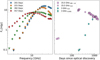 |
Fig. 1 Radio observations of SN 2019oys with VLA and AMI-LA (see Sect. 2). The left panel shows the broadband spectra obtained with the VLA in this work on four different epochs. The right panel shows the 15.5 GHz light curve obtained with AMI-LA (square markers) and the VLA (circle markers), and a 3 GHz light curve obtained by our VLA (circle markers) and VLASS (diamond marker) observations. The 3σ rms upper limits obtained by the VLA are marked with triangles. |
3.2 Single-epoch modelling of the synchrotron spectra
The functional form of a synchrotron self-absorbed spectrum can be described by its observed peak flux density, Fv,a, the synchrotron self-absorption frequency (at which the spectrum peaks), νa, and the power-law index of the optically thin regime, β (Chevalier 1998; Weiler et al. 2002):
![${F_v} = 1.582 \times {F_{v,{\rm{a}}}}{\left( {{v \over {{v_{\rm{a}}}}}} \right)^{{5 \over 2}}}\left( {1 - \exp \left[ { - {{\left( {{v \over {{v_{\rm{a}}}}}} \right)}^{ - \left( {{5 \over 2} + \beta } \right)}}} \right]} \right).$](/articles/aa/full_html/2024/06/aa48761-23/aa48761-23-eq7.png)
This two-power-law spectrum will be attenuated, in the case of external FFA, by a factor of
![$\exp \left[ { - {{\left( {{v \over {{v_{{\rm{ff}}}}}}} \right)}^{ - 2.1}}} \right,]$](/articles/aa/full_html/2024/06/aa48761-23/aa48761-23-eq8.png)
where νff is the FFA frequency that can be defined by Eq. (4).
We next model the first two radio spectra obtained by the VLA with the two-power-law model described above by fitting the spectra on Δt = 201 and 221 days to Eq. (5). Since we do not observe the optically thin part of the spectrum on Δt = 201 days to high enough frequencies, we cannot determine the power law of the optically thin regime. Thus, in all further analysis, we first fit the spectrum on Δt = 221 days and apply its fitted spectral slope to the fitting process of the spectrum on Δt = 201 days. For the spectrum on Δt = 221 days, the free parameters are the peak flux density, Fν,a, its frequency, νa, and the optically thin power-law index, β (we assume only SSA for now). We use emcee (Foreman-Mackey et al. 2013) to perform Markov chain Monte Carlo (MCMC) analysis to determine the posterior probability distributions of the parameters of the fitted model (and use flat priors). Based on the results of our fit (shown in the left panel of Fig. 2), we find that on Δt = 221 days Fv,a = 13.5 ± 0.6 mJy, νa = 19.7 ± 0.5 GHz, and β = 2.0 ± 0.2 (giving a reduced χ2 of 2.19 for 15 degrees of freedom; DOF; and a p value of 0.005). On Δt = 201 days, the peak flux density is 17.8 ± 0.5 mJy, and its frequency is 22.8 ± 0.3 GHz (giving a reduced χ2 of 1.59 for 16 DOF, and a p value of 0.06).
This model fails to describe the rise of the optically thick regime and to match the flux density upper limit at 3 GHz (see left panel of Fig. 2). Furthermore, setting a significance level of α = 0.05, the p value of the first epoch does not rule out that such a two-power-law model can describe the data. However, this is not the case for the second epoch, which resulted in a p value <0.05. Since this model fails to reproduce the optically thick regime, we try to accommodate it by assuming that there is an additional absorption mechanism, that is, external FFA by the material in front of the shock.
We fit these two spectra with Eq. (5) multiplied by  , where the free parameters are the same as the ones we used above plus the FFA frequency νff. We use emcee to perform an MCMC analysis and determine the posterior probability distributions of the parameters of the fitted model (and use flat priors). Based on the results of our fit (shown in the right panel of Fig. 2), we find that on Δt = 221 days Fν,a = 13.6 ± 0.7 mJy, νa = 17.9 ± 0.6 GHz, β = 1.7 ± 0.2, and νff = 3.5 ± 0.4 GHz (giving a reduced χ2 of 0.58 for 14 DOF, and a p value of 0.89). On Δt = 201 days the peak flux density is 17.4 ± 0.5 mJy, its frequency is 21 .5 ± 0.4 GHz, and the FFA frequency is 2.6 ± 0.5 GHz (giving a reduced χ2 of 0.69 for 15 DOF and a p value of 0.8).
Since the model of external FFA + SSA requires the additional free parameter we also applied the Bayesian information criterion (BIC) for model selection. This criterion considers the model with the highest likelihood but penalises models with more free parameters to avoid the issue of over-fitting. We find, for Δř = 201 days, that for the SSA-only model the BIC is 31.3; for the SSA + FFA model, the BIC is 19.2 (ΔBIC201 days = 12.1) for Δt = 221 days; for the SSA-only model, the BIC is 41.6; and for the SSA + FFA model, the BIC is 19.8 (∆BIC221 days = 21.8). The difference between the BIC of the two models is relatively large (∆BIC > 10 for both epochs); thus, the SSA+FFA model is strongly favoured (see e.g. the discussion in Raftery 1995) Furthermore, the SSA+FFA model describes the rise of the optically thick regime better than the model without the additional FFA term for both epochs. It also matches the flux density upper limit at 3 GHz, despite the fact that we did not force it in our fitting procedure. We thus note that external FFA in addition to the internal SSA is a more probable scenario than just SSA. However, it is important to note that while FFA is evident in the observed radio spectra, the peak flux density and frequency change only up to 2σ between the two models.
Assuming a spherical and homogeneous synchrotron self-absorbed source, the physical parameters of the shock, such as its radius and magnetic field strength, are given by the peak flux density and its frequency (Eqs. (11) and (12) in Chevalier 1998). We assume equipartition (ϵe = ϵB = 0.1; Scott & Readhead 1977; Chevalier 1998; Barniol Duran et al. 2013; however, see below) and an emission filling factor of f = 0.5. We also assume that cooling effects, such as inverse-Compton (IC) and/or synchrotron cooling, are not in effect (however, synchrotron cooling is in effect; see relevant analysis in Sect. 3.3). In that case, the power-law index of the energy distribution, p, is given by the spectral index of the optically thin power law β via β = (p − 1) /2. The fitted parameters under the SSA + FFA model translate to a radius of (3.5 ± 0.2) × 1016 cm, a magnetic field of 2.53 ± 0.09 G, and p = 4.4 ± 0.4 on ∆t = 221 days. On ∆t = 201 days, we infer R = (3.3 ± 0.2) × 1016 cm and B = 2.98 ± 0.07 G.
Assuming constant expansion (i.e. m = 1; we discuss the validity of this assumption and the expected physical properties under shock deceleration in Sect. 3.3) of the shock front, υsh = R/∆t, the shock velocity is (1.9 ± 0.1) × 104 km s−1 on both epochs. Using Eq. (1) and a assuming wind velocity of 100 km s−1, we find a mass-loss rate of Ṁ = (1.9 ± 0.3) × 10−4 and (1.6 ± 0.1) × 10−3 M⊙ yr−1 on ∆t = 201 and 221 days, respectively. The most likely progenitors of Type Ib SNe, He-stars are expected to experience mass loss at rates of 10−4−10−7 M⊙ yr−1 (Smith 2014). Thus, the mass-loss rates we infer from the radio spectral peaks are notably high. We note that deviations from equipartition (mostly ϵe > ϵe) have been observed in several CCSNe (e.g. SN 2011dh, Horesh et al. 2013; SN 2013df, Kamble et al. 2016; SN 2020oi, Horesh et al. 2020). ϵe/ϵB = 10 and 100 will reduce the inferred radius and shock velocity by 11% and 23%, respectively, and the magnetic field strength by 38% and 62%, respectively. The mass-loss rate will increase by a factor of 3.8 for ϵB = 0.01 and a factor of 14 for ϵB = 0.001 (assuming ϵe = 0.1).
A useful way to compare the radio properties of SNe is by examining the phase space of peak spectral luminosity and its frequency times the observed peak time for individual SNe. Lines of equal shock velocity and mass-loss rate are also plotted in this diagram (also called Chevalier’s diagram; Chevalier 1998). Figure 3 shows a Chevalier’s diagram with the position of SN 2019oys according to the radio spectral peak using the spectrum on ∆t = 201 and 221 days with other Type Ib and IIn SNe. In this diagram, we also plot lines of equal velocity and mass-loss rate assuming the same assumption made above and p = 3. This assumption should be taken with care in the case of SN 2019oys, as we observed optically thin spectral slopes that indicate p > 3. However, since most CCSNe show p ≃ 3, we find this assumption more suitable for comparison with other CCSNe. As seen from this plot, SN 2019oys is one the brightest SNe observed in radio wavelengths. SN 2019oys is also slower than all Type Ib SNe. However, the velocity comparison to other Type Ib SNe is not straightforward as it is measured at a late time, when usually the shock velocities from Type Ib SNe are measured at earlier times after the explosion. At late times, the shock accumulates mass, which can slow it down significantly. We further discuss the temporal evolution of SN 2019oys in Sect. 3.4.
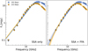 |
Fig. 2 Modelling of radio spectra obtained by VLA on ∆t = 201 and 221 days after optical discovery. The left panel shows the fitting of Eq. (5) to the spectra, assuming SSA as the only absorption mechanism. The right panel shows the fitting of Eq. (5) multiplied by Eq. (6) to the spectra, assuming that the absorption is due to both SSA and FFA by the material in front of the shock. Both fits also show shaded lines uniformly drawn from the posteriors of the fitted parameters. |
3.3 Electron cooling
Typically, the power-law index of the electron energy distribution, p, is much smaller (typically p = 2.5–3.5 for CCSNe; see e.g. Chevalier 1998) than the value of p = 4.4 ± 0.4 we infer for ∆t = 221 days. Such a high spectral slope can be an indication of cooling effects such as synchrotron and/or inverse-Compton (IC) cooling (see e.g. SN 2012aw, Yadav et al. 2014; SN 2013df, Kamble et al. 2016; SN 2020oi, Horesh et al. 2020). The synchrotron cooling frequency is

where me is the electron mass, c is the speed of light, qe is the charge of the electron, and σT is the Thomson cross-section. We find, based on Eq. (7) and the values of magnetic fields we give in Sect. 3.2, that vSyn_cool ≤ 2 GHz for both ∆t = 201 and 221 days, and therefore synchrotron cooling is important in our analysis. We do not test for IC cooling since its frequency is highly dependent on the bolometric luminosity of which we do not have any knowledge (see e.g. Chevalier & Fransson 2006; Horesh et al. 2020).
Taking synchrotron cooling into consideration, the spectral slope of the optically thin regime is now β = p/2; thus, we can derive p = 3.4 ± 0.4 for ∆t = 221 days (remember that due to lack of coverage at high frequencies, we use this value of p for both epochs). This translates, using the same analysis used in Sect. 3.2, to the following: R = (2.4 ± 0.1) × 1016 cm and B = 1.78 ± 0.04 G on ∆t = 201 days; and R = (2.6 ± 0.2) × 1016 cm and B = 1.51 ± 0.05 G on ∆t = 221 days. Assuming constant expansion of the shock front, υsh = R/∆t, the shock velocity is (1.4 ± 0.1) × 104 km s−1 in both ∆t = 201 and 221 days. From Eq. (1) (assuming υw = 100 km s−1), we derive a mass-loss rate of (6.7 ± 0.3) and (5.9 ± 0.4) × 10−4 M⊙ yr−1, for ∆t = 201 and 221 days, respectively. These are lower values of mass-loss rate (corresponding to lower density) than inferred without taking electron cooling into consideration (see Sect. 3.2). The inferred electron temperature in the wind is (7 ± 3) and (3 ± 1) × 104 K for ∆t = 201 and 221 days, respectively. A self-consistency check shows that, using the parameters inferred assuming synchrotron cooling, the cooling frequency is ≤ 1.3 GHz for both epochs, and therefore is important for the interpretation of the shock physical parameters.
When calculating the shock velocity, we assumed a constant expansion. However, our model suggests that during the first 200 days since the explosion the shock swept up ~0.05 M⊙, which can cause significant shock deceleration. The evolution of the radius between ∆t = 201 and 221 days, given the values inferred above and their uncertainties, are in agreement with values of m between 0.6 and 1. Taking m = 0.8 (similarly to what was seen in SN 1993J, Bartel et al. 2002, and what was taken from other works; e.g., Bietenholz et al. 2021) results in υsh = (1.1 ± 0.1) × 104 km s−1. We also derive corrected mass-loss rates of (1.0 ± 0.5) × 10−3 and (9.2 ± 0.6) × 10−4 M⊙ yr−1 for ∆t = 201 and 221 days, respectively. Finally, the corrected electron temperature in the wind is (4 ± 2) × 104 and (1 .8 ± 0.6) × 104 K for ∆t = 201 and 221 days, respectively.
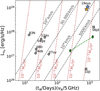 |
Fig. 3 Chevalier diagram of SN 2019oys (blue star marker for ∆t = 201 days and an orange star marker for ∆t = 221 days) with other Type Ib (grey circles) and IIn (grey squares) SNe. Also plotted for reference (green diamonds) are the two peaks observed in the 15.7 GHz light curve of SN 2014C (Anderson et al. 2017) which showed similar behaviour to SN 2019oys in the optical. The diagram shows the peak spectral radio luminosity, |

3.4 Temporal evolution
Most of the frequencies observed with the VLA for SN 2019oys do not have sufficient temporal coverage to analyse their temporal evolution. However, our Ku band observations with the VLA and AMI-LA (15.5 GHz) spread from a few weeks to almost two years after optical discovery (right panel of Fig. 1). In the following section, we analyse the light curve of SN 2019oys in the 15.5 GHz band.
We examined the temporal evolution of the SN by testing a two-power-law model such as the one introduced in Eq. (5):
![${F_v}(\Delta t) = 1.582{F_{v,a}}{\left( {{{\Delta t} \over {{t_a}}}} \right)^a}\left( {1 - \exp \left[ { - {{\left( {{{\Delta t} \over {{t_a}}}} \right)}^{ - (a + b)}}} \right]} \right),$](/articles/aa/full_html/2024/06/aa48761-23/aa48761-23-eq12.png)
where Fv,a is the peak flux at time ta, and a and b are the power laws of the rising and declining regimes of the light curve, respectively. We fit the two-power-law model shown in Eq. (8) to the 15.5 GHz observations. The free parameters are the peak flux Fv,a, its time ta, and the two power-law indices, a and b. We use emcee to perform an MCMC analysis to determine the posterior probability distributions of the parameters of the fitted model (and use flat priors). Based on the results of our fit (shown in Fig. 4), we find that Fv,a = 9.8 ± 0.4 mJy, ta = 187 ± 30 days,  and b = 0.71 ± 0.07. This results in χ2 = 15.9 for 26 DOF (p-value = 0.97). The observed decline rate of the 15.5 GHz light curve is atypical for CCSNe. In the simple SN-CSM model, assuming interaction with a spherical and homogeneous CSM shell, with a density structure of r−2, and free expansion, we expect a decline rate of t−1 (for p = 3, in our case of p = 3.4 ± 0.4 we expect t−1.2±0.2; Chevalier 1998). This discrepancy can be explained by an interaction with a more complex CSM structure at late times (see a detailed discussion on CSM inhomogeneities in Sect. 4).
While the decline of the light curve is well constrained, the peak flux density, its time, and the rising power law are based on the two early data points. Since the AMI-LA beam is large (~30 arcsec), it is possible that there is underlying emission from a diffusive background that contaminates our AMI-LA observations (and not the VLA observations thanks to its high resolution). Thus, while our late-time observations will not be affected too much by such contamination (as it is at most a few percent of the observed flux), it is possible that the two early observations are highly contaminated by a diffusive background. Therefore, we do not make use of these parameters to infer the physical properties of the shock and its surroundings.
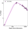 |
Fig. 4 Modelling of 15.5 GHz light curve obtained with VLA and AMI-LA. The light curve was fitted with a two-power-law model. Shaded lines are uniformly drawn parameters from the posterior probability distributions of the fitted parameters. |
4 Inhomogeneities in the CSM
Broad radio spectral peaks have been observed previously in several SNe (e.g. SN2003L, Soderberg et al. 2005; PTF 11qcj, Björnsson & Keshavarzi 2017; Master OT J120451.50+265946.6, Chandra et al. 2019). We also observe broad spectral peaks in SN 2019oys on ∆t = 392 and 557 days. Such broad peaks cannot be explained using the standard SN-CSM interaction model with a homogeneous r−2 CSM structure, and they are usually attributed to inhomogeneities in the CSM structure caused by variations in the distribution of relativistic electrons and/or the magnetic field strength within the synchrotron source (Björnsson 2013; Björnsson & Keshavarzi 2017). Since the shock accelerates the electrons in the CSM and also enhances the magnetic fields, a non-homogeneous CSM structure can result in a varying magnetic field across the emitting region. Thus, a way of introducing a non-homogeneous CSM structure to the synchrotron source is by applying a varying magnetic field.
Björnsson (2013) suggested that the magnetic field has a probability distribution of a power law, P(B) ~ B−α, between B0 and B1 (and zero elsewhere). Therefore, if the synchrotron spectrum for a given magnetic field B is Fv (R, B) (Eq. (1) in Chevalier 1998; assuming no cooling effects), then the total spectrum observed for a non-homogeneous CSM is given by

We next fit Eq. (9) to the spectra on days 392 and 557 after optical discovery, where the free parameters are the radius of the emitting shell, R, and the parameters of the magnetic field probability distribution, B0, B1, and α. In Sect. 3.2, we state that the electron power-law index is p = 3.4 ± 0.4. Since we do not observe the optically thin regime at sufficiently high frequencies in the last two epochs, we use this value of p in our analysis below.
We use emcee (Foreman-Mackey et al. 2013) to perform an MCMC analysis and determine the posterior probability distributions of the parameters of the fitted model (and use flat priors5). Based on the results of our fit for ∆t = 392 (shown in Fig. 5), we find that R = (3.4 ± 0.2) × 1016 cm, B0 = 0.82 ± 0.03 G, B1 ≳ 4 G, and α = 6.0 ± 0.5. Based on the results of our fit for ∆t = 557 (shown in Fig. 5), we find that R ≳ 5 × 1016 cm, B0 ≲ 0.45 G,  , and
, and  . Lines representing uniformly drawn parameters from the posteriors of the fitted parameters are plotted in Fig. 5. The shock velocity, assuming m = 0.8, is (0.8 ± 0.1) × 104 km s−1 at ∆t = 392 days and ≳0.8 × 10⁴ km s−1 on ∆t = 557 days. This points towards a deceleration of the shock when compared to the velocities we infer on ∆t = 201 and 221 days (of ~11000 km s−1).
In this model, B0 is the lowest magnetic field in the distribution and determines the transition frequency in the synchrotron spectrum from the optically thick regime to the spectral peak. B1 is the highest magnetic field in the distribution and determines the transition from the spectral peak to the optically thin regime. Thus, in order to constrain these parameters, one should observe the full, optically thick (Fv ~ v5/2) to thin (Fv ~ v−(p−1)/2) synchrotron spectrum. As seen from our fitting process, we only obtain a lower limit on B1 for ∆t = 392 days. This is because on ∆t = 392 days we do not observe the transition from the spectral peak to the optically thin regime, and therefore we cannot constrain B1 . On ∆t = 557 days, however, we obtain only limits ofR and B0. These limits are due to the fact that we do not observe the transition from the optically thick regime to the spectral peak due to the lack of sufficiently low frequencies. Furthermore, the posterior probability distributions of B1 and α (see Appendix B for corner plots) are broad due to a lack of spectral coverage. We also note that the probability distribution of the magnetic field varies significantly between the two epochs, both in the edge values (B0 and B1 ) and the power law of the distribution, α. This suggests significant variations in the CSM density structure between the two epochs.
A phenomenological model for describing broad spectral peaks in CCSNe was suggested by Soderberg et al. (2005). The broadening of the spectral peak is artificially made by introducing a parameter ζ, which flattens the self-absorbed synchrotron spectrum as seen in Eq. (3) in Björnsson & Keshavarzi (2017). In this model, ζ varies between 0 and 1 , where ζ = 1 corresponds to a typical synchrotron spectrum with no flattening of the spectral peak. The implementation of this model was done by Björnsson & Keshavarzi (2017) in the following selected SNe: SN 2003L (Soderberg et al. 2005) showed ζ = 0.5, SN2003bg (Soderberg et al. 2006) showed ζ = 0.6, and the most extreme spectrum flattening was observed for PTF 11qcj (Corsi et al. 2014) with ζ = 0.2. For SN 2019oys, we find that on ∆t = 392 days ζ = 0.65 ± 0.07 and ∆t = 557 days, ζ = 0.46 ± 0.04. We note here that since the spectrum on ∆t = 392 days does not exhibit the transition from the peak to the optically thin regime, the inferred broadening parameter might decrease if the spectral peak is even broader than observed.
Overall, SN 2019oys shows one of the broadest radio spectral peaks observed so far, which may be an indication of it being surrounded by an extremely non-homogeneous CSM structure, even compared to other notable SNe. We do note that if the peak broadness is a measure of the CSM inhomogeneity, the shock travelling in the CSM first encounters a rather homogeneous CSM structure, as seen by the radio spectra on ∆t = 201 and 221 days, and only later does the CSM structure become less homogeneous. This is somewhat puzzling since distant CSM shells were deposited earlier in the star evolution (prior to the explosion) and had more time to become more homogeneous. It is possible that the CSM was formed in two (or more) distinct phases of mass loss resulting in two different types of CSM structures, one observed on ∆t = 201 and 221 days and the other on ∆t = 392 and 557 days.
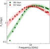 |
Fig. 5 Modelling of radio spectra on ∆t = 392 and 557 days according to the SN-CSM interaction model where inhomogeneities in the CSM are introduced through a magnetic-field probability distribution (Eq. (9)). Shaded lines are uniformly drawn parameters from the posteriors of the fitted parameters. |
5 Conclusions
In this paper, we present multi-epoch, broadband radio observations of the peculiar case of SN 2019oys. SN 2019oys was first classified as a Type Ib SN, but after ~100 days it showed optical rebrightening and a spectral transition to a spectrum mainly dominated by CSM interaction and a plethora of narrow, high-ionisation lines, including coronal lines. About 150 days after the re-brightening the optical light curve began to slowly fade, and since then it continued to decline.
Our broadband radio observations presented here, taken with the VLA and AMI-LA, show a bright radio source at late times, which is in agreement with the strong CSM interaction seen in the optical. Analysing the radio spectra on ∆t = 201 and 221 days has shown that the radio emission from a synchrotron self-absorbed source is accompanied by an FFA from the material in front of the shock. Initial analysis of the radio spectral peaks, not taking electron cooling into consideration, suggested magnetic fields of 1–2 G at a relatively late time after the explosion. In addition, the power-law index of the electron energy distribution was extremely high (p = 4.4 ± 0.4) for the spectrum obtained on ∆t = 221 days. Such a steep power-law index and high magnetic fields point towards electron cooling (either by synchrotron and/or IC cooling). We find that the synchrotron cooling frequency is lower than all of our observed frequencies on ∆t = 201 and 221 days, thus making it important for our analysis. We did not test for IC cooling as its frequency is highly dependent on the bolometric luminosity, which we do not know.
Taking synchrotron cooling into consideration, we find that the power-law index of the electron energy distribution is 3.4 ± 0.4 on ∆t = 221 days. Since we lack the coverage of high frequencies in the optically thin regime on ∆t = 201 days, we cannot constrain the power-law index, p, at that epoch, and we assume that it does not change between epochs. Using the spectral peak and assuming that the CSM was deposited by constant mass loss in steady winds from the progenitor massive star, we find that the mass-loss rate, as observed on ∆t = 201 and 221 days, is (1.0 ± 0.5) × 10−3 and (9.2 ± 0.6) ×10−4 M⊙ yr−1 (assuming wind velocity of 100 km s−1). This translates to a density of (4.1 ± 0.8) × 105 cm−3 at a distance of (2.6 ± 0.2) × 1016cm, which agrees with the CSM density of the region responsible for the narrow, high-ionisation lines seen in optical spectra (Sollerman et al. 2020).
The temporal evolution of SN 2019 oys is slowed down when compared to other Type Ib SNe. The 15.5 GHz light curve shows a slow decline of t−0.71±0.07, which is also slower than the t−1 expected in the scenario of a shock traveling with a constant velocity in a spherical, r−2, density structure (Chevalier 1998). Furthermore, the analysis above suggests a decelerating shock velocity of (1.1 ± 0.1) × 104 kms−1 on ∆t = 201 and 221 days and (0.8 ± 0.1) × 104 kms−1 on ∆t = 392 days. These values are lower than the velocities observed in radio for most Type Ib SNe. However, typically, velocities of Type Ib SNe are measured early on (within weeks of and up to a few months after the explosion), and the velocity of SN 2019oys was measured about seven months after optical discovery. Furthermore, Type IIn SNe are typically slowed down by the dense CSM surrounding the progenitor. Thus, it is possible that this low velocity is due to mass accumulation by the shock travelling in a dense CSM (which is also supported by the observed shock deceleration).
SN 2019oys also shows late-time radio spectra with unusually broad spectral peaks. These spectral peaks can be interpreted as a synchrotron-emitting source from a non-homogeneous CSM structure. We fitted a model describing the CSM inhomogeneities as arising from variations in the distribution of the relativistic electrons and/or the magnetic field strength; we did so by introducing a power-law distribution for the magnetic field strength as presented in Björnsson (2013); Björnsson & Keshavarzi (2017). This model manages to describe the data; however, due to the lack of spectral coverage we can only put upper limits on some of the model parameters. Better spectral coverage is needed to allow us to fully observe the transition from the broad spectral peak to the optically thick and thin regimes. This will provide improved constraints on the physical properties of the shock and its environment. Furthermore, probing the synchrotron spectrum of a spatially resolved source is a direct probe of the CSM structure at a given radius. Thus, future Very Long Baseline Interferometry (VLBI) observations of nearby CCSNe can resolve the structure of the emitting region and provide direct evidence for CSM inhomogeneities. Comparing the spectral peak broadness of SN 2019oys to other notable SNe shows that the CSM structure around the SN is highly non-homogeneous; however, broader peaks have been observed in several cases (e.g. PTF 11qcj; Corsi et al. 2014).
Overall, SN 2019oys shows strong CSM interaction at late times, both in the optical and radio. It shows significant signs of FFA absorption in the radio, implying a high density at a large distance and a non-homogeneous CSM structure. The evolution of the radio spectrum of SN 2019oys raises interesting questions as of the formation of the CSM structure encompassing its progenitor. For example, it is somewhat surprising that the outer regions (observed in the late-time radio spectra) are non-homogeneous, while the inner CSM (observed in the early radio spectra) points towards a rather homogeneous CSM shell (without a broad radio spectral peak). Such variations in the CSM structure over relatively short timescales prior to the SN explosion can be an indication of several distinct mass-loss episodes at the end of the massive star’s life. This is somewhat reminiscent of the optical signatures of extreme mass-loss episodes about a year prior to the explosion, which are sometimes seen in recombination emission lines via the technique of flash spectroscopy: rapid spectroscopic observations of SNe, shortly (hours) after they explode (Gal-Yam et al. 2014).
SN 2019oys demonstrates the importance of late-time observations of SNe in the optical and, especially, in the radio. Late-time radio observations play a key role in revealing the mass-loss history of massive stars in different epochs of their evolution.
Acknowledgements
We thank an anonymous referee for helpful comments. A.H. is grateful for the support by the Israel Science Foundation (ISF grant 1679/23) and by the United States-Israel Binational Science Foundation (BSF grant 2020203). We acknowledge the staff who operate and run the AMI-LA telescope at Lord’s Bridge, Cambridge, for the AMI-LA radio data. AMI is supported by the Universities of Cambridge and Oxford, and by the European Research Council under grant ERC-2012-StG-307215 LODESTONE. We thank the National Radio Astronomy Observatory (NRAO) for carrying out the Karl G. Jansky Very Large Array (VLA) observations. D.R.A.W was supported by the Oxford Centre for Astrophysical Surveys, which is funded through generous support from the Hintze Family Charitable Foundation. S. Schulze is partially supported by LBNL Subcontract No. 7707915 and by the G.R.E.A.T. research environment, funded by Vetenskapsrådet, the Swedish Research Council, project number 2016–06012. This research has made use of the CIRADA cutout service at cutouts.cirada.ca, operated by the Canadian Initiative for Radio Astronomy Data Analysis (CIRADA). CIRADA is funded by a grant from the Canada Foundation for Innovation 2017 Innovation Fund (Project 35999), as well as by the Provinces of Ontario, British Columbia, Alberta, Manitoba and Quebec, in collaboration with the National Research Council of Canada, the US National Radio Astronomy Observatory and Australia’s Commonwealth Scientific and Industrial Research Organisation. We have made extensive use of the data reduction software CASA (McMullin et al. 2007), REDUCE_DC (Perrott et al. 2013), and the PYTHON EMCEE (Foreman-Mackey et al. 2013) package.
Appendix A Tables
SN 2019oys: radio observations.
SN 2019oys: fitting spectrum on Δt = 201 and 221 days.
Appendix B Spectrum corner plots
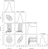 |
Fig. B.1 Posterior probability distributions from our MCMC analysis of radio spectrum obtained 392 days after discovery according to CSM inhomogeneities model introduced in Sect. 4 and in Björnsson (2013). The data clearly do not manage to constrain the upper value of the magnetic field distribution, B1, which is uniquely defined by the transition from the spectral peak to the optically thin regime. |
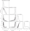 |
Fig. B.2 Posterior probability distributions from our MCMC analysis of radio spectrum obtained 557 days after discovery according to CSM inhomogeneities model introduced in Sect. 4 and in Björnsson (2013). The data do not manage to constrain the lower value of the magnetic field distribution, B0, which is uniquely defined by the transition from the optically thick regime to the spectral peak. |
References
- Anderson, G. E., Horesh, A., Mooley, K. P., et al. 2017, MNRAS, 466, 3648 [NASA ADS] [CrossRef] [Google Scholar]
- Barniol Duran, R., Nakar, E., & Piran, T. 2013, ApJ, 772, 78 [NASA ADS] [CrossRef] [Google Scholar]
- Bartel, N., Bietenholz, M. F., Rupen, M. P., et al. 2002, ApJ, 581, 404 [NASA ADS] [CrossRef] [Google Scholar]
- Bellm, E. C., Kulkarni, S. R., Barlow, T., et al. 2019, PASP, 131, 068003 [Google Scholar]
- Bietenholz, M. F., Bartel, N., Argo, M., et al. 2021, ApJ, 908, 75 [NASA ADS] [CrossRef] [Google Scholar]
- Björnsson, C. I. 2013, ApJ, 769, 65 [CrossRef] [Google Scholar]
- Björnsson, C. I., & Keshavarzi, S. T. 2017, ApJ, 841, 12 [CrossRef] [Google Scholar]
- Chandra, P., Nayana, A. J., Björnsson, C. I., et al. 2019, ApJ, 877, 79 [NASA ADS] [CrossRef] [Google Scholar]
- Chevalier, R. A. 1981, ApJ, 251, 259 [NASA ADS] [CrossRef] [Google Scholar]
- Chevalier, R. A. 1982, ApJ, 259, 302 [Google Scholar]
- Chevalier, R. A. 1998, ApJ, 499, 810 [NASA ADS] [CrossRef] [Google Scholar]
- Chevalier, R. A., & Fransson, C. 2006, ApJ, 651, 381 [NASA ADS] [CrossRef] [Google Scholar]
- Corsi, A., Ofek, E. O., Gal-Yam, A., et al. 2014, ApJ, 782, 42 [NASA ADS] [CrossRef] [Google Scholar]
- DeMarchi, L., Margutti, R., Dittman, J., et al. 2022, ApJ, 938, 84 [NASA ADS] [CrossRef] [Google Scholar]
- Filippenko, A. V. 1997, ARA&A, 35, 309 [NASA ADS] [CrossRef] [Google Scholar]
- Foreman-Mackey, D., Conley, A., Meierjurgen Farr, W., et al. 2013, Astrophysics Source Code Library [record ascl:1303.002] [Google Scholar]
- Gal-Yam, A. 2017, in Handbook of Supernovae, eds. A. W. Alsabti, & P. Murdin, 195 [CrossRef] [Google Scholar]
- Gal-Yam, A., Arcavi, I., Ofek, E. O., et al. 2014, Nature, 509, 471 [CrossRef] [Google Scholar]
- Graham, M. J., Kulkarni, S. R., Bellm, E. C., et al. 2019, PASP, 131, 078001 [Google Scholar]
- Hickish, J., Razavi-Ghods, N., Perrott, Y. C., et al. 2018, MNRAS, 475, 5677 [NASA ADS] [CrossRef] [Google Scholar]
- Horesh, A., Kulkarni, S. R., Fox, D. B., et al. 2012, ApJ, 746, 21 [NASA ADS] [CrossRef] [Google Scholar]
- Horesh, A., Stockdale, C., Fox, D. B., et al. 2013, MNRAS, 436, 1258 [NASA ADS] [CrossRef] [Google Scholar]
- Horesh, A., Sfaradi, I., Ergon, M., et al. 2020, ApJ, 903, 132 [NASA ADS] [CrossRef] [Google Scholar]
- Kamble, A., Margutti, R., Soderberg, A. M., et al. 2016, ApJ, 818, 111 [NASA ADS] [CrossRef] [Google Scholar]
- Lacy, M., Baum, S. A., Chandler, C. J., et al. 2020, PASP, 132, 035001 [Google Scholar]
- Langer, N. 2012, ARA&A, 50, 107 [CrossRef] [Google Scholar]
- McMullin, J. P., Waters, B., Schiebel, D., Young, W., & Golap, K. 2007, ASP Conf. Ser., 376, CASA Architecture and Applications, 127 [Google Scholar]
- Nayana, A. J., Chandra, P., & Ray, A. K. 2018, ApJ, 863, 163 [NASA ADS] [CrossRef] [Google Scholar]
- Perrott, Y. C., Scaife, A. M. M., Green, D. A., et al. 2013, MNRAS, 429, 3330 [NASA ADS] [CrossRef] [Google Scholar]
- Raftery, A. E. 1995, Sociol. Methodol., 25, 111 [CrossRef] [Google Scholar]
- Ruiz-Carmona, R., Sfaradi, I., & Horesh, A. 2022, A&A, 666, A82 [NASA ADS] [CrossRef] [EDP Sciences] [Google Scholar]
- Scott, M. A., & Readhead, A. C. S. 1977, MNRAS, 180, 539 [NASA ADS] [Google Scholar]
- Smith, N. 2014, ARA&A, 52, 487 [NASA ADS] [CrossRef] [Google Scholar]
- Soderberg, A. M., Kulkarni, S. R., Berger, E., et al. 2005, ApJ, 621, 908 [NASA ADS] [CrossRef] [Google Scholar]
- Soderberg, A. M., Chevalier, R. A., Kulkarni, S. R., & Frail, D. A. 2006, ApJ, 651, 1005 [CrossRef] [Google Scholar]
- Sollerman, J., Fransson, C., Barbarino, C., et al. 2020, A&A, 643, A79 [NASA ADS] [CrossRef] [EDP Sciences] [Google Scholar]
- Weiler, K. W., van Dyk, S. D., Panagia, N., Sramek, R. A., & Discenna, J. L. 1991, ApJ, 380, 161 [NASA ADS] [CrossRef] [Google Scholar]
- Weiler, K. W., Panagia, N., Montes, M. J., & Sramek, R. A. 2002, ARA&A, 40, 387 [NASA ADS] [CrossRef] [Google Scholar]
- Weiler, K. W., Williams, C. L., Panagia, N., et al. 2007, ApJ, 671, 1959 [NASA ADS] [CrossRef] [Google Scholar]
- Yadav, N., Ray, A., Chakraborti, S., et al. 2014, ApJ, 782, 30 [NASA ADS] [CrossRef] [Google Scholar]
- Zenati, Y., Wang, Q., Bobrick, A., et al. 2022, ApJ, submitted [arXiv:2207.07146] [Google Scholar]
- Zwart, J. T. L., Barker, R. W., Biddulph, P., et al. 2008, MNRAS, 391, 1545 [NASA ADS] [CrossRef] [Google Scholar]
We note that the assumption of a spherical, r–2, density profile arises from the assumption of a constant mass-loss rate from steady winds, which is not always true. In addition, the EM assumes a wide shell such that the integral of the electron density along the line of sight (Eq. (3)) does not depend on its width. If the interacting CSM shell is relatively thin and/or varies from the simple spherical density profile, as discussed later in Sect. 4, FFA optical depth may vary.
All Tables
All Figures
|
Fig. 1 Radio observations of SN 2019oys with VLA and AMI-LA (see Sect. 2). The left panel shows the broadband spectra obtained with the VLA in this work on four different epochs. The right panel shows the 15.5 GHz light curve obtained with AMI-LA (square markers) and the VLA (circle markers), and a 3 GHz light curve obtained by our VLA (circle markers) and VLASS (diamond marker) observations. The 3σ rms upper limits obtained by the VLA are marked with triangles. |
| In the text | |
|
Fig. 2 Modelling of radio spectra obtained by VLA on ∆t = 201 and 221 days after optical discovery. The left panel shows the fitting of Eq. (5) to the spectra, assuming SSA as the only absorption mechanism. The right panel shows the fitting of Eq. (5) multiplied by Eq. (6) to the spectra, assuming that the absorption is due to both SSA and FFA by the material in front of the shock. Both fits also show shaded lines uniformly drawn from the posteriors of the fitted parameters. |
| In the text | |
|
Fig. 3 Chevalier diagram of SN 2019oys (blue star marker for ∆t = 201 days and an orange star marker for ∆t = 221 days) with other Type Ib (grey circles) and IIn (grey squares) SNe. Also plotted for reference (green diamonds) are the two peaks observed in the 15.7 GHz light curve of SN 2014C (Anderson et al. 2017) which showed similar behaviour to SN 2019oys in the optical. The diagram shows the peak spectral radio luminosity, |
| In the text | |
|
Fig. 4 Modelling of 15.5 GHz light curve obtained with VLA and AMI-LA. The light curve was fitted with a two-power-law model. Shaded lines are uniformly drawn parameters from the posterior probability distributions of the fitted parameters. |
| In the text | |
|
Fig. 5 Modelling of radio spectra on ∆t = 392 and 557 days according to the SN-CSM interaction model where inhomogeneities in the CSM are introduced through a magnetic-field probability distribution (Eq. (9)). Shaded lines are uniformly drawn parameters from the posteriors of the fitted parameters. |
| In the text | |
|
Fig. B.1 Posterior probability distributions from our MCMC analysis of radio spectrum obtained 392 days after discovery according to CSM inhomogeneities model introduced in Sect. 4 and in Björnsson (2013). The data clearly do not manage to constrain the upper value of the magnetic field distribution, B1, which is uniquely defined by the transition from the spectral peak to the optically thin regime. |
| In the text | |
|
Fig. B.2 Posterior probability distributions from our MCMC analysis of radio spectrum obtained 557 days after discovery according to CSM inhomogeneities model introduced in Sect. 4 and in Björnsson (2013). The data do not manage to constrain the lower value of the magnetic field distribution, B0, which is uniquely defined by the transition from the optically thick regime to the spectral peak. |
| In the text | |
Current usage metrics show cumulative count of Article Views (full-text article views including HTML views, PDF and ePub downloads, according to the available data) and Abstracts Views on Vision4Press platform.
Data correspond to usage on the plateform after 2015. The current usage metrics is available 48-96 hours after online publication and is updated daily on week days.
Initial download of the metrics may take a while.