| Issue |
A&A
Volume 684, April 2024
|
|
|---|---|---|
| Article Number | A152 | |
| Number of page(s) | 6 | |
| Section | Planets and planetary systems | |
| DOI | https://doi.org/10.1051/0004-6361/202347859 | |
| Published online | 19 April 2024 | |
Mitigating stellar activity in radial velocity measurements through the spectral tracking of starspots
1
Department of Physics and Astronomy, Uppsala University,
Box 516,
75120
Uppsala, Sweden
e-mail: This email address is being protected from spambots. You need JavaScript enabled to view it.
2
Leiden Observatory, Leiden University,
Postbus 9513,
2300 RA
Leiden, The Netherlands
Received:
1
September
2023
Accepted:
11
January
2024
Abstract
Context. Extreme-precision radial velocity observations used to search for low-mass extrasolar planets are hampered by astrophysical noise originating from stellar photospheres. Starspots are a particular nuisance when observing young and active stars. New algorithms are needed to overcome the stellar noise barrier in radial velocity measurements.
Aims. Using simulations of stellar spectra, we aim to test a technique, which we call GUSTS, that directly measures the contribution from starspots by using spectral features that are distinct from the rest of the stellar photosphere. Their contributions are expected to be anti-correlated with the starspot-induced radial velocity jitter of the star. This is reminiscent of high-dispersion observations of a transiting planet, which causes a Rossiter-McLaughlin effect but also leaves an atmospheric transmission signature that, in the case of spin-orbital alignment, is anti-correlated in radial velocity with the Rossiter-McLaughlin effect.
Methods. We simulated rotating stars with a single starspot to test the method. Synthetic spectral time series were averaged to obtain a virtual spot-free star spectrum. The individual spectra were subsequently convolved with a kernel, using single value decomposition, to match the average spectrum as closely as possible, after which this average spectrum was removed from the individual spectra. The residual spectra were subsequently searched for spot signatures using the template spot spectrum used to make the synthetic stars. We tested this method on a variety of spectra with different signal-to-noise ratios and investigated what data quality is needed to use this technique in practice.
Results. We demonstrate that the new GUSTS technique can work to reduce radial velocity jitter from starspots given a highly sampled, high S/N dataset. Though this alone cannot take radial velocity jitter down to the level to see Earth-like planets, it can be combined with other methods and can be used on starspot-dominated stars to detect smaller and farther planets. This technique could be useful for the future Terra Hunting Experiment, which will provide high S/N data with large samples.
Key words: methods: data analysis / techniques: radial velocities / stars: activity
© The Authors 2024
 Open Access article, published by EDP Sciences, under the terms of the Creative Commons Attribution License (https://creativecommons.org/licenses/by/4.0), which permits unrestricted use, distribution, and reproduction in any medium, provided the original work is properly cited.
This article is published in open access under the Subscribe to Open model. This email address is being protected from spambots. You need JavaScript enabled to view it. to support open access publication.
1 Introduction
The radial velocity (RV) technique, one of the main ways to detect exoplanets, works by indirectly detecting the presence of an exoplanet via its gravitational pull on the host star. Instrumental precision and the long-term stability of spectrographs have made enormous leaps forward since the first discovery of a planet around a main sequence star (Mayor & Queloz 1995). Current generations of high-precision planet-hunting spectrographs, such as the High Accuracy Radial velocity Planet Searcher (HARPS; Pepe et al. 2002) and the Echelle SPectrograph for Rocky Exoplanet and Stable Spectroscopic Observations (ESPRESSO; González Hernández et al. 2018), reach an instrumental stability firmly in the sub-metre regime. Unfortunately, at this level astrophysical noise from the stellar photosphere starts to dominate even for the quietest stars, which obscures planetary signals and prevents observers from reaching the precisions necessary to detect Earth analogues. This astrophysical noise originates from various facets of the stars we observe, for example solar-type oscillations on a few-minute timescale (Claverie et al. 1979), starspots and plages rotating in and out of view that break the symmetry of stellar absorption lines (Hatzes 1999), long-term magnetic cycles that affect the RV signatures due to changes in convection suppression (Meunier et al. 2010), and granulation and supergranulation effects.
Many techniques and algorithms aimed at mitigating these stellar noise signals are under development, and many show promising results. Some current methods aim to measure precise RVs on individual spectral lines (Dumusque 2018; Cretignier et al. 2020; Al Moulla et al. 2022) or use joint photometric and RV measurements (Oshagh et al. 2017). Recently, data from the Extreme Precision Spectrograph (EXPRES) were used as part of the EXPRES Stellar-Signals Project (ESSP) to compare 22 different methods and test to what extent they reduce the RV RMS (Zhao et al. 2022), though no method was found to consistently work well enough. Activity indices such as the Ca II H&K lines are used to measure the activity levels of stars (e.g. Queloz et al. 2001). Zeeman Doppler imaging can determine the topology of surface magnetic fields in stars and provide insight into the distribution of cool spots using spectropolarimetric data (Rosén et al. 2015; Hackman et al. 2016). More recently, neural networks using Gaussian processes have attempted to model stellar activity signals in RV data (Rajpaul et al. 2015). Another complimentary avenue is to optimize the window function of RV measurements; this is the primary way the Terra Hunting Experiment (THE) aims to find Earth-twins (Thompson et al. 2016; Hall et al. 2018). Each method aims to tackle one or more aspects of the stellar activity problem, and many fully developed methods will be used together in upcoming RV surveys in order to hunt for true Earth twins.
In this paper, we present a method that focuses on mitigating stellar RV jitter from starspots. It uses evaluations of the unique spectral features of the spots themselves and their Doppler velocity induced by stellar rotation to determine their effect on RV measurements of the star. We name this technique GUSTS, which stands for the Global Unresolved Spectral Tracking of Starspots.
GUSTS combines various methods currently used to characterize exoplanet atmospheres, such as molecular band modeling, to measure starspot coverage and temperatures (Neff et al. 1995; O’Neal et al. 1998; Morris et al. 2019, 2020). In both the exo-planet transit and starspot cases, a dark feature transits across the stellar disk, leaving a characteristic Doppler shadow. This in turn leaves a distinct impression in the form of the Rossiter-McLaughlin effect, often used in the confirmation of exoplanets (see, as an example, Dorval et al. 2020), and also influences the RVs of the star. GUSTS uses similar initial steps but instead probes the influence of the dark spot on the measured stellar RV.
In Sect. 2, we discuss the method in detail. Section 3 presents our simulations and the reduction method. Section 4 presents our results, which are discussed further in Sect. 5.
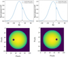 |
Fig. 1 Heavily exaggerated example of how starspots impact the CCF. Their lower flux leads to less contribution at certain velocities, depending on the position of the starspot on the stellar disk. |
2 Principle of the method: The global unresolved spectral tracking of starspots
All stars spin, which causes their observed absorption lines to be rotationally broadened proportional to v sin i, where v is the equatorial rotational velocity and i is the inclination of the star. In principle, rotational broadening is symmetric and does not change the overall RV of the star, although RVs of fast-rotating stars are more difficult to measure due to their significant spectral line broadening.
However, when starspots are present, the line symmetry is broken. These darker spots contribute much less to the overall flux of the star compared to unspotted areas, which results in small dents in the line profile, as shown heavily exaggerated in Fig. 1. This results in small measured blueshifts or redshifts, that is to say, RV jitter. This jitter from starspots or their brighter counterparts – plages – can contribute m s−1 to hundreds of m s−1 variations in more active stars (Hatzes 2002). The GUSTS method uses measurements of the spectral signature of spots to determine the global contributions of spots on the stellar disk; their impact on the stellar RV lines, such as from TiO, is not present in the spectra of solar-type stars, except in the significantly cooler starspot regions. By targeting these spot-specific lines, the overall contribution of the starspot to the average line profile (which depends on its location on the stellar surface) can be indirectly measured, and its impact on RV derived.
GUSTS uses a series of high signal-to-noise ratio (S/N) spectra that are well distributed over multiple stellar rotation periods. In this paper, a set of simulations is constructed to mimic what would be needed observationally. These simulations include a stellar surface similar to that of e Eridani with a starspot in random positions along the equatorial plane of the star with a lower temperature – either 500 or 1000 K below that of the rest of the star.
The non-starspot stellar features in this data are removed in a way analogous to how stellar information is removed when characterizing exoplanet atmospheres through the use of singular value decomposition (SVD) or principle component analysis. The use of SVD removes normal photospheric lines from data, leaving only the unique starspot signatures. Subsequently, cross-correlation to a theoretical starspot template yields a function that, when integrated, provides a measure of the starspot distribution at the time of observation. With sufficient data, these measures can be compared with the stellar RVs. Linearly fitting these data mitigates RV jitter resulting from the impact of starspots. This is discussed further in Sect. 5.
3 GUSTS simulations
The simulations we carried out to assess the performance of GUSTS in reducing the RV jitter from starspots consisted of three parts: the first was the initial preparation, which consisted of constructing the spectral templates and injecting noise to simulate observations. The second was analysing GUSTS to determine the RV impact of the spots and their anti-correlation to stellar RVs. The third was an analysis to determine the quality of observational data required for GUSTS to be effective. These steps are described in the following subsections.
3.1 Constructing simulated spectra
A set of mock observations was constructed to test GUSTS. A stellar disk was modelled using a binary mask with a radius of 40 pixels, multiplied by a linear limb-darkening law given by Eq. (1), where a is the radius of the stellar disk, r is the radial distance from the centre, and u is the limb-darkening coefficient, assumed to be 0.55:
![Mathematical equation: $I(r) = I(0)\,\left[ {1 - u\,\left( {1 - \sqrt {{{{a^2} - {r^2}} \over {{a^2}}}} } \right)} \right].$](/articles/aa/full_html/2024/04/aa47859-23/aa47859-23-eq1.png) (1)
(1)
The model star was given a rotational velocity of 25 km s−1, corresponding to a young active star, and a starspot with a range of phases was injected. The spot was placed in 64 positions, regularly spread out along the equator as it was determined that the longitudinal placement would only effect later results to the second order. The spot size was set to be either 5% or 10% of the size of the star, corresponding to an area of 1 or 0.25% of the observed stellar disk, which we classified as a ‘small’ or ‘large’ spot, respectively. The spots were also chosen to have a temperature of either 3600 or 4500 K and classified as ‘cool’ or ‘warm’. As such, four different starspot models were used and tested: a small cool spot, a large cool spot, a small warm spot, and a large warm spot. This was done to measure the influence of the temperature and size of the spots on the GUSTS analysis.
Each pixel on the stellar surface was designated to belong to either a starspot or a star pixel, and a matching Coelho synthetic spectrum (Coelho 2014) was injected in each pixel with a Doppler-shifted velocity that matched the RV component towards an observer. The spectra had a wavelength range of 380–690 nm to match the wavelength range of a HARPS-like instrument. The spectra of all pixels were then summed, wavelength-interpolated, and convolved to match the resolution of HARPS (R = 115 000). The relevant parameters for the synthetic spectra are given in Table 1.
Parameters used for extracting the spectral templates from Coelho (2014).
3.2 Reducing stellar contributions to simulations
As described above, each simulated observation is composed of a large number of stellar pixels and a few starspot pixels, depending on the phase of the spot and whether the spot is on the observed side of the stellar surface. As in real observations, the integrated spectrum is completely dominated by the light coming from the normal photosphere. This needs to be removed first to enable the detection of spectral features of the starspots. For this, we first constructed a master reference. An assumption is made that, given enough observations, the median spectrum of a time series of a star will not contain significant information about transient phenomena and will be close to the spectrum of the star when it has no spots. In other words, as a starspot is not a permanent fixture on a stellar disk and changes position over time, it should only be present at that velocity position for a minority of the observations and thus can be removed by taking a median of all observations. This is only true if a sufficient number of observations have been taken spread out over enough time. We call this median spectrum the master reference.
Subsequently, we used SVD with the master reference to alter the line-spread function of each individual spectra to fit the stellar spectrum as well as possible. SVD takes each spectrum and finds a kernel that, when convolved with this spectrum, fits the master reference best. This means that the normal photospheric lines of the star are optimally matched to the reference while leaving the unique starspot features relatively unchanged. This we call the SVD-corrected spectra, in which the common spectral lines in the different observations are of similar amplitude, position, shape, and width, with any unique features being slightly broadened and slightly shifted. Following this, the master reference is divided out of all observations, which strongly reduces spectral features from the main photosphere. A mask was applied to set regions where one would expect tellurics in real observations. A mask was also applied to regions with large simulated abnormalities coming from edge reductions carried out using SVD to the continuum. The masked regions account for less than one percent of the spectrum.
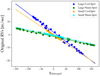 |
Fig. 2 Comparison of four noiseless simulations: small or large spots that are warm or cool. Only the temperature of the spot influences the slope of the measured stellar RV versus ηspot. |
3.3 Characterizing the spot through cross-correlation
As described above, the simulations now have minor features from the main photosphere, with the unique starspot features still present in the spectra. The next step involves cross-correlating each simulated observation to different templates. Three separate cross-correlations are performed. The first cross-correlation is between the original, non-SVD-corrected spectra and the star template of 5000 K to determine the nominal RV. The second cross-correlation is between the SVD-corrected spectra and the same star template. This is used as an indication of how well the SVD correction reduces the main photospheric features in the spectra. The last cross-correlation is between the SVD-corrected data and the starspot templates. All cross-correlation functions (CCFs) were individually normalized.
3.4 Recovering starspot effects on radial velocity
These CCFs contain all the information needed to understand the spot effects on the original RVs. An integral is taken of the starspot CCFs and is multiplied by the velocity shifts  , referred to as ηspot) within the velocity limits set by the stellar rotation (25 km s−1) as a measure of the weighted mean of starspot impact. This integral contains information on the latitudinal position of the spot, or the weighted mean if more than one spot is present. If a starspot is in the blueshifted region, the integral of the starspot CCF will peak at negative velocities, and thus ηspot will be more negative. For a starspot in the red-shifted region, the opposite is true since the starspot CCF will peak at positive velocities. One can extrapolate this to understand how multiple starspots will impact this integral. If the majority of starspots are in the blueshifted region, the integral will be negative. If the majority of starspots are in the redshifted region, the integral will be positive.
This integral is then compared to the measured RVs of the original spectra for all observations. A linear fit is performed to quantify how the starspot activity affected the RV measurements. This fit is then subtracted from the original RVs to calculate the reduced RVs.
3.5 Required quality of observational data
The four starspot models (small cool spot, large cool spot, small warm spot, and large warm spot) were simulated to determine the amount and quality of observational data required to obtain a significant reduction in stellar RV jitter from starspots. A set of 340 simulations was constructed as described above, after which a random sample was taken. We chose 5, 10, 50, 100, or 200 observations to represent the number of observations on a target. Gaussian noise was introduced in the modelled spectra to simulate S/Ns of 100, 300, 400, and 500. This analysis was repeated 500 times for each random sampling number to determine how the number of observations effects the RV accuracy, with the standard deviation of the 500 realisations taken as the uncertainty.
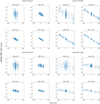 |
Fig. 3 Comparison of four different simulations with different S/Ns – 100, 300, 500, or 1000 – with the four different spot templates – cool or warm and small or large – and their effects on RV. For readability purposes, the x scale for the large warm spot is increased by a factor of two. |
4 Results
This technique was assessed using simulations of four different starspots (warm or cool and small or large). The relationship between the stellar RVs and the spot integrals is presented in Fig. 2 for a noise-free case to show how the temperature and size of a spot change this relationship: only the temperature of the spot influences the slope, not the spot size.
Adding different levels of noise to the simulations gives an indication of the amount and quality of observational data needed for GUSTS to work well. Figure 3 show the different effects of assumed S/Ns on the four different spot templates. In these diagrams there are clumps of data located in a vertical line where ηspot ≈ 0, which come from the times that the spot is not visible to the observer. They come from simulated data where the phase position of the spot places it behind the star. In these cases, the RV jitter comes solely from the noise, and a cross-correlation to the starspot template shows no signal.
By taking random samples of the data and reducing the linear fit, we determined the reduction in RV jitter as a function of the number and quality (S/N) of observations. Figure 4 shows the reduction in RV jitter from starspots (in percent) compared to the number of data points used to reduce the data for S/Ns of 100, 300, 400, 500, and 1000.
The reduction in RV jitter from starspots is heavily dependent on the S/N of observations, as well as the size and temperature of the spot. For smaller spots, one can expect a reduction in RV jitter of a few percent to greater than 10% for warmer or cooler spots; that is, if spots cause a 5 m s−1 jitter, a GUSTS analysis on 25 data points with a S/N of 300 could reduce the jitter to 4.25 m s−1 for cooler spots. For larger spots, this reduction is more prominent. For a cool spot twice the radius of the previous, leading to a 20 m s−1 jitter, a GUSTS analysis on similar data could reduce the RV jitter by around 60 percent, reducing the starspot jitter from 20 m s−1 to 8 m s−1.
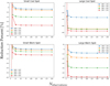 |
Fig. 4 Comparing the reduction in starspot RV noise for various spot sizes and temperatures. This is done across S/Ns of 100, 300, 400, and 500. An additional S/N of 1000 is used for the small warm spot as the lower-quality simulations do not reduce the RV signal significantly. It is important to note that a negative RV reduction here signifies a decrease in RV jitter, whereas a positive RV reduction signifies an increase in RV jitter. |
5 Discussion and conclusion
An important result is that the relation between the measured stellar RV and ηspot is nearly perfectly linear, meaning that a GUSTS analysis is valid for any combination of spots provided they have the same temperature. As shown in Fig. 2, the smaller the spot and the smaller the temperature difference between the spot and the star, the higher the S/N needs to be to lead to a significant reduction in RV. This is mitigated by the fact that these smaller spots have a smaller RV jitter effect to begin with. In a perfect case, a small warm spot producing a 1 m s−1 jitter can have its RV jitter reduced to 0.9 m s−1. A star with such starspots would not be the best case for a GUSTS analysis. However, a starspot with double the radius and the same temperature would produce a 4 m s−1 jitter, which would be reduced to around 1.6 m s−1 in the best case, a significant improvement. This is heightened for cooler spots, where a small spot could have its RV jitter reduced from 5 m s−1 to 3.25 m s−1, and a larger spot could have its RV jitter reduced from 20 ms−1 to 3 m s−1. These calculations were done assuming 50 or more observations with a S/N of 500.
In these simulations, the smallest spot is still quite large compared to realistic single spots, with a radius of around 5% of the stellar radius, which is around 0.25% of the stellar disk seen by an observer. This is similar to the size of some of the largest sunspots observed on the Sun, but is larger than average observed sunspots. Starspot contributions can be linearly added, so two small spots close to one another can act as one larger starspot. For these kinds of cool spots, we would still need at least a S/N of 300 with at least 25 observations, preferably 50, in order to have a chance at using this technique, though this depends on the spot distribution. For warmer spots, this becomes much more difficult. If a star has few starspots or very small starspots, such as the case of the Sun during low activity periods (i.e. with very low RV jitter from starspots), this step will require observations with S/Ns of greater than 500, and the RV reduction efficiency will be extremely small. As such, a GUSTS analysis is better suited for stars with large distributions of starspots, where the reduction efficiency is significant.
As expected, the temperature and size of the starspots have large effects on the RV noise and subsequently on the fraction that can be reduced. One spot whose radius is double that of a second can have RV effects close to four times higher, but may also have signals that, as seen with this technique, are close to four times larger as well. Similarly, warmer starspots have less of an RV effect due to the closer spectra and more similar intensities, but their signals are clearer when the ηspot is calculated.
It is clear that high-quality data are needed to use this technique. An observer would realistically need 50 or more observations of data with S/Ns of 400 or more for most semi-active stars. However, for stars with larger and cooler starspots, an observer might need only 25 observations with S/Ns of 300 or higher to get a significant improvement in jitter removal. This technique is better suited for stars with larger and cooler starspots with longer rotation periods. It is important to note that for these simulations the spot model is only a basic approximation of what a real spot would look like on the surface of a star. These simulations do not take more complicated starspot effects into consideration, such as their ability to suppress convective blueshift in spectral data or any other magnetic field effects. As such, the observational data needed to use this technique should be taken as an optimistic lower limit.
GUSTS seems to help reduce RV jitter due to starspots. However, there are two challenges in applying the method to real data: an observer would need extremely high-S/N data, such as from higher-magnitude stars (Vmag < 8) observed with ESPRESSO, and have an extremely well-sampled set of data (ndata > 50). The dataset needed must come from an observation platform such as the future THE. As such, applications of this technique to real data are currently limited.
In any case, GUSTS is a useful technique that offers a way to correct for noise that was previously left in RV surveys, provided the data have sufficiently high S/Ns and are extremely well sampled. This offers the possibility to lower the RV jitter floor of more active, starspot-dominated stars. GUSTS works best when used for younger, faster-rotating stars, when it can take advantage of the star’s dependence on spot distribution, size, and temperature; in these cases, it should work in conjunction with other techniques. Real-world application of GUSTS is limited due to the need for extremely high-S/N data with a high time-sampling of observations. In future work, we will test this method against different stars of varying activity levels and spectral type and use suitable archival data. This data will be used in conjunction with other similar techniques, such as measuring line bisectors or using the skew normal distribution of the CCF for comparison (see Simola et al. 2022). In order to fully judge how well this method reduces the observed starspot activity, it must also be applied to high-S/N, highly sampled data taken in conjunction with spectropolarimetric observations and used for Doppler imaging on stars with spots to compare the RV reduction with true, characterized starspots.
References
- Al Moulla, K., Dumusque, X., Cretignier, M., Zhao, Y., & Valenti, J. A. 2022, A&A, 664, A34 [NASA ADS] [CrossRef] [EDP Sciences] [Google Scholar]
- Claverie, A., Isaak, G., McLeod, C., van der Raay, H., Cortés, T. R. 1979, Nature, 282, 591 [NASA ADS] [CrossRef] [Google Scholar]
- Coelho, P. R. T. 2014, MNRAS, 440, 1027 [Google Scholar]
- Cretignier, M., Dumusque, X., Allart, R., Pepe, F., & Lovis, C. 2020, A&A, 633, A76 [NASA ADS] [CrossRef] [EDP Sciences] [Google Scholar]
- Dorval, P., Talens, G. J. J., Otten, G. P. P. L., et al. 2020, A&A, 635, A60 [NASA ADS] [CrossRef] [EDP Sciences] [Google Scholar]
- Dumusque, X. 2018, A&A, 620, A47 [NASA ADS] [CrossRef] [EDP Sciences] [Google Scholar]
- Gonzalez Hernandez, J. I., Pepe, F., Molaro, P., & Santos, N. C. 2018, ESPRESSO on VLT: An Instrument for Exoplanet Research, 157 [Google Scholar]
- Hackman, T., Lehtinen, J., Rosén, L., Kochukhov, O., & Käpylä, M. J. 2016, A&A, 587, A28 [NASA ADS] [CrossRef] [EDP Sciences] [Google Scholar]
- Hall, R. D., Thompson, S. J., Handley, W., & Queloz, D. 2018, MNRAS, 479, 2968 [NASA ADS] [CrossRef] [Google Scholar]
- Hatzes, A. 2002, Astron. Nachr., 323, 392 [NASA ADS] [CrossRef] [Google Scholar]
- Hatzes, A. P. 1999, in Precise Stellar Radial Velocities, eds. J. B. Hearnshaw, & C. D. Scarfe, Astronomical Society of the Pacific Conference Series, 185, IAU Colloq. 170: 259 [NASA ADS] [Google Scholar]
- Mayor, M., & Queloz, D. 1995, Nature, 378, 355 [Google Scholar]
- Meunier, N., Desort, M., & Lagrange, A. M. 2010, A&A, 512, A39 [NASA ADS] [CrossRef] [EDP Sciences] [Google Scholar]
- Morris, B. M., Curtis, J. L., Sakari, C., Hawley, S. L., & Agol, E. 2019, AJ, 158, 101 [NASA ADS] [CrossRef] [Google Scholar]
- Morris, B. M., Hoeijmakers, H. J., Kitzmann, D., & Demory, B.-O. 2020, AJ, 160, 5 [NASA ADS] [CrossRef] [Google Scholar]
- Neff, J. E., O’Neal, D., & Saar, S. H. 1995, ApJ, 452, 879 [NASA ADS] [CrossRef] [Google Scholar]
- O’Neal, D., Neff, J. E., & Saar, S. H. 1998, ApJ, 507, 919 [CrossRef] [Google Scholar]
- Oshagh, M., Santos, N. C., Figueira, P., et al. 2017, A&A, 606, A107 [NASA ADS] [CrossRef] [EDP Sciences] [Google Scholar]
- Pepe, F., Mayor, M., Rupprecht, G., et al. 2002, The Messenger, 110, 9 [NASA ADS] [Google Scholar]
- Queloz, D., Mayor, M., Udry, S., et al. 2001, The Messenger, 105, 1 [NASA ADS] [Google Scholar]
- Rajpaul, V., Aigrain, S., Osborne, M. A., Reece, S., & Roberts, S. 2015, MNRAS, 452, 2269 [Google Scholar]
- Rosén, L., Kochukhov, O., & Wade, G. A. 2015, ApJ, 805, 169 [Google Scholar]
- Simola, U., Bonfanti, A., Dumusque, X., et al. 2022, A&A, 664, A127 [NASA ADS] [CrossRef] [EDP Sciences] [Google Scholar]
- Thompson, S. J., Queloz, D., Baraffe, I., et al. 2016, SPIE Conf. Ser., 9908, 99086F [Google Scholar]
- Zhao, L. L., Fischer, D. A., Ford, E. B., et al. 2022, AJ, 163, 171 [NASA ADS] [CrossRef] [Google Scholar]
All Tables
All Figures
|
Fig. 1 Heavily exaggerated example of how starspots impact the CCF. Their lower flux leads to less contribution at certain velocities, depending on the position of the starspot on the stellar disk. |
| In the text | |
|
Fig. 2 Comparison of four noiseless simulations: small or large spots that are warm or cool. Only the temperature of the spot influences the slope of the measured stellar RV versus ηspot. |
| In the text | |
|
Fig. 3 Comparison of four different simulations with different S/Ns – 100, 300, 500, or 1000 – with the four different spot templates – cool or warm and small or large – and their effects on RV. For readability purposes, the x scale for the large warm spot is increased by a factor of two. |
| In the text | |
|
Fig. 4 Comparing the reduction in starspot RV noise for various spot sizes and temperatures. This is done across S/Ns of 100, 300, 400, and 500. An additional S/N of 1000 is used for the small warm spot as the lower-quality simulations do not reduce the RV signal significantly. It is important to note that a negative RV reduction here signifies a decrease in RV jitter, whereas a positive RV reduction signifies an increase in RV jitter. |
| In the text | |
Current usage metrics show cumulative count of Article Views (full-text article views including HTML views, PDF and ePub downloads, according to the available data) and Abstracts Views on Vision4Press platform.
Data correspond to usage on the plateform after 2015. The current usage metrics is available 48-96 hours after online publication and is updated daily on week days.
Initial download of the metrics may take a while.