© The Authors 2024

1. Introduction

Upon their discovery of buckminsterfullerene (C₆₀), Kroto et al. (1985) noted that its stability would allow this molecule to survive in space, and pointed out its potentially important role in interstellar chemistry of allowing reactions to be catalysed on its surface. Kroto & Jura (1992) had previously suggested C₆₀ could be a carrier of the mysterious diffuse interstellar bands (DIBs), a set of roughly 600 unidentified spectral absorption features seen to originate ubiquitously from interstellar material (Heger 1922; Merrill 1934; Herbig 1995; Tielens & Snow 1995; Cox & Cami 2014; Cox et al. 2017). The buckminsterfullerene cation (${\text{C}}_{\text{60}}^{\text{+}}$) was the first, and is so far the only, molecule with electronic transitions shown to match several DIBs (Foing & Ehrenfreund 1994, 1997; Campbell et al. 2015; Walker et al. 2015, 2016; Spieler et al. 2017; Linnartz et al. 2020). Neutral C₆₀ and C₇₀ have also been observed towards planetary nebulae such as TC1 Cami et al. (2010).

The association of the λ9577 and λ9632 DIBs with ${\text{C}}_{\text{60}}^{\text{+}}$ as their carrier has made it conceivable that related compounds, such as hydrogenated and metallofullerenes, exist in the diffuse interstellar medium (ISM), suggesting that there may be DIBs that originate from derivatives of C₆₀ and other fullerene cages. However, the identification of DIBs with their carrier species requires the comparison of laboratory gas-phase spectra to interstellar spectra, and these laboratory spectra are rarely available and difficult to obtain. In order to narrow the search for DIB carrier molecules, we can model environmental dependences and the stability of candidate carriers. The present work aims to model steady-state fullerene hydrogenation chemistry in order to understand whether it would be feasible to look for the spectral signatures of hydrogenated fullerenes.

Both polycyclic aromatic hydrocarbons (PAHs) and fullerenes can be (de-)hydrogenated to different degrees. Vuong & Foing (2000) provide a theoretical framework for understanding which of the different hydrogenation states of PAHs are more relevant in interstellar chemistry. Four chemical processes in the ISM were considered: photo-dissociation, photo-ionisation, electronic recombination, and reactions between PAH cations and H or H₂ (see e.g. Le Page et al. 2001; Jolibois et al. 2005; Montillaud et al. 2013; Castellanos et al. 2018 for studies on the hydrogenation states of PAHs). Fullerene cages C₆₀ and C₇₀ are known to react with hydrogen to form hydrogenated fullerenes (fulleranes) under certain laboratory conditions (Schröder et al. 1992; Brühwiler et al. 1993; Leidlmair et al. 2011; Kaiser et al. 2013; Cataldo et al. 2014). Recent reviews of interstellar fulleranes are available in Omont (2016) and Zhang et al. (2020). As with the hydrogenation of PAHs (Vuong & Foing 2000), the abundance of fulleranes is expected to be governed by the balance between the hydrogen abundance, which favours hydrogenation rates, and the UV flux, which favours de-hydrogenation.

2. Environmental parameters and assumptions

Because we aim to characterise how the hydrogenation chemistry depends on environmental parameters, it is important to first outline the type of environment we considered. In this section, we briefly describe diffuse cloud environments, and state the assumptions regarding environmental parameters underlying our model. These assumptions concern the main environmental characteristics that govern the hydrogenation chemistry: the density of atomic hydrogen and the UV photon flux. To model the ionisation state, we must furthermore consider the electron density.

Hydrogen density in diffuse clouds typically ranges from ten to several hundred atoms per cubic centimetre (Snow & McCall 2006). Hydrogen in diffuse clouds exists mostly in atomic form, and makes a sharp transition to molecular form with increasing cloud depth. We assumed that the UV photon flux can be characterised by the Draine field, multiplied by some factor ([ϕ]< 1) to account for extinction inside the cloud. Electron density is mostly determined by the carbon abundance in the regions where all carbon is ionised. Following Le Page et al. (2001), we assumed the electron density to be a constant fraction of the atomic hydrogen density. Le Page et al. (2001) took the value of this fraction to equal a previously determined C/H ratio of 1.4 × 10⁻⁴. We chose to follow Bakes & Tielens (1995) and started by assuming an electron-to-hydrogen ratio of 7.5 × 10⁻³. We then investigated how these different values influence the model outcomes. For the temperature, we assumed a constant value of 100 K.

Considering that the hydrogen density is substantially larger than that of carbon, we assumed that reactions between C₆₀ and hydrogen occur on a much shorter timescale than reactions with carbon that alter the bare cage structure. This means that the fullerenes have time to reach an equilibrium distribution of hydrogenation state before its carbon structure is altered, allowing us to model the hydrogenation state of C₆₀ according to a steady state balance while leaving cage growth and fragmentation processes out of consideration.

3. Competing reactions and rate coefficient estimation

Predicting the abundance of any molecule in interstellar clouds requires a detailed understanding of its destruction and formation mechanisms, how these mechanisms depend on the environment, and at what timescale each process occurs. To estimate the hydrogenation state of fullerenes in interstellar clouds, the first step is thus to identify and characterise the chemical reactions leading to hydrogenation and de-hydrogenation of fullerene cages. As outlined in the previous section, our model relies on a number of approximations regarding environmental parameters. In order to describe the charge and hydrogenation states of C₆₀, we furthermore assumed that the balance is regulated through the accretion of hydrogen onto neutral or charged fullerene cages, the removal of hydrogen through photo-dissociation, electron attachment or recombination, and electron photo-detachment. We thus assumed that we could neglect any other mechanisms such as interactions with H⁺ and ${\text{H}}_3^{\text{+}}$, charge transfer reactions, and associative detachment. The expected consequences of these simplifications are discussed in Sect. 3.8.

In the following sections, we discuss the main formation and destruction routes for hydrogenated C₆₀ in the neutral and cationic charge states. For each reaction, we combined reports from the literature with computations to quantify a corresponding rate coefficient. The reactions and rate coefficients in question are summarised in Table 1, along with the assumptions used to obtain rate values.

3.1. Hydrogen accretion onto neutral C₆₀

Hydrogenated C₆₀ is formed by the accretion of hydrogen onto the fullerene cage and subsequent radiative stabilisation:

$$\begin{array}{c}\hfill {\mathrm{C}}_{60}{\mathrm{H}}_i+\mathrm{H}\to {\mathrm{C}}_{60}{\mathrm{H}}_{i+1}+\varphi ,\end{array}$$(1)

where ϕ represents the radiation of excess energy after bond formation. The accretion of two hydrogen atoms during a collision with molecular hydrogen is also possible, but requires the dissociation of the hydrogen molecule. This introduces an energy barrier of ∼4 eV (Vehviläinen et al. 2011), leading us to neglect this process.

Hydrogen atoms can bind to the C₆₀ molecule upon collision without a barrier (Vehviläinen et al. 2011). The bond formation produces an excess energy of roughly 2 eV (Bettinger et al. 2002; Vehviläinen et al. 2011), which must be radiated away vibrationally in order for the bond to stabilise. Based on the analysis of radiative association for large molecules by Herbst & Dunbar (1991), we assumed that the radiative association of hydrogen to C₆₀ proceeds at the collisional rate for all hydrogenation states, i.

For a gas-phase reaction between two species A and B, the reaction rate r(T) as a function of the temperature T can be described as follows:

$$\begin{array}{c}\hfill r(T)=k{n}_A{n}_B=Z\rho exp(\frac{-E_{\mathrm{A}}}{\mathit{RT}}),\end{array}$$(2)

where k is the reaction rate coefficient in cm³ s⁻¹, n_A and n_B are the abundances of A and B in cm⁻³, Z is the frequency of collisions in cm³ s⁻¹, ρ is the fraction of collisions that results in a reaction (also called the steric factor), E_A is the activation energy of the reaction, and R is the gas constant. As we are considering a barrier-less reaction, we set E_A = 0 and, working under the assumption that a reaction occurs at each collision, we took ρ = 1. The collision frequency, Z, can be approximated using the hard-sphere model:

$$\begin{array}{c}\hfill Z=n_A{n}_B{\sigma }_{\mathit{AB}}\sqrt{\frac{8k_{B}T}{\pi {\mu }_{\mathit{AB}}}},\end{array}$$(3)

where the cross-section can be approximated as σ_AB = π(r_A + r_B)² with r_A and r_B the radii of the reactants A and B, k_B is the Boltzmann constant, and μ_AB = m_Am_B/(m_A + m_B) is the reduced mass of the reactants. The reaction rate coefficient can now be written as

$$\begin{array}{cc}\hfill k& ={\sigma }_{\mathit{AB}}\sqrt{\frac{8k_{\mathrm{B}}T}{\pi {\mu }_{\mathit{AB}}}},\hfill \end{array}$$(4)

$$\begin{array}{cc}& ={(r_A+r_B)}^2\sqrt{\frac{8\pi k_{\mathrm{B}}T(m_A+m_B)}{m_A{m}_B}},\hfill \end{array}$$(5)

$$\begin{array}{cc}& \approx {(r_A+r_B)}^2\sqrt{\frac{8\pi k_{\mathrm{B}}T}{m_B}},\hfill \end{array}$$(6)

where the approximation assumes that m_A ≫ m_B. Substitution of the Boltzmann constant and a temperature of T = 100 K, the radius of C₆₀, r_A = r_C60 = 3.5 Å (Kroto et al. 1985), and the mass and radius of the hydrogen atom, m_B = m_H = 1.008u and r_B = r_H = a₀ = 0.53 Å, into the above equation results in a rate coefficient of k ≈ 7.4 × 10⁻¹⁰ cm⁻³ s⁻¹.

3.2. H accretion onto ${\text{C}}_{\text{60}}^{\text{+}}$ through ion–molecule reactions

Hydrogenated ${\text{C}}_{\text{60}}^{\text{+}}$ can be formed by the accretion of hydrogen onto the ionised fullerene cage through ion-molecule reactions:

$$\begin{array}{cc}\hfill {\mathrm{C}}_{60}{\mathrm{H}}_i^{+}+\mathrm{H}& \to {\mathrm{C}}_{60}{\mathrm{H}}_{i+1}^{+}+\varphi .\hfill \end{array}$$(7)

We neglected the accretion of ionised hydrogen atoms onto the neutral fullerene cage because the ionisation potential for C₆₀ is significantly lower than that of hydrogen, and we would therefore not expect to find neutral C₆₀ in regions where hydrogen is ionised. Assuming again that a reaction occurs at each collision, the reaction rate, k, between an ion and a neutral particle can be described as follows using the Langevin model:

$$\begin{array}{c}\hfill k=2\pi \sqrt{\frac{e^2\alpha }{\mu }},\end{array}$$(8)

where e is the elementary charge, α is the polarisability of the neutral particle (hydrogen in our case) and μ is the reduced mass of the two reactants. For the reaction of ionised ${\text{C}}_{\text{60}}^{\text{+}}$ with neutral atomic hydrogen, we substituted e = 4.80326 × 10⁻¹⁰ statcoulomb, $\alpha =4.5a_0^3\approx 0.67$ ų (Miller & Bederson 1978), and the reduced mass, μ, as in the above section with m_H = 1.008 u. This results in a Langevin rate of k ≈ 1.9 × 10⁻⁹ cm³ s⁻¹.

This is consistent with the lower limit of k > 0.1 × 10⁻⁹ cm³ mol.⁻¹ s⁻¹ observed by Petrie et al. (1995) for the hydrogen accretion rate coefficient onto ${\text{C}}_{\text{60}}^{\text{+}}$. The reaction rates resulting from this calculation show a negligible dependence on the number of attached hydrogen atoms i (invariable up to 4 significant figures). The C₆₀ cage, and potentially other sizable organic molecules like PAHs, serve as surfaces for the attachment of atomic hydrogen and the subsequent release of H₂, thereby providing an additional pathway for the formation of H₂ in the ISM.

3.3. Photo-dissociation

The main process causing de-hydrogenation of fulleranes is photo-dissociation following the absorption of a UV photon:

$$\begin{array}{cc}\hfill {\mathrm{C}}_{60}{\mathrm{H}}_i+h\nu & \to {\mathrm{C}}_{60}{\mathrm{H}}_{i-1}+\mathrm{H},\hfill \end{array}$$(9)

$$\begin{array}{cc}\hfill {\mathrm{C}}_{60}{\mathrm{H}}_i+h\nu & \to {\mathrm{C}}_{60}{\mathrm{H}}_{i-2}+{\mathrm{H}}_2.\hfill \end{array}$$(10)

The absorption of a photon brings an energy excess to the molecule, and the main competing processes for the dissipation of this excess are the fragmentation of the molecule and vibrational relaxation through IR emission. The photo-dissociation rate k_pd is limited by the rate of photon absorption k_pa, and depends on the probability, p_d(E), that the molecule dissociates rather than radiates, given its internal energy, E. Noting that the IR emission rate (∼100 s⁻¹) is generally much larger than the rate of photon absorption (∼10⁻⁸ s⁻¹), we can neglect multiple-photon absorption processes, and assume the internal energy to equal the energy of the absorbed photon. The photo-dissociation rates can then be computed as follows:

$$\begin{array}{c}\hfill k_{\mathrm{pd}}={\displaystyle {\int }_{E_0}^{h\nu =13.6\text{eV}}{p}_{\mathrm{d}}(E\prime )k_{\mathrm{pa}}(E^{\prime })\mathrm{d}{E}^{\prime },}\end{array}$$(11)

where the integration runs from the energy E₀ required to break the bond in question up to the Lyman limit. The photon absorption rate can be written as the product of the local radiation field and the absorption cross section of C₆₀H_i in our case. We used the Draine field to characterise the interstellar radiation field. For the absorption cross-section of neutral C₆₀ we adopted a value of 3 × 10⁻¹⁶ cm², estimated as a mean from Fig. 1 in the work of Berkowitz (1999). The absorption cross section of C₆₀ was shown to change substantially upon the addition of hydrogen atoms by Cataldo & Iglesias-Groth (2009), who find that C₆₀H₃₆ has an absorption cross section of approximately 6.5 × 10⁻¹⁷ cm² = 65 Mbarn at a wavelength of 217 nm: roughly 10 times smaller that of bare C₆₀ at the same wavelength¹. For simplicity, we neglected this influence of hydrogenation state on the photo-absorption cross section. In the case that the cross section decreases with number of hydrogen atoms, we note that our model will underestimate the degree of hydrogenation.

We can express the fraction of photon absorptions that result in dissociation as the ratio between the dissociation rate k_d(E) and the total rate of energy dissipation:

$$\begin{array}{c}\hfill p_{\mathrm{d}}(E)=\frac{k_{\mathrm{d}}(E)}{k_{\mathrm{d}}(E)+k_{\mathrm{IR}}(E)},\end{array}$$(12)

where k_IR(E) is the rate of IR emission given an internal energy E. In their analysis of photo-dissociation rates for PAHs, Le Page et al. (2001) found that the emission rate is well approximated with the energy-independent value of k_IR = 100 s⁻¹. We therefore chose to adopt the same value for our study of fulleranes. More recent discussions on the dissociation of PAHs and the computation of IR emission rates can be found in Montillaud et al. (2013) and Andrews et al. (2016). Following the derivation by Tielens (2005) for PAHs, we write the rate of dissociation according to the Arrhenius law:

$$\begin{array}{c}\hfill k_{\mathrm{d}}(E)=k_{0}exp(\frac{-E_0}{k_{\mathrm{B}}{T}_{\mathrm{e}}}),\end{array}$$(13)

where k₀ is the vibrational frequency at which the bond breaks and, still following Tielens (2005), was assumed to take a value of 7 × 10¹⁴ s⁻¹. T_e is an effective temperature that can be written as

$$\begin{array}{c}\hfill T_{\mathrm{e}}=2000(\frac{E(\mathrm{eV})}{N_{\mathrm{c}}}{)}^{0.4}(1-0.2(\frac{E_0}{E})),\end{array}$$(14)

where N_c = 60 is the number of carbon atoms in the molecule among which the energy is distributed. A recent discussion and slight update of Eq. (14) is presented in Lange et al. (2021).

Through gas-phase thermolysis experiments, Bettinger et al. (2002) determined activation energies for the H- and H₂-loss reactions for C₆₀H₂ resulting in C₆₀. The resulting energies are reproduced here in Table 2. Although their values were determined as thermal dissociation energies, we can use the activation energies as an estimate of the required photon energy for dissociation of H or H₂ from the buckminster fullerenes.

It is notable that a significantly larger amount of energy is required to release one H atom from C₆₀H₂ than from C₆₀H. This difference can be extrapolated into a distinction between fulleranes with an even and those with and odd number of hydrogen atoms attached to the cage. For odd-numbered fulleranes, the first H atom is expected to dissociate relatively easily, with an activation energy of E_act ≈ 1.9 eV for C₆₀H (Bettinger et al. 2002). This number rises to E_act ≈ 3.3 eV for H loss from fullerane C₆₀H₂. The energetically favoured isomer of C₆₀H₂ has the two hydrogen atoms placed at adjacent positions on the edge between two hexagons (Henderson et al. 1993; Vehviläinen et al. 2011). We would therefore expect the even-numbered fulleranes to take on a geometry in which the H atoms are placed as pairs across the surface. The difference between even- and odd-numbered fulleranes is clear in laboratory studies of C₆₀H_i, where only the even-numbered states tend to be synthesised (see e.g Briggs & Miller 2010; Cataldo & Iglesias-Groth 2010). It is also seen for partially de-hydrogenated PAHs, where higher abundances are observed for those with an even number of H atoms attached (see Castellanos et al. (2018) and citations therein).

There is no known experimental value for the energy required to release a hydrogen from an even-numbered fullerane cation. In a mass-spectrometric experiment on the hydrogenation of C₆₀, Brühwiler et al. (1993) were able to synthesise various C₆₀H_n ions. The peaks corresponding to the odd-numbered fulleranes in their mass spectrum are slightly higher than those corresponding to the even ones. This brings us to the question whether, for the cation case, the odd hydrogenation states are in fact more stable. Such an inverse effect would certainly be conceivable. For neutral C₆₀, the even-numbered hydrogenation states correspond to a closed-shell molecule, this means that all electrons are paired and is generally more stable. Because the cation misses an electron with respect to the neutral, the closed-shell configuration is instead achieved for odd-numbered hydrogenation states (A. Candian, priv. comm., November 11, 2022). A similar effect of even-versus-odd stability is observed in PAHs (Castellanos et al. 2018). Lacking an experimental value, we assumed for the moment that the energy to cleave an H atom from ${\text{C}}_{\text{60}}{\text{H}}_{\text{i}}^{\text{+}}$ for all hydrogenation states 2 ≤ i ≤ 60 is the same as for C₆₀H⁺. If the H atoms are more easily removed from even-numbered ${\text{C}}_{\text{60}}{\text{H}}_{\text{2n}}^{\text{+}}$, this leads us to overestimate the degree of hydrogenation at lower hydrogen-to-flux ratios.

The effective temperature approximation results in a dependence of the dissociation rate on the internal energy E as shown in Fig. 1. From the figure we note that the loss of a single H atom from neutral C₆₀ fulleranes should occur at every absorption of a photon with hν > 4 eV. For the case of H₂ loss or H loss from ionised fulleranes, however, the likelihood of fragmentation is much smaller than 1 for the whole energy range. We obtained photo-dissociation rate coefficient estimates by integrating the energy-dependent rate coefficient from the required energy to break the bond up to the Lyman limit. The results are shown in Table 1.

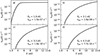Fig. 1. Probability of fragmentation and the resulting photo-dissociation rate as a function of the internal energy. See also Eq. (11). Total photo-dissociation rates were obtained by integrating along the energy axis. Panels a–d correspond to the activation energies for H and H2 loss from C60H and C60H2, as indicated in Table 2.

3.4. Photo-ionisation

The ionisation energy for C₆₀ is ∼7.65 eV (Pogulay et al. 2004):

$$\begin{array}{cc}\hfill {\mathrm{C}}_{60}{\mathrm{H}}_i+\varphi & \stackrel{k_{\mathrm{ion}}}{\to }{\mathrm{C}}_{60}{\mathrm{H}}_i^{+},\hfill \end{array}$$(15)

$$\begin{array}{cc}\hfill {\mathrm{C}}_{60}{\mathrm{H}}_i^{+}+e& \stackrel{k_{\mathrm{rec}}}{\to }{\mathrm{C}}_{60}{\mathrm{H}}_i+\varphi .\hfill \end{array}$$(16)

Pogulay et al. (2004) determined the ionisation energies for C₆₀H₁₈ and C₆₀H₃₆, at values of 7.3 eV and 7.01 eV, respectively.

We computed a photo-ionisation rate estimate by integrating the product of the ionisation cross section σ_ion and the radiation field N(E) in number of photons per second per unit area over the range of ionising photon energies:

$$\begin{array}{c}\hfill k_{\mathrm{ion}}={\displaystyle {\int }_{\mathrm{IP}}^{13.6}{\sigma }_{\mathrm{ion}}(E)N(E)\mathrm{d}E.}\end{array}$$(17)

The photo-ionisation cross section of C₆₀ has been the subject of several laboratory studies (Yasumatsu et al. 1996; Ponzi et al. 2020). An extensive study of the photo-ionisation dynamics of C₆₀ is presented in Hrodmarsson et al. (2020). As the Draine field does not vary strongly with energy for most of the considered range (up to a factor of two for energies between 7 and 12 eV), we took the ionisation cross section out of the integral and approximated it with an estimated average value. By combining the photo-absorption cross section from Berkowitz (1999) and the quantum ionisation yield presented by Yasumatsu et al. (1996), we estimated the average photo-ionisation cross section of C₆₀ to be of the order of 1.5 × 10⁻¹⁶ cm². This led to an estimated ionisation rate of

$$\begin{array}{c}\hfill k_{\mathrm{ion}}\approx 1.5\times {10}^{-16}\times {\displaystyle {\int }_{7.65}^{13.6}N(E)\mathrm{d}E\approx 1.8\times {10}^{-8}{\text{s}}^{-1}.}\end{array}$$(18)

3.5. Electron recombination

Recombination reactions can be either radiative or dissociative. To understand whether it is important to include the dissociative recombination reactions, we need to determine the branching ratio between dissociative and non-dissociative recombination. Such an analysis was carried out for carbon chain cations by Bettens & Herbst (1995), and for PAH cations by Le Page et al. (2001). Both found that the dissociative route becomes unimportant for the cations containing more than about 30 carbon atoms. This leads us to consider whether it would be justified to neglect dissociative recombination for large fullerene cations such as C₆₀H⁺ as well. An important difference between the analyses on carbon chains and PAHs is that the C−H bond energies considered in those cases were of the order of 4–5 eV. Due to its small activation energy, ∼2 eV (see also Table 2), C₆₀H should be dissociated in practically every absorption of a hard UV photon. The lower binding energy makes the dissociative route more likely, such that it may indeed be non-negligible for fullerenes, especially those in odd hydrogenation states. For C₆₀H₂ and other even numbered fulleranes that is more uncertain because their activation energy is higher (see also Table 2 and Omont 2016). For simplicity, we assumed that we could neglect the dissociative recombination reactions. This may lead us to overestimate the degree of hydrogenation, as we discuss further in Sect. 4.

The fullerene cations can return to the neutral state through electron capture and subsequent radiative relaxation:

$$\begin{array}{cc}\hfill {\mathrm{C}}_{60}{\mathrm{H}}_i^{+}+e& \stackrel{k_{\mathrm{rec}}}{\to }{\mathrm{C}}_{60}{\mathrm{H}}_i+\varphi .\hfill \end{array}$$(19)

No measurements have been made of the recombination rate for ${\text{C}}_{\text{60}}^{\text{+}}$. There are various commonly used strategies for estimating it (see also Montillaud et al. 2013).

Bakes & Tielens (1995) based their recombination rate for ${\text{C}}_{\text{60}}^{\text{+}}$ on the work by Draine & Sutin (1987) on the charge states of grains, and estimated a recombination cross section of 1.1 × 10⁻¹³ cm². This resulted in rates of an order of magnitude higher than the measured recombination rate for naphthalene, and an overestimation using this method would be consistent with the expectation of Draine & Sutin (1987) that grain surface recombination is faster than radiative recombination in the gas phase.

Le Page et al. (2001) estimated recombination rates for PAHs by taking the experimental values for benzene and naphtalene, following Salama et al. (1996). As also expressed by Ruiterkamp et al. (2005), the rate for naphtalene of 3 × 10⁻⁷ cm³ s⁻¹ was measured at 300 K (Abouelaziz et al. 1993), and can be extrapolated to any temperature as follows:

$$\begin{array}{c}\hfill k_{\mathrm{rec}}=3\times {10}^{-7}(\frac{300\mathrm{K}}{T}{)}^{\frac{1}{2}}s(e)({\text{cm}}^3{\text{s}}^{-1}),\end{array}$$(20)

where s(e) is the electron sticking coefficient, which depends mainly on the electron affinity (see the description by Allamandola et al. 1989). The sticking coefficient approaches unity when electron auto-detachment from the excited molecule can be neglected with respect to radiative relaxation. This is certainly the case for the large electron affinity of 2.67 eV, and thus we assumed s(e) = 1 for C₆₀. Thus, assuming a diffuse cloud temperature of 100 K, we obtain the following rate:

$$\begin{array}{c}\hfill k_{\mathrm{rec}}=3\times {10}^{-7}(\frac{300\text{K}}{100\text{K}}{)}^{\frac{1}{2}}\approx 1.7\times {10}^{-7}{\text{cm}}^3{\text{s}}^{-1}.\end{array}$$(21)

3.6. Radiative electron attachment

The attachment of an electron onto neutral fullerenes leads to the formation of fullerene anions:

$$\begin{array}{c}\hfill {\mathrm{C}}_{60}{\mathrm{H}}_i+e\stackrel{k_{\mathrm{rec}}}{\to }{\mathrm{C}}_{60}{\mathrm{H}}_i^{-}+\varphi .\end{array}$$(22)

We followed Ruiterkamp et al. (2005), Omont (1986), and Allamandola et al. (1989) in assuming that the electron attachment rate can be described by the Langevin collision model. The rate coefficient was computed as follows:

$$\begin{array}{c}\hfill k=2\pi \sqrt{\frac{e^2\alpha }{\mu }},\end{array}$$(23)

where α is now polarisability of neutral C₆₀, which has been determined at α = 76.5 ų = 7.65 × 10⁻²³ cm³ (Antoine et al. 1999). With the mass of the electron being negligible compared to that of C₆₀, we set the reduced mass as follows:

$$\begin{array}{c}\hfill \mu =\frac{m_e{m}_{C60}}{m_e+m_{C60}}\approx m_e=9.109\times {10}^{-28}\text{g}.\end{array}$$(24)

The elementary charge in cgs units is e = 4.80326 × 10⁻¹⁰ statC, where the statcoulomb can be written in the base units of cm^3/2 g^1/2 s⁻¹. Filling in the numbers, we find

$$\begin{array}{cc}\hfill k_e& =2\pi \times 4.8\times {10}^{-10}\text{statC}\sqrt{\frac{7.65\times {10}^{-23}{\text{cm}}^3}{9.109\times {10}^{-28}\text{g}}}\hfill \end{array}$$(25)

$$\begin{array}{cc}& \approx 8.8\times {10}^{-8}{\text{cm}}^3{\text{s}}^{-1}.\hfill \end{array}$$(26)

The work by Viggiano et al. (2010) suggests higher recombination rates of close to 10⁻⁶ cm³ s⁻¹. In this case, we would underestimate the fraction of C₆₀ in the anionic state.

3.7. Photo-detachment

We assumed that the main mechanism for neutralising ${\text{C}}_{\text{60}}^{\text{−}}$ is the photo-detachment of an electron:

$$\begin{array}{c}\hfill {\mathrm{C}}_{60}{\mathrm{H}}_i^{-}+hv\to {\mathrm{C}}_{60}{\mathrm{H}}_i+e.\end{array}$$(27)

We computed a rate estimation for electron photo-detachment by integrating the product of a photo-detachment cross section with the interstellar radiation field over energies above the electron affinity of neutral C₆₀. From Fig. 4 from Dolmatov & Manson (2022) we estimated a photo-detachment cross section of ${\text{C}}_{\text{60}}^{\text{−}}$ of the order of less than 2 Mbarn = 2 × 10⁻¹⁸ cm², which is consistent with Fig. 4 from Prabhudesai et al. (2005). This leads to a photo-detachment rate of k_ph = 1.4 × 10⁻⁹ cm³ s⁻¹.

3.8. Sources of uncertainty in reaction rates

As summarised in Table 1, the reaction rate estimations outlined above are all based on simplifying approximations. We lack an experimental reference for most of the rate coefficients, and it is not straightforward to quantify an expected range of deviation between and true reaction rates. Because our principle aim is to obtain a qualitative understanding of the hydrogenation depending on cloud structure, the computed estimates will suffice. To have an idea of how our approximations will affect the model outcomes, we point out several sources of uncertainty and expected consequences.

The main source of uncertainty in the hydrogenation balance model is the rate coefficient estimation for photo-dissociation rates, for several reasons. First, Tielens (2005) note that the effective temperature approximation overestimates the photo-dissociation rate with respect to Rice–Ramsperger–Kassel–Marcus (RRKM) theory at low internal energies (≲7 eV), possibly by orders of magnitude. Making use of this approximation may therefore lead us to underestimate the degree of hydrogenation by as much. Second, the total photo-dissociation rates we computed show a steep dependence on the binding energy: the difference between binding energies of E₀ = 3.1 eV and E₀ = 3.3 eV results in an order of magnitude difference in rate coefficients. Uncertainties in the experimental values of binding energies are therefore expected to produce significant errors in the reaction rates. Lastly, as discussed in Sect. 3.3, there is no experimental value for the binding energy per H atom of ${\text{C}}_{\text{60}}{\text{H}}_2^{\text{+}}$. So far, we have assumed it to equal the measured value for the binding energy of the H atom in C₆₀H⁺ (3.1 eV). This is almost certainly not the case, however, considering that for the neutral C₆₀H_i there is a difference between the even and odd hydrogenation states that results in a three-order-of-magnitude difference between dissociation rates. To understand the impact of this on the model outcomes, we produce and alternative abundance distribution using a dissociation rate of k_pd, +, e = 10⁻³ × k_pd, +, o.

In the present reaction network we have omitted the hydrogenation of C₆₀ through interaction with the trihydrogen cation: ${\mathrm{C}}_{60}+{\mathrm{H}}_3^{+}\to {\mathrm{C}}_{60}{\mathrm{H}}^{+}+{\mathrm{H}}_2$. However, ${\text{H}}_3^{\text{+}}$ is generally known to be a very effective proton donor and has been shown to be ubiquitously present in the ISM (McCall et al. 1998; Oka 2006). This simplification should therefore lead us to underestimate the relative abundance of C₆₀H⁺ in regions where bare, neutral C₆₀ is abundant in the gas phase.

For the charge balance we considered only photo-detachment, photo-ionisation, radiative attachment, and radiative recombination reactions. We thereby neglected dissociative recombination, associative detachment and charge transfer reactions. However, Petrie & Bohme (2000) expect the main loss channel for the C₆₀ anion to be mutual neutralisation and associative detachment with radicals such as atomic hydrogen. By not including these mechanisms we are thus likely to overestimate the ratio ${\text{C}}_{\text{60}}^{\text{−}}$:C₆₀.

4. Model description and outcomes

We set up a steady-state model for the hydrogenation of C₆₀ by adapting the work by Vuong & Foing (2000) on the hydrogenation balance of PAHs. We began by studying the cases for neutral and ionised C₆₀ separately, neglecting the photo-ionisation of C₆₀ H_i and effect of electron attachment onto C₆₀ ${\text{H}}_{\text{i}}^{\text{+}}$ on the abundance of neutral hydrogenated C₆₀. We then moved on to model the charge balance between C₆₀ in the neutral, anionic and cationic forms, before combining the hydrogenation and charge states into a single model.

Because we expect H-loss reactions to dominate strongly over H₂ loss, we neglected the loss of H₂ through photo-dissociation or dissociative attachment reactions. As explained in Sect. 3.5, we also assumed all recombination is radiative and non-dissociative. The H-loss reactions for all neutral hydrogenation states were modelled with two rates: the rate of H loss from C₆₀H was assumed for all hydrogenation states with an odd number of H atoms i, and the rate of H loss from C₆₀ H₂ was assumed for all even-numbered hydrogenation states.

4.1. C₆₀ hydrogenation balance

With this simplified model, we predicted the abundances in different hydrogenation states of C₆₀ by considering the hydrogenation of C₆₀H_i − 1 and the photo-dissociation of C₆₀H_i − 1, where 1 ≤ i ≤ n. We assumed the addition rate to be independent of i, and the dissociation rate only to depend on whether i is even or odd. As such, the model includes the following reactions:

$$\begin{array}{cc}& {\mathrm{C}}_{60}{\mathrm{H}}_{i-1}+\mathrm{H}\stackrel{k_{\mathrm{add}}}{\to }{\mathrm{C}}_{60}{\mathrm{H}}_i,\hfill \end{array}$$(28)

$$\begin{array}{cc}& {\mathrm{C}}_{60}{\mathrm{H}}_{2j}+h\nu \stackrel{k_{\mathrm{pd},\mathrm{o}}}{\to }{\mathrm{C}}_{60}{\mathrm{H}}_{2j-1}+\mathrm{H},\hfill \end{array}$$(29)

$$\begin{array}{cc}& {\mathrm{C}}_{60}{\mathrm{H}}_{2j+1}+h\nu \stackrel{k_{\mathrm{pd},\mathrm{e}}}{\to }{\mathrm{C}}_{60}{\mathrm{H}}_{2j}+\mathrm{H}.\hfill \end{array}$$(30)

Based on these equations we set up a system of steady-state equations and solved it to obtain a distribution among hydrogenation states. The derivation is presented in Appendix A. To get a qualitative sense of the model predictions, we substituted k_add = 2.3 × 10⁻¹⁰ cm⁻³s⁻¹, k_pd, o = 10⁻⁷ s⁻¹, and k_pd, e = 10⁻⁹ s⁻¹. The resulting distribution is shown in Fig. 2, where we can see that the model predicts much higher abundances for the even-numbered hydrogenation states than for the odd ones. In particular, it predicts an abundance for C₆₀H₂ of up to about half of that for fully de-hydrogenated C₆₀, depending on the environmental conditions.

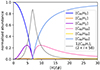Fig. 2. Distribution of abundances among hydrogenation states of C60 plotted against the hydrogen-density (cm−3)-to-flux ratio, according to the simplified model described in Sect. 4.1. Note that the model predicts significantly higher abundances for the even hydrogenation states than for the odd ones.

Because we neglected to include dissociative recombination reactions, the model for ${\text{C}}_{\text{60}}^{\text{+}}$ consists of the same set of reactions with different rates. The distribution thus looks roughly the same as for the neutral case but shifted a bit with respect to the x-axis, as can be seen in the abundance prediction according to the full hydrogenation-charge-balance model.

4.2. C₆₀ charge balance

We modelled the charge balance between bare C₆₀ cages in the anionic, neutral, and cationic states. This excludes the case of doubly ionised C₆₀, which, with an ionisation energy of about 11.3 eV Pogulay et al. (2004), might also be present in the diffuse medium. Assuming a steady state, we balanced the following detachment, attachment, ionisation, and recombination reactions:

$$\begin{array}{cc}& {\mathrm{C}}_{60}^{-}+h\nu \stackrel{k_{\det }}{\to }{\mathrm{C}}_{60}+e,\hfill \end{array}$$(31)

$$\begin{array}{cc}& {\mathrm{C}}_{60}+e\stackrel{k_{\mathrm{att}}}{\to }{\mathrm{C}}_{60}^{-}+h\nu ,\hfill \end{array}$$(32)

$$\begin{array}{cc}& {\mathrm{C}}_{60}+h\nu \stackrel{k_{\mathrm{ion}}}{\to }{\mathrm{C}}_{60}^{+}+e,\hfill \end{array}$$(33)

$$\begin{array}{cc}& {\mathrm{C}}_{60}^{+}+e\stackrel{k_{\mathrm{rec}}}{\to }{\mathrm{C}}_{60}+h\nu .\hfill \end{array}$$(34)

Setting up a system of steady-state equations, solving numerically in python, and inputting the rates as determined in the previous sections leads to the distribution shown in Fig. 3.

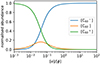Fig. 3. Predicted distribution of C60 molecules among the anionic, neutral, and cationic charge states as a function of electron density (cm−3) over radiation field strength in terms of the Draine field.

4.3. Combined model for hydrogenation and charge states

The abundances for neutral and ionised fulleranes influence each other through ionisation and recombination reactions. To combine the ionised and neutral cases, we modelled the following reactions:

$$\begin{array}{cc}& {\mathrm{C}}_{60}{\mathrm{H}}_{i-1}^{(+)}+\mathrm{H}\stackrel{k_{\mathrm{add}}}{\to }{\mathrm{C}}_{60}{\mathrm{H}}_i^{(+)},\hfill \end{array}$$(35)

$$\begin{array}{cc}& {\mathrm{C}}_{60}{\mathrm{H}}_{2j}^{(+)}+h\nu \stackrel{k_{\mathrm{pd},\mathrm{o}}}{\to }{\mathrm{C}}_{60}{\mathrm{H}}_{2j-1}^{(+)}+\mathrm{H},\hfill \end{array}$$(36)

$$\begin{array}{cc}& {\mathrm{C}}_{60}{\mathrm{H}}_{2j+1}^{(+)}+h\nu \stackrel{k_{\mathrm{pd},\mathrm{e}}}{\to }{\mathrm{C}}_{60}{\mathrm{H}}_{2j}^{(+)}+\mathrm{H},\hfill \end{array}$$(37)

$$\begin{array}{cc}& {\mathrm{C}}_{60}{\mathrm{H}}_i+h\nu \stackrel{k_{\mathrm{ion}}}{\to }{\mathrm{C}}_{60}{\mathrm{H}}_i^{+},\hfill \end{array}$$(38)

$$\begin{array}{cc}& {\mathrm{C}}_{60}{\mathrm{H}}_i^{+}+e\stackrel{k_{\mathrm{rec}}}{\to }{\mathrm{C}}_{60}{\mathrm{H}}_i.\hfill \end{array}$$(39)

Using the above reactions, we set up a system of 122 steady state equations, one for each hydrogenation and charge state combination. We then solved this system of equations numerically using python, normalising to the total abundance. This computation results in the abundance distribution shown in Fig. 4.

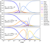Fig. 4. Model-predicted hydrogenation and charge states for fullerene C60 as a function of the hydrogen-to-flux ratio, given two different values for the photo-dissociation rate of the even-numbered cationic fulleranes, and two different values for the electron to hydrogen density ratio. Solid lines correspond to singly ionised states and dashed lines to neutral states. The solid and dashed grey lines indicate the respective sums of ion and neutral abundances that are not plotted individually (${\mathrm{\Sigma }}_{i=3}^{57}[{\mathrm{C}}_{60}{\mathrm{H}}_i^{(+)}]$). The difference between the top and centre panels demonstrates the effect of a 103 times larger photo-dissociation rate (kpd) for even compared to odd H cover. Comparison of the centre and bottom panels illustrates the effect of [e]/[H] on the hydrogenation and charge state distribution.

5. Discussion

The distribution of neutral C₆₀ among hydrogenation states as presented in Fig. 2 shows that the balance can shift from bare to fully hydrogenated within a relatively narrow range of hydrogen and flux densities. As a consequence of the much higher photo-dissociation rate for odd-numbered hydrogenation states, our model predicts significantly higher abundances of C₆₀ in the even than in the odd hydrogenation states.

The predicted distribution of C₆₀ among three charge states shown in Fig. 3 indicates a sharp transition from ionised to neutral to anionic forms at an electron-to-flux ratio of about 0.01 to 0.1. For an electron density of around 7.5 × 10⁻³ times the hydrogen density (Bakes & Tielens 1995), taking the radiation field to be the un-reddened Draine field and assuming an atomic hydrogen density between 10 and 100 cm⁻¹, it follows that diffuse interstellar clouds provide the environmental conditions in which the balance shifts from the cation to neutral to the anion. The model predicts that the relative abundance of the neutral never exceeds about 15%, and the ratio C₆₀:${\text{C}}_{\text{60}}^{\text{+}}$ is maximised at about 0.4.

The steady-state model-predicted distribution of C₆₀ among charge and hydrogenation states presented in Fig. 4 shows a clear sensitivity to the uncertain reaction rates. The differences in photo-dissociation rates between the top and centre panels and in terms of electron density between the centre and bottom panels result in very different abundance distributions. Nonetheless, by investigating our model outcomes for a selection of parameter values, we can make some general predictions for the charge and hydrogenation states of C₆₀ in diffuse interstellar environments.

We recognise the pattern of hydrogenation from Fig. 2 when looking at the dashed lines in the centre panel of Fig. 4. This indicates that the hydrogenation balance of the neutral and the cation influence each other. This is also clear when comparing the top and centre panels of Fig. 4, where the shift from bare to hydrogenated occurs in approximately the same environmental conditions for both the neutral and ionised species, even though a rate coefficient has only been changed for the cation.

To compare the combined distribution with the charge distribution in Fig. 3, we first note that ${\text{C}}_{\text{60}}^{\text{−}}$ was not included in the combined model. The dashed lines in Fig. 4 could therefore more accurately be interpreted as the sum of abundances in the neutral and anionic states. Although the inclusion of the anionic hydrogenation states in this model will be left for future work, we can already state that this will lead to much lower neutral abundance predictions, especially for the more fully hydrogenated states. Comparing the top and centre panels in Fig. 4, we see that the overall charge distribution predicted by the model is not affected by hydrogenation. This is as expected because we assumed the ionisation and recombination rates to be the same for all hydrogenation states. The centre and bottom panels of Fig. 4 are model outcomes computed with about an order of magnitude difference in the electron-to-hydrogen ratios. This amounts to about a ten times smaller recombination rate for the bottom panel with respect to the centre panel, and has the consequence that the charge balance is shifted to higher hydrogen densities. For the lower electron-to-hydrogen ratio (Fig. 4, bottom panel), nearly all the C₆₀ molecules in partially hydrogenated states are therefore ionised.

5.1. Implications for diffuse cloud environments

To see how the abundance prediction as a function of the atomic hydrogen abundance to UV flux ratio translates to a prediction for particular diffuse cloud environmental conditions, we modelled the UV flux inside a cloud as a function of reddening, E(B − V). This was achieved by multiplying the Draine interstellar radiation field by the average extinction curve from Cardelli et al. (1989). In order to understand the effect of reddening on the chemistry, we carried out the computations for the photo-reaction rates using extincted radiation fields for a range of reddening values. The resulting reaction rates are shown in Fig. 5. We used this figure to determine a range of reasonable hydrogen-to-flux ratios, [H]/[ϕ], when studying the abundance distribution shown in Fig. 4: the atomic hydrogen density for diffuse clouds is typically about 1–100 cm⁻¹. Figure 5 tells us that the effects of reddening can increase this ratio by typically less than an order of magnitude for E_B − V ∼ 1. Depending on the exact environmental parameters, we can thus expect that 1 ≲ [H]/[ϕ]≲10³ for diffuse interstellar clouds. With this in mind, and looking back at Fig. 4, we note that the dominant combinations of hydrogenation and charge states are${\text{C}}_{\text{60}}^{\text{+}}$, C₆₀H⁺, C₆₀, and C₆₀H₆₀. However, regarding the fully hydrogenated species, we note that the geometrical strain introduced by hydrogenation beyond 36 H atoms is expected from calculations to lead to the formation of isomers with one or more of the C−H bonds pointing inwards (creating more isomer possibilities and thereby resulting in weaker bands; Dunlap et al. 1991) and can cause the fragmentation and thus complete destruction of the C₆₀ molecule (Zhang et al. 2020).

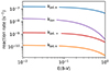Fig. 5. Variation in rates for radiation-driven reactions with reddening, E(B − V), within the cloud environment.

Some molecules are easier to observe than others due to factors such as symmetry, oscillator strength, or simply the interstellar abundance. Even with simple models, such as those presented here, we can use observations of these species to learn something about related compounds as well. Our model predictions suggest that C₆₀H⁺ may be abundant in the diffuse medium. This is in line with the suggestion by Kroto & Jura (1992) that C₆₀H⁺ should be the most commonly occurring fullerene analogue in the ISM. C₆₀H⁺ has only one isomer configuration due to the symmetry of the C₆₀ cage, leading to relatively strong bands. The infrared spectrum of C₆₀H⁺ was recently measured by Palotás et al. (2020), who find that the symmetry breaking as a consequence of protonation results in a much richer IR spectrum as compared to bare C₆₀. Not much has been reported about the electronic spectral features of C₆₀H⁺; therefore, we are not (yet) in a position to compare laboratory spectral rest wavelengths to interstellar observations of DIBs. A confirmation of the interstellar presence of C₆₀H⁺ would provide invaluable insights into the hydrogenation networks of fullerenes. A detection with an inferred abundance with respect to bare ${\text{C}}_{\text{60}}^{\text{+}}$, or even an upper limit, would allow us to place constraints on the rest of the hydrogenation network as well.

5.2. Suggestions for future work

Based on the insight gained from the theoretical study we have carried out, we can make several suggestions for future theoretical, experimental, and observational research. In this section, we briefly summarise our suggestions along each of the three lines of inquiry.

There are a number of adaptations that can be made in order to improve our theoretical model. First, we estimated the photo-dissociation rates using an effective temperature approximation following Tielens (2005). These rates can be made more accurate through the application of RRKM theory, or an adapted version such as that from Le Page et al. (2001). Second, by studying the charge balance separately we have shown that it is important to include ${\text{C}}_{\text{60}}^{\text{−}}$ in the full hydrogenation and charge balance model. This will eventually rely on experimental studies on the hydrogenation of ${\text{C}}_{\text{60}}^{\text{−}}$. Similarly, it should be investigated how inclusion of the double cation C${}_{60}^{2+}$ would affect our model-predicted abundance distributions, considering that the ionisation energy of ${\text{C}}_{\text{60}}^{\text{+}}$ (∼11.3 eV) is lower than that of hydrogen. Lastly, the model can be improved by expanding the reaction network to include charge transfer and associative detachment reactions to increase the accuracy of the charge balance estimation, and by including proton transfer reactions with the trihydrogen cation. We find conditions where neutral C₆₀ could be present for high values of e/H, as displayed in the centre panel of Fig. 4. To search for C₆₀, one should look for lines of sight with those special conditions to detect C₆₀ absorption lines at 398 nm and possibly around 622 nm, as measured in the gas phase by Sassara et al. (2001). It would be useful to apply our model to make a prediction of what we can expect to observe towards specific environments along well-constrained sightlines. In particular, the BD+63° sightline provides an interesting reference when searching for hydrogenated fullerenes because it crosses more UV-shielded environments (Ehrenfreund et al. 1997; Tuairisg et al. 2000).

Experimental measurements of the relevant reaction rates would likely significantly improve the accuracy of our model predictions. And importantly, in order to work towards the identification of DIBs, there would be a great use for laboratory spectroscopic measurements of hydrogenated fullerenes and C₆₀H⁺ in particular. Even matrix isolation spectra can be helpful, as illustrated by the example of the ${\text{C}}_{\text{60}}^{\text{+}}$ DIBs.

Based on our findings, we suggest the following observational research:

• Surveys of the C₆₀H⁺ IR transition bands (Palotás et al. 2020) towards different sightlines with a variation of environmental parameters and different strengths of the ${\text{C}}_{\text{60}}^{\text{+}}$ DIBs.

• The continued study of (anti-)correlations between the ${\text{C}}_{\text{60}}^{\text{+}}$ DIBs and other DIBs as a function of environmental parameters, such as UV radiation, in order to catalogue which DIBs could in theory originate from C₆₀-related compounds, such as hydrogenated ${\text{C}}_{\text{60}}^{\text{+}}$ (although a correlation or anti-correlation would certainly not imply such a chemical relation directly).

• DIBs have been relatively under-sampled in the near-infrared region of the spectrum given the difficulties presented by telluric contamination. Near-infrared DIB surveys have the potential to provide important new ways to test our understanding of the interstellar chemistry of large carbonaceous molecules because ${\text{C}}_{\text{60}}^{\text{−}}$ is expected to have transitions in this spectral region. For this purpose, we continue to carry out observations at the Isaac Newton Telescope, which may bring promising new insights in future work.

Acknowledgments

We dedicate this article to Professor Harold Linnartz, and thank him for his support throughout the Master Research project. DA thanks the anonymous referee for providing valuable comments to the manuscript. DA gratefully acknowledges support from LUNEX EuroMoonMars EuroSpaceHub for the Master research project, and INT observing campaign. DA received further funding from the Leiden University Trustee Funds. This work has made use of NASA’s Astrophysics Data System Bibliographic Services; Scipy, a free and open-source Python library used for scientific computing and technical computing (Virtanen et al. 2021); Astropy (http://www.astropy.org) a community-developed core Python package and an ecosystem of tools and resources for astronomy (Astropy Collaboration 2013, 2018, 2022), and the Astropy affiliated Interstellar Dust Extinction package.

References

Appendix A: Derivation of the hydrogenation balance

We can then write the steady state equations as follows:

$$\begin{array}{cc}\hfill \frac{d[C_{60}{H}_i]}{\mathit{dt}}=0& ={\displaystyle \sum }\text{gains}-\sum \text{losses},\hfill \end{array}$$(A.1)

$$\begin{array}{cc}& =k_{\mathrm{add}}[C_{60}{H}_{i-1}][H]-k_{\mathrm{pd}}[C_{60}{H}_i][{\varphi }_{\nu }],\hfill \end{array}$$(A.2)

where we distinguish between the even and odd dissociation rates k_pd, e and k_pd, o for even and odd i, respectively. It follows that

$$\begin{array}{c}\hfill \frac{[C_{60}{H}_i][{\varphi }_{\nu }]}{[C_{60}{H}_{i-1}][H]}=\frac{k_{\mathrm{add}}}{k_{\mathrm{pd}}}.\end{array}$$(A.3)

For brief notation, we defined a hydrogenation rate balance, x_even/odd, between successive hydrogenation states as follows:

$$\begin{array}{c}\hfill x_{\mathrm{e}/\mathrm{o}}=\frac{[H]}{[{\varphi }_{\nu }]}\times \frac{k_{\mathrm{add}}}{k_{\mathrm{pd},\mathrm{e}/\mathrm{o}}}=\frac{[C_{60}{H}_i]}{[C_{60}{H}_{i-1}]},\end{array}$$(A.4)

This allows us to write the abundance of C₆₀ in hydrogenation state i with respect to fully de-hydrogenated C₆₀ as

$$\begin{array}{c}\hfill \frac{[C_{60}{H}_i]}{[C_{60}]}=\underset{x_{\mathrm{even}/\mathrm{odd}}}{\underbrace{\frac{[C_{60}{H}_i]}{[C_{60}{H}_{i-1}]}}}\times \underset{x_{\mathrm{odd}/\mathrm{even}}}{\underbrace{\frac{[C_{60}{H}_{i-1}]}{[C_{60}{H}_{i-2}]}}}\times ···\times \underset{x_{\mathrm{odd}}}{\underbrace{\frac{[C_{60}{H}_1]}{[C_{60}{H}_0]}}}.\end{array}$$(A.5)

Now, explicitly distinguishing between the even and odd hydrogenation states by introducing the index j and recognising the recurring terms in the above equation, we can write the abundances in terms of the rate balance:

$$\begin{array}{cc}\hfill \frac{[C_{60}{H}_{2j}]}{[C_{60}]}& =x_{\mathrm{even}}^j{x}_{\mathrm{odd}}^j,\hfill \end{array}$$(A.6)

$$\begin{array}{cc}\hfill \frac{[C_{60}{H}_{2j+1}]}{[C_{60}]}& =x_{\mathrm{even}}^j{x}_{\mathrm{odd}}^{j+1}.\hfill \end{array}$$(A.7)

Normalising to the total abundance,

$$\begin{array}{c}\hfill {\displaystyle \sum _{i=0}^n[C_{60}{H}_i]=1,}\end{array}$$(A.8)

we obtain

$$\begin{array}{cc}\hfill 1& ={\displaystyle \sum _{j=0}^{\frac{n}{2}}[C_{60}{H}_0]\frac{[C_{60}{H}_i]}{[C_{60}{H}_0]}+\sum _{j=0}^{\frac{n}{2}-1}[C_{60}{H}_0]\frac{[C_{60}{H}_i]}{[C_{60}{H}_0]},}\hfill \end{array}$$(A.9)

$$\begin{array}{cc}& ={\displaystyle \sum _{j=0}^{\frac{n}{2}}[C_{60}{H}_0]{(x_{\mathrm{e}}{x}_{\mathrm{o}})}^j+\sum _{j=0}^{\frac{n}{2}-1}[C_{60}{H}_0]x_{\mathrm{e}}^j{x}_{\mathrm{o}}^{j+1},}\hfill \end{array}$$(A.10)

$$\begin{array}{cc}& \Rightarrow [C_{60}{H}_0]=[{\displaystyle \sum _{j=0}^{\frac{n}{2}}{(x_{\mathrm{e}}{x}_{\mathrm{o}})}^j+\sum _{j=0}^{\frac{n}{2}-1}{x}_{\mathrm{e}}^j{x}_{\mathrm{o}}^{j+1}{]}^{-1}.}\hfill \end{array}$$(A.11)

At this point we recognise the partial sum of the geometric series in the denominator:

$$\begin{array}{cc}\hfill {\displaystyle \sum _{i=0}^n}{(x_H)}^i& =1+x+x^2+···x^n,\hfill \end{array}$$(A.12)

$$\begin{array}{cc}& =\frac{1}{x-1}([x+x^2+···+x^{n+1}]\hfill \end{array}$$(A.13)

$$\begin{array}{cc}& -[1+x+x^2+···+x^n]),\hfill \end{array}$$(A.14)

$$\begin{array}{cc}& =\frac{1}{x-1}(x^{n+1}-1),\hfill \end{array}$$(A.15)

$$\begin{array}{cc}& =\frac{x^{n+1}-1}{x-1}.\hfill \end{array}$$(A.16)

Inserting this and rearranging, we find

$$\begin{array}{c}\hfill [C_{60}{H}_0]=\frac{x_{\mathrm{e}}{x}_{\mathrm{o}}-1}{{(x_{\mathrm{e}}{x}_{\mathrm{o}})}^{\frac{n}{2}+1}(1+x_{\mathrm{e}}^{-1})-x_{\mathrm{o}}-1}.\end{array}$$(A.17)

This leads to the following expressions for the abundance distribution among hydrogenation states:

$$\begin{array}{cc}\hfill [C_{60}{H}_{2j}]& =x_{\mathrm{e}}^j{x}_{\mathrm{o}}^j[C_{60}{H}_0],\hfill \end{array}$$(A.18)

$$\begin{array}{cc}& =x_{\mathrm{e}}^j{x}_{\mathrm{o}}^j\frac{x_{\mathrm{e}}{x}_{\mathrm{o}}-1}{{(x_{\mathrm{e}}{x}_{\mathrm{o}})}^{\frac{n}{2}+1}(1+x_e^{-1})-x_{\mathrm{o}}-1},\hfill \end{array}$$(A.19)

$$\begin{array}{cc}& =x_{\mathrm{e}}^j{x}_{\mathrm{o}}^{j+1}[C_{60}{H}_0],\hfill \end{array}$$(A.20)

$$\begin{array}{cc}& =x_{\mathrm{o}}[C_{60}{H}_{2j}].\hfill \end{array}$$(A.21)

All Tables

All Figures

	Fig. 1. Probability of fragmentation and the resulting photo-dissociation rate as a function of the internal energy. See also Eq. (11). Total photo-dissociation rates were obtained by integrating along the energy axis. Panels a–d correspond to the activation energies for H and H2 loss from C60H and C60H2, as indicated in Table 2.
In the text

	Fig. 2. Distribution of abundances among hydrogenation states of C60 plotted against the hydrogen-density (cm−3)-to-flux ratio, according to the simplified model described in Sect. 4.1. Note that the model predicts significantly higher abundances for the even hydrogenation states than for the odd ones.
In the text

	Fig. 3. Predicted distribution of C60 molecules among the anionic, neutral, and cationic charge states as a function of electron density (cm−3) over radiation field strength in terms of the Draine field.
In the text

Fig. 4. Model-predicted hydrogenation and charge states for fullerene C60 as a function of the hydrogen-to-flux ratio, given two different values for the photo-dissociation rate of the even-numbered cationic fulleranes, and two different values for the electron to hydrogen density ratio. Solid lines correspond to singly ionised states and dashed lines to neutral states. The solid and dashed grey lines indicate the respective sums of ion and neutral abundances that are not plotted individually (${\mathrm{\Sigma }}_{i=3}^{57}[{\mathrm{C}}_{60}{\mathrm{H}}_i^{(+)}]$). The difference between the top and centre panels demonstrates the effect of a 103 times larger photo-dissociation rate (kpd) for even compared to odd H cover. Comparison of the centre and bottom panels illustrates the effect of [e]/[H] on the hydrogenation and charge state distribution.

In the text

	Fig. 5. Variation in rates for radiation-driven reactions with reddening, E(B − V), within the cloud environment.
In the text

References

- Abouelaziz, H., Gomet, J. C., Pasquerault, D., Rowe, B. R., & Mitchell, J. B. A. 1993, J. Chem. Phys., 99, 237 [NASA ADS] [CrossRef] [Google Scholar]
- Allamandola, L. J., Tielens, A. G. G. M., & Barker, J. R. 1989, ApJS, 71, 733 [Google Scholar]
- Andrews, H., Candian, A., & Tielens, A. G. G. M. 2016, A&A, 595, A23 [NASA ADS] [CrossRef] [EDP Sciences] [Google Scholar]
- Antoine, R., Dugourd, P., Rayane, D., et al. 1999, J. Chem. Phys., 110, 9771 [NASA ADS] [CrossRef] [Google Scholar]
- Astropy Collaboration (Robitaille, T. P., et al.) 2013, A&A, 558, A33 [NASA ADS] [CrossRef] [EDP Sciences] [Google Scholar]
- Astropy Collaboration (Price-Whelan, A. M., et al.) 2018, AJ, 156, 123 [Google Scholar]
- Astropy Collaboration (Price-Whelan, A. M., et al.) 2022, ApJ, 935, 167 [NASA ADS] [CrossRef] [Google Scholar]
- Bakes, E., & Tielens, A. G. G. M. 1995, Astrophys. Space Sci. Libr., 202, 315 [NASA ADS] [CrossRef] [Google Scholar]
- Berkowitz, J. 1999, J. Chem. Phys., 111, 1446 [NASA ADS] [CrossRef] [Google Scholar]
- Bettens, R. P. A., & Herbst, E. 1995, Int. J. Mass Spectr. Ion Proc., 149, 321 [CrossRef] [Google Scholar]
- Bettinger, H. F., Rabuck, A. D., Scuseria, G. E., et al. 2002, Chem. Phys. Lett., 360, 509 [NASA ADS] [CrossRef] [Google Scholar]
- Briggs, J. B., & Miller, G. P. 2010, Fulleranes, 2, 105 [NASA ADS] [CrossRef] [Google Scholar]
- Brühwiler, P. A., Andersson, S., Dippel, M., et al. 1993, Chem. Phys. Lett., 214, 45 [CrossRef] [Google Scholar]
- Cami, J., Bernard-Salas, J., Peeters, E., & Malek, S. E. 2010, Science, 329, 1180 [NASA ADS] [CrossRef] [Google Scholar]
- Campbell, E. K., Holz, M., Gerlich, D., & Maier, J. P. 2015, Nature, 523, 322 [NASA ADS] [CrossRef] [Google Scholar]
- Cardelli, J. A., Clayton, G. C., & Mathis, J. S. 1989, ApJ, 345, 245 [Google Scholar]
- Castellanos, P., Candian, A., Zhen, J., Linnartz, H., & Tielens, A. G. G. M. 2018, A&A, 616, A166 [NASA ADS] [CrossRef] [EDP Sciences] [Google Scholar]
- Cataldo, F., & Iglesias-Groth, S. 2009, MNRAS, 400, 291 [NASA ADS] [CrossRef] [Google Scholar]
- Cataldo, F., & Iglesias-Groth, S. 2010, Fulleranes: The Hydrogenated Fullerenes, Carbon Materials: Chemistry and Physics, (Dordrecht: Springer), 2 [CrossRef] [Google Scholar]
- Cataldo, F., García-Hernández, D. A., Manchado, A., & Iglesias-Groth, S. 2014, IAU Symp., 297, 294 [NASA ADS] [Google Scholar]
- Cox, N. L. J., & Cami, J. 2014, IAU Symp., 297, 412 [NASA ADS] [Google Scholar]
- Cox, N. L. J., Cami, J., Farhang, A., et al. 2017, A&A, 606, A76 [NASA ADS] [CrossRef] [EDP Sciences] [Google Scholar]
- Demarais, N. J., Yang, Z., Snow, T. P., & Bierbaum, V. M. 2014, ApJ, 784, 25 [NASA ADS] [CrossRef] [Google Scholar]
- Dolmatov, V. K., & Manson, S. T. 2022, Atoms, 10, 99 [CrossRef] [Google Scholar]
- Draine, B. T., & Sutin, B. 1987, ApJ, 320, 803 [NASA ADS] [CrossRef] [Google Scholar]
- Dunlap, B. I., Brenner, D. W., Mintmire, J. W., Mowrey, R. C., & White, C. T. 1991, J. Phys. Chem., 95, 5763 [CrossRef] [Google Scholar]
- Ehrenfreund, P., Cami, J., Dartois, E., & Foing, B. H. 1997, A&A, 318, L28 [NASA ADS] [Google Scholar]
- Foing, B. H., & Ehrenfreund, P. 1994, Nature, 369, 296 [NASA ADS] [CrossRef] [Google Scholar]
- Foing, B. H., & Ehrenfreund, P. 1997, A&A, 317, L59 [NASA ADS] [Google Scholar]
- Heger, M. L. 1922, Lick Obs. Bull., 10, 146 [NASA ADS] [Google Scholar]
- Henderson, C. C., McMichael Rohlfing, C., & Cahill, P. A. 1993, Chem. Phys. Lett., 213, 383 [NASA ADS] [CrossRef] [Google Scholar]
- Herbig, G. H. 1995, ARA&A, 33, 19 [Google Scholar]
- Herbst, E., & Dunbar, R. C. 1991, MNRAS, 253, 341 [CrossRef] [Google Scholar]
- Hrodmarsson, H. R., Garcia, G. A., Linnartz, H., & Nahon, L. 2020, Phys. Chem. Chem. Phys., 22, 13880 [Google Scholar]
- Jolibois, F., Klotz, A., Gadéa, F. X., & Joblin, C. 2005, A&A, 444, 629 [NASA ADS] [CrossRef] [EDP Sciences] [Google Scholar]
- Kaiser, A., Leidlmair, C., Bartl, P., et al. 2013, J. Chem. Phys., 138, 074311 [NASA ADS] [CrossRef] [Google Scholar]
- Kroto, H. W., & Jura, M. 1992, A&A, 263, 275 [Google Scholar]
- Kroto, H. W., Heath, J. R., O’Brien, S. C., Curl, R. F., & Smalley, R. E. 1985, Nature, 318, 162 [NASA ADS] [CrossRef] [Google Scholar]
- Lange, K., Dominik, C., & Tielens, A. G. G. M. 2021, A&A, 653, A21 [NASA ADS] [CrossRef] [EDP Sciences] [Google Scholar]
- Le Page, V., Snow, T. P., & Bierbaum, V. M. 2001, ApJS, 132, 233 [NASA ADS] [CrossRef] [Google Scholar]
- Leidlmair, C., Bartl, P., Schöbel, H., et al. 2011, ApJ, 738, L4 [NASA ADS] [CrossRef] [Google Scholar]
- Linnartz, H., Cami, J., Cordiner, M., et al. 2020, J. Mol. Spectr., 367, 111243 [NASA ADS] [CrossRef] [Google Scholar]
- McCall, B. J., Geballe, T. R., Hinkle, K. H., & Oka, T. 1998, Science, 279, 1910 [CrossRef] [Google Scholar]
- Merrill, P. W. 1934, PASP, 46, 206 [NASA ADS] [CrossRef] [Google Scholar]
- Miller, T. M., & Bederson, B. 1978, in Advances in Atomic and Molecular Physics, eds. D. R. Bates, & B. Bederson (Academic Press), 13, 1 [NASA ADS] [CrossRef] [Google Scholar]
- Montillaud, J., Joblin, C., & Toublanc, D. 2013, A&A, 552, A15 [NASA ADS] [CrossRef] [EDP Sciences] [Google Scholar]
- Oka, T. 2006, Proc. Nat. Academy Sci., 103, 12235 [NASA ADS] [CrossRef] [Google Scholar]
- Omont, A. 1986, A&A, 164, 159 [NASA ADS] [Google Scholar]
- Omont, A. 2016, A&A, 590, A52 [NASA ADS] [CrossRef] [EDP Sciences] [Google Scholar]
- Palotás, J., Martens, J., Berden, G., & Oomens, J. 2020, Nat. Astron., 4, 240 [Google Scholar]
- Petrie, S., & Bohme, D. K. 2000, ApJ, 540, 869 [NASA ADS] [CrossRef] [Google Scholar]
- Petrie, S., Becker, H., Baranov, V. I., & Bohme, D. K. 1995, Int. J. Mass Spectr. Ion Proc., 145, 79 [NASA ADS] [CrossRef] [Google Scholar]
- Pogulay, A. V., Abzalimov, R. R., Nasibullaev, S. K., et al. 2004, Int. J. Mass Spectr., 233, 165 [NASA ADS] [CrossRef] [Google Scholar]
- Ponzi, A., Manson, S. T., & Decleva, P. 2020, J. Phys. Chem. A, 124, 108 [NASA ADS] [CrossRef] [Google Scholar]
- Prabhudesai, V. S., Nandi, D., & Krishnakumar, E. 2005, Eur. Phys. J. D, 35, 261 [NASA ADS] [CrossRef] [Google Scholar]
- Ruiterkamp, R., Cox, N. L. J., Spaans, M., et al. 2005, A&A, 432, 515 [NASA ADS] [CrossRef] [EDP Sciences] [Google Scholar]
- Salama, F., Bakes, E. L. O., Allamandola, L. J., & Tielens, A. G. G. M. 1996, ApJ, 458, 621 [NASA ADS] [CrossRef] [Google Scholar]
- Sassara, A., Zerza, G., Chergui, M., & Leach, S. 2001, ApJS, 135, 263 [NASA ADS] [CrossRef] [Google Scholar]
- Schröder, D., Bohme, D. K., Weiske, T., & Schwarz, H. 1992, Int. J. Mass Spectr. Ion Proc., 116, R13 [CrossRef] [Google Scholar]
- Snow, T. P., & McCall, B. J. 2006, AJ, 50 [Google Scholar]
- Spieler, S., Kuhn, M., Postler, J., et al. 2017, ApJ, 846, 168 [NASA ADS] [CrossRef] [Google Scholar]
- Tielens, A. G. G. M. 2005, The Physics and Chemistry of the Interstellar Medium (Cambridge: Cambridge University Press) [Google Scholar]
- Tielens, A. G. G. M., & Snow, T. P. 1995, Astrophys. Space Sci. Libr., 202 [CrossRef] [Google Scholar]
- Tuairisg, S. Ó., Cami, J., Foing, B. H., Sonnentrucker, P., & Ehrenfreund, P. 2000, A&AS, 142, 225 [NASA ADS] [CrossRef] [EDP Sciences] [Google Scholar]
- Vehviläinen, T. T., Ganchenkova, M. G., Oikkonen, L. E., & Nieminen, R. M. 2011, Phys. Rev. B, 84, 085447 [CrossRef] [Google Scholar]
- Viggiano, A. A., Friedman, J. F., Shuman, N. S., et al. 2010, J. Chem. Phys., 132, 194307 [NASA ADS] [CrossRef] [Google Scholar]
- Virtanen, P., Gommers, R., Burovski, E., et al. 2021, https://doi.org/10.5281/zenodo.4718897 [Google Scholar]
- Vuong, M. H., & Foing, B. H. 2000, A&A, 363, L5 [NASA ADS] [Google Scholar]
- Walker, G. A. H., Bohlender, D. A., Maier, J. P., & Campbell, E. K. 2015, ApJ, 812, L8 [NASA ADS] [CrossRef] [Google Scholar]
- Walker, G. A. H., Campbell, E. K., Maier, J. P., Bohlender, D., & Malo, L. 2016, ApJ, 831, 130 [CrossRef] [Google Scholar]
- Yasumatsu, H., Kondow, T., Kitagawa, H., Tabayashi, K., & Shobatake, K. 1996, J. Chem. Phys., 104, 899 [NASA ADS] [CrossRef] [Google Scholar]
- Zhang, Y., Sadjadi, S., & Hsia, C.-H. 2020, Astrophys. Space Sci., 365, 67 [NASA ADS] [CrossRef] [Google Scholar]