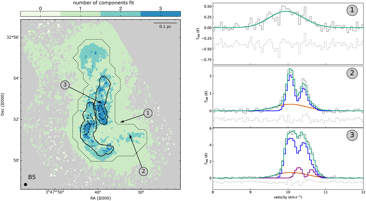
Number of components detected towards different parts of B5, as decided by the Bayesian approach described in Sect. 3.1 (left). These components are then subdivided into 5 separate components according to their velocities (see Sect. 3.2). The black-solid and black-dashed contours show the two filaments and the three condensations in B5, respectively (contours adapted from Schmiedeke et al. 2021). The black-dotted contour shows the boundary of the coherent core in Pineda et al. (2010). The beam size and scale-bar are shown in the bottom-left and the top-right corners, respectively. Examples of NH₃ (1,1) spectra from regions with one-, two-, and three-component fits (right, with the positions of the spectra indicated in the left panel). Only a small range in velocity is shown here to clearly highlight the individual components, which are illustrated in blue, red, and purple. In each panel, the fitted model is shown in green, while the residuals are shown in grey. Note: there are multiple, closely-spaced hyperfines in the velocity range shown here. The strongest two of these hyperfines can be seen in the narrow component (blue and purple in panels 2 and 3). However, these hyperfines are blended together in the broad component (green in panel 1, red in panels 2 and 3), and therefore the hyperfine structure is not visible.