| Issue |
A&A
Volume 681, January 2024
|
|
|---|---|---|
| Article Number | L14 | |
| Number of page(s) | 7 | |
| Section | Letters to the Editor | |
| DOI | https://doi.org/10.1051/0004-6361/202348367 | |
| Published online | 15 January 2024 | |
Letter to the Editor
FlopPITy: Enabling self-consistent exoplanet atmospheric retrievals with machine learning
1
Kapteyn Astronomical Institute, University of Groningen, Groningen, The Netherlands
e-mail: This email address is being protected from spambots. You need JavaScript enabled to view it.
2
Netherlands Space Research Institute (SRON), Leiden, The Netherlands
3
Centre for Exoplanet Science, University of Edinburgh, Edinburgh, UK
4
School of GeoSciences, University of Edinburgh, Edinburgh, UK
Received:
23
October
2023
Accepted:
20
December
2023
Abstract
Context. Interpreting the observations of exoplanet atmospheres to constrain physical and chemical properties is typically done using Bayesian retrieval techniques. Since these methods require many model computations, a compromise must be made between the model’s complexity and its run time. Achieving this compromise leads to a simplification of many physical and chemical processes (e.g. parameterised temperature structure).
Aims. Here, we implement and test sequential neural posterior estimation (SNPE), a machine learning inference algorithm for atmospheric retrievals for exoplanets. The goal is to speed up retrievals so they can be run with more computationally expensive atmospheric models, such as those computing the temperature structure using radiative transfer.
Methods. We generated 100 synthetic observations using ARtful Modeling Code for exoplanet Science (ARCiS), which is an atmospheric modelling code with the flexibility to compute models across varying degrees of complexity and to perform retrievals on them to test the faithfulness of the SNPE posteriors. The faithfulness quantifies whether the posteriors contain the ground truth as often as we expect. We also generated a synthetic observation of a cool brown dwarf using the self-consistent capabilities of ARCiS and ran a retrieval with self-consistent models to showcase the possibilities opened up by SNPE.
Results. We find that SNPE provides faithful posteriors and is therefore a reliable tool for exoplanet atmospheric retrievals. We are able to run a self-consistent retrieval of a synthetic brown dwarf spectrum using only 50 000 forward model evaluations. We find that SNPE can speed up retrievals between ∼2× and ≥10× depending on the computational load of the forward model, the dimensionality of the observation, and its signal-to-noise ratio (S/N). We have made the code publicly available for the community on Github.
Key words: methods: statistical / planets and satellites: atmospheres / brown dwarfs
© The Authors 2024
 Open Access article, published by EDP Sciences, under the terms of the Creative Commons Attribution License (https://creativecommons.org/licenses/by/4.0), which permits unrestricted use, distribution, and reproduction in any medium, provided the original work is properly cited.
This article is published in open access under the Subscribe to Open model. This email address is being protected from spambots. You need JavaScript enabled to view it. to support open access publication.
1. Introduction
Interpreting exoplanet and brown dwarf observations to estimate the physical and chemical properties of their atmospheres is typically done using Bayesian inference to find the joint posterior probability distribution of model parameters. This posterior is traditionally found using sequential sampling-based inference methods, most commonly Markov chain Monte Carlo (MCMC) or different nested sampling algorithms, particularly Multinest (Feroz et al. 2009). This is a computationally expensive process, often requiring hundreds of thousands to millions of forward model evaluations to converge.
The high computational expense essentially limits the use of complex atmospheric models in retrievals, making it necessary to reach a compromise between model complexity and compute time. The model complexity arises from including more realistic physics, for instance, computing self-consistently the temperature structure and cloud formation or including disequilibrium chemistry. Models that take more than a second to run already push a single retrieval to between a day and two weeks depending on the number of model evaluations needed. In addition, higher spectral resolution or larger wavelength coverage with new instruments increase the size of the data set and are often coupled with higher sensitivities, for instance, by JWST (Gardner et al. 2006). Together, these cause inference methods to require more model evaluations to converge, easily reaching 107 evaluations based on retrievals in Barrado et al. (2023).
In order to speed up retrievals and enable analyses of more detailed observations with more complex models, machine learning retrieval methods have started to be developed (e.g. Waldmann 2016; Zingales & Waldmann 2018; Márquez-Neila et al. 2018; Cobb et al. 2019; Nixon & Madhusudhan 2020; Yip et al. 2021, 2022; Ardévol Martínez et al. 2022; Vasist et al. 2023).
These previous studies have shown that machine learning can provide constraints compatible with those obtained with Multinest. In particular, Ardévol Martínez et al. (2022) demonstrated that the parameter constraints obtained with machine learning retrievals are extremely reliable. However, in this previous approach, the posterior was approximated by a multivariate Gaussian. With good enough data, it might be a reasonable assumption, however, this is not yet the case for exoplanet atmospheres; so the reliability has come at the expense of inaccurate posterior shapes. To correct this, Vasist et al. (2023) developed a normalizing flow based retrieval framework that removed the assumption of Gaussianity, endowing it with the capability to reproduce the shape of nested sampling posteriors.
The vast majority of previous approaches have been amortised estimators. This means that after training, they are suitable to perform inference on observations occupying any region of parameter space. To accomplish this a large enough training set covering the full parameter space in sufficient resolution is required. As we already explained in detail in Ardévol Martínez et al. (2022, see Sect. 3.4) the need for a large training set leads to an inflexibility with regard to the atmospheric model that has been adopted.
To counteract this shortcoming, Yip et al. (2022) developed a machine learning retrieval framework based on variational inference and normalising flows that was able to reproduce accurately nested sampling posteriors using < 10% of the forward models while retaining the same flexibility. However, this approach requires the atmospheric model to be differentiable and so we would need to either use Diff-τ (the differentiable model developed by Yip et al. 2022) or develop new differentiable models, limiting its usability.
Here we present FlopPITy (normalising FLOw exoPlanet Parameter Inference ToolkYt), a machine learning retrieval framework based on neural spline flows (Durkan et al. 2019) and sequential neural posterior estimation (SNPE, Greenberg et al. 2019). This approach retains the flexibility of sampling-based methods while requiring only a fraction of the forward model evaluations. Additionally, it works with any atmospheric modelling code without the need to rewrite it or adapt it.
In this Letter, we first describe briefly the machine learning approach we use in Sect. 2. In Sect. 3 we apply FlopPITy to synthetic observations to test and showcase its performance. Section 4 discusses the implications of these results and the advantages and shortcomings of our method. Finally, in Sect. 5, we present our conclusions.
2. (Sequential) neural posterior estimation
Normalising FLOw exoPlanet Parameter Inference ToolkYt (FlopPITy)1 is a new tool for exoplanet atmospheric retrievals that uses sequential neural posterior estimation. In particular, we use Automatic Posterior Transformation (APT or SNPE-C, Greenberg et al. 2019) as implemented in the python package SBI (Tejero-Cantero et al. 2020). SNPE-C belongs to a larger group of likelihood-free inference methods, which are useful when the likelihood function is intractable. In our case, the likelihood can be calculated, so the advantage of SNPE is the speed-up that the use of machine learning provides. SNPE-C approximates the posterior distribution, p(θ|x) with the distribution qF(x, ϕ)(θ|x), where q is a density family2 and F is a neural network with weights, ϕ. In this work we use normalizing flows (Papamakarios et al. 2021) for our posterior estimator, qF. We refer to Appendix A in Vasist et al. (2023) for a brief overview on normalizing flows. More specifically, we use neural spline flows (Durkan et al. 2019), for which a more palatable explanation can be found in Green & Gair (2021).
Amortised estimators such as those presented in Ardévol Martínez et al. (2022) and Vasist et al. (2023) are incredibly convenient since once they are trained, inferences can be carried out almost instantly for any observation. However, they are relatively inflexible. Observational details and data processing choices (e.g. wavelength range used, spectral resolution, noise properties, etc.) are fixed during training, which means that for real world usage the estimator needs to be retrained with the observational properties of each observation. The main source of inflexibility comes from the need to pre-compute large training sets covering the whole prior parameter space, limiting the use cases for the trained estimator. This is because simple changes like adding extra chemical species to the models imply computing a whole new training set. Additionally, this large upfront computational cost, although lower than would be required for Multinest, can still be unfeasible for more complex models.
Here we present a non-amortised approach that is as flexible as traditional sampling-based retrievals. Like the latter, it requires computing new forward models for every retrieval. However it needs only a fraction of them compared to nested sampling, resulting in a significant speed-up.
We use SNPE-C with multi-round training as described in Greenberg et al. (2019). The way it works is as follows: initially, N parameter vectors, θi, are drawn from the prior, and corresponding forward models, xi, are computed. These are used to train the estimator and obtain a first approximation to the posterior. From this posterior, we draw another N amount samples and compute the corresponding forward models, which we use to improve the training and obtain an improved estimate for the posterior distribution. Figure 1 illustrates how the method works. After the first round of training the estimator is no longer amortised but is only suitable for the specific observation we are analysing. This process is repeated for a set number of rounds. Unfortunately, because after the first round we are not sampling from the prior p(θ) but, instead, a so-called proposal distribution  ; furthermore, the resulting distribution is no longer the true posterior p(θ|x), but, rather, a so-called proposal posterior:
 (1)
(1)
where
 (2)
(2)
SNPE-C automatically transforms between estimates of the true posterior and the proposal posterior, making it easy to sample the estimated true posterior. The interested reader can consult Greenberg et al. (2019) for details of how this can be accomplished.
Since SNPE-C uses qF(x, ϕ)(θ) to approximate the posterior, from Eq. (1) we can approximate the proposal posterior as  . We train the network by minimizing the loss function:
 (3)
(3)
This yields qF(x, ϕ)(θ)→p(x|θ) and  as N → ∞ (Papamakarios & Murray 2016). The proposal prior is then defined as
  , where x0 is the data.
This sequential approach is not without caveats, as it can provide overconfident posteriors (Hermans et al. 2022). However we have not found that to be the case and this is discussed in more detail in Sect. 3.
The observational error is accounted for by adding noise to the simulated spectra. Training is done on noisy samples  with ε ∈ 𝒩(0, σ0), where xi are the simulated spectra, 𝒩(μ, σ) is the normal distribution, and σ0 the observed noise. Because the network has already learnt the noise, at the time of inference only x0 is passed.
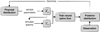 |
Fig. 1. Schematic representation of the iterative training of a neural spline flow. In the very first iteration, the proposal distribution is the prior. |
3. Mock retrievals
We tested FlopPITy on two scenarios. First, we ran retrievals using a simple and fast atmospheric model to test its reliability. Subsequently, we ran a retrieval using a complex, computationally expensive atmospheric model to showcase the science cases that this methods enables.
3.1. Bulk retrievals
We performed retrievals on a hundred synthetic NIRSpec PRISM spectra to test the faithfulness of our method. For the purpose of illustration, we used a relatively simple (computationally fast) atmospheric model to minimise the computational load.
The synthetic observations were generated using ARCiS (Min et al. 2020) with an isothermal temperature structure T(p) = T0, free H2O and CO2 abundances, and the radius, RP, and log g of the planet. The parameter ranges from which the synthetic spectra were sampled are the same as the prior ranges used for the retrievals, and are shown in Table A.1. The spectroscopic channels and observational noise are taken from the FIREFLy reduction in Rustamkulov et al. (2023).
To perform the retrievals, we trained FlopPITy in 20 rounds using 1000 simulations in each round. Such a high number of rounds is not necessary but this allows us to check if training for more rounds than necessary leads to overconfidence. We also performed Multinest retrievals on the simulated observations to have a baseline to compare against.
We then wanted to check that the posteriors produced by our method are correctly estimated and are not too broad or too narrow. We do this by calculating the expected coverage probability following Hermans et al. (2022) and Vasist et al. (2023). The coverage probability is the probability of a certain confidence region containing the ground truth. If the posteriors were correctly estimated, a region of the posterior with a fraction (1 − α)% of the probability would contain the ground truth (1 − α)% of the time. Figure 2 shows the coverage probability for the posteriors produced at each round. Its interpretation is simple: if the coverage probability is below the diagonal, the posteriors are overconfident (too narrow), whereas if the coverage probability is above, posteriors are underconfident (too wide).
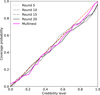 |
Fig. 2. Coverage probability of SNPE posteriors at different training rounds compared to Multinest. The red dashed line denotes the 1:1 line. All the lines are close to the diagonal, indicating that both the Multinest and SNPE posteriors are faithful. Importantly, the latter remain faithful at every round. |
Although the curves in Fig. 2 are a bit noisy due to computational feasibility limiting the number of mock retrievals, they follow the diagonal closely at each training round, showing a performance on par with that of Multinest. Crucially, Fig. 2 shows that the posteriors do not become increasingly overconfident with subsequent training iterations, but are reliable at each step. Figure 2 seems to indicate that at high credibility levels, FlopPITy is slightly overconfident when compared to Multinest. A larger number of mock retrievals would have to be run to feasibly ascertain whether it is a real effect or just an artifact. If real, it would indicate that the probability in the wings of the posteriors is underestimated and therefore care should be taken not to overinterpret them.
3.2. Self-consistent retrieval
To showcase the real power of FlopPITy, we performed a retrieval with a self-consistent setup on a simulated observation of a brown dwarf. We generate the synthetic observation using the self-consistent capabilities of ARCiS. We assume a 1D (cloud-free) atmosphere in radiative-convective equilibrium (with an effective temperature, Teff) as well as thermochemical equilibrium computed from the carbon to oxygen ratio, C/O, and metallicity, Z, and we included chemical disequilibrium due to vertical mixing (Kawashima & Min 2021). The vertical mixing is parameterised by the eddy diffusion coefficient Kzz. We used the best-fitting parameters for the cool Y dwarf WISE 1828+2650 (De Furio et al. 2023). We generated a spectrum with R = 1000 in the wavelength range 5 − 18 μm. We assumed an error on the flux of 10−5 Jy, corresponding to a signal-to-noise ratio (S/N) between ∼0 and ∼40, depending on the wavelength. This result is representative of what can be achieved in most of the MIRI MRS wavelength range when binned down to R = 1000 (Barrado et al. 2023). The model parameters and their priors are shown in Table A.2. We do not show a comparison to a Multinest retrieval as it is not computationally feasible.
We trained FlopPITy in ten rounds, using 5000 forward models in each round. We used a larger simulation budget than in the previous case because the mapping from atmospheric parameters to spectra is more complex. In the simple model case, changes in parameters directly affect the spectrum, for instance, a higher molecular abundance increases the amplitude of the features in the spectrum. For the self-consistent model this is no longer the case. For example, the molecular abundances (which influence the amplitude of the spectral features) depend on the internal temperature, the carbon-to-oxygen ratio, the metallicity, and the vertical diffusion.
To account for possible biases due to the noise realization of an individual observation, we generated five different noisy observations from the simulated spectrum and aggregated the posteriors retrieved. The corresponding corner plot can bee seen in Fig. 3, with all parameters being faithfully recovered.
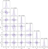 |
Fig. 3. Posteriors for five noise realizations of a synthetic WISE 1828+2650 spectrum. The input parameters of the synthetic spectrum are denoted by the black lines and are: Teff = 325 K, RP = 1.83RJ, log g = 3.6, log Kzz = 7, C/O = 0.55, and log Z = 0. To keep the figure readable, we show only the 2σ contours. The quantiles shown in the titles correspond to one of the noisy realisations. |
Figure 3 shows that for the S/N considered, we can get errors of ∼1% on crucial evolutionary properties, such as Teff, R and log g. This is only the case when the model perfectly reproduces the observation. For real data, this will never be the case as there would always be physical and chemical processes that have not been taken into account by the model. In this case it is unknown what level of precision and bias one should expect and even the extent to which the retrievals remain reliable. There might also be differences in performance between FlopPITy and Multinest, which would make one or the other a better option in specific cases. These questions will be explored in future work.
4. Discussion
We show that FlopPITy, an implementation of SNPE-C with neural spline flows, is a reliable method for exoplanet and brown dwarf atmospheric retrievals and it allows us to perform retrievals using forward models that are too slow for traditional sampling-based retrievals. In particular, the retrieval performed on the simulated brown dwarf spectrum (Sect. 3.2) used 50 000 simulations in total, taking ∼18 h to complete on a 2020 M1 MacBook Pro. This time was split in ∼15 h for the computation of the simulations and ∼3 h for training. Based on the retrievals ran in Barrado et al. (2023), we can estimate that the same retrieval with Multinest would require between 500 000 and 1 500 000 model evaluations to converge. Since each forward model requires ∼3 s to run, such a retrieval would take at least ∼20 days to converge.
As a comparison, the simple retrievals took ∼3 h each in a cluster with 48 AMD Opteron 6348 processors, out of which ∼1 h 25 min were used for training. Their Multinest counterparts typically needed between 20 000 and 60 000 forward models to converge, taking between 3 and 8 hours. Higher S/N observations typically require more forward models for Multinest to converge. The lower (to no) computational advantage of FlopPITy over Multinest in this case is due to two factors. First, having a simpler dataset (with lower spectral resolution by a factor of ∼6) results in Multinest requiring fewer model evaluations to converge. Second, using a faster forward model (∼0.5 s versus ∼3 s) means that the training ends up representing a significant fraction of the time needed for the FlopPITy retrieval.
This means that for simpler datasets and faster forward models, our method does not provide a substantial speed up compared to Multinest, and for very simple datasets (e.g. HST WFC3 spectra), Multinest might even be preferred. Conversely, FlopPITy enables analyses of complex datasets with computationally costly atmospheric models that would otherwise not be feasible with sampling-based retrieval methods.
Additionally, Multinest has the disadvantage that models need to be computed sequentially, so it can not be parallelised3. Yet, SNPE does not have this limitation and the computation of the forward models can be spread over multiple CPUs, further speeding up retrievals.
The sequential approach presented here is not universally preferable to amortised approaches such as the one in Vasist et al. (2023). In particular, if the goal is to perform retrievals on a large number of spectra using the same atmospheric model (as will undoubtedly be the case for future missions such as ARIEL, Tinetti et al. 2018), an amortised approach will be computationally more efficient. However for the exploration of a single dataset, our sequential approach is more appropriate as the extra flexibility allows to more easily try and compare different atmospheric models with different assumptions.
The main drawback of FlopPITy is the need to choose how many rounds to train for and how many training examples to use per round. Fortunately, as we have shown in Sect. 3.1, the posteriors do not become overconfident by training for too many rounds. Nevertheless, training for more rounds than necessary represents an unnecessary computational expense that we would like to avoid. A way to gauge the convergence of the retrieval is to compare the posteriors at consecutive rounds, and train for a few more rounds if there is still significant variation. The 1σ, 2σ, and 3σ envelopes of the retrieved spectra can also be used to ensure that the posterior is not overdispersed. Regarding the amount of training examples, ideally, it would be possible to choose as many as computationally affordable. Due to the stochastic nature of the random sampling of parameter vectors in the prior and proposal distributions, using too few examples will result in an uneven coverage of the parameter space, which could have a negative effect on the results.
Finally, it is still unclear how FlopPITy or nested sampling respond to adversarial examples. These are observations with features that are not well reproduced by the model, which we coined ‘uncomfortable retrievals’ in Ardévol Martínez et al. (2022). There we showed that machine learning was more reliable than Multinest when the observations were not well reproduced by the underlying atmospheric model. However, this came at the expense of very broad posteriors, so the information gain over the prior was limited (which is still preferred to biased posteriors). In future works, we will explore if FlopPITy can remain reliable in this scenario, while being more informative than the machine learning retrievals in Ardévol Martínez et al. (2022), or if it instead behaves more similarly to Multinest.
5. Conclusions
In this Letter we present FlopPITy, a new machine learning retrieval tool that uses normalizing flows and multi-round training and we demonstrate that it works reliably.
In contrast with previous machine learning retrieval methods, this method retains the flexibility of sampling-based methods and is applicable to any atmospheric model, requiring only a fraction of the forward models needed by the latter, with the exact fraction depending on the specific observation and model used. When performing individual retrievals, the sequential approach presented here requires fewer models to train on than amortised approaches, as the computational effort is focused in the relevant regions of parameter space. However, once it is trained, amortised estimators are able to perform retrievals almost instantly and are therefore better suited for the analysis of large datasets with the same forward model.
Our method enables retrievals of high quality observations, such as those provided by JWST, with computationally costly forward models, for instance, self-consistent temperature structure or cloud formation. This reduces the need to simplify atmospheric models to speed them up for retrievals, although of course it does not eliminate it completely, as there are still tens of thousands of forward models that need to be computed in a reasonable time frame. Additionally, unlike with sampling-based retrievals, the computation of these models can be parallelised over multiple CPUs, further speeding up a retrieval. This work highlights the avenues that machine learning is opening for characterizing exoplanets and expands the suite of existing machine learning retrieval methods and their use cases.
FlopPITy can be accessed at https://github.com/franciscoardevolmartinez/FlopPITy
A density family is a group of probability distributions described by the same parameters. Examples of density families include the: Gaussian distribution, Gaussian mixture with N components, or binomial distribution.
A small level of parallelization can be achieved by simultaneously drawing N points at each nested sampling iteration, with 1/N being an estimate of the sampling efficiency.
Acknowledgments
We would like to thank the Center for Information Technology of the University of Groningen for their support and for providing access to the Peregrine high performance computing cluster. This research has made use of NASA’s Astrophysics Data System. This project has received funding from the European Union’s Horizon 2020 research and innovation programme under the Marie Sklodowska-Curie grant agreement No. 860470. We would like to thank Malavika Vasist for fruitful discussions. We are thankful to Beatriz Campos Estrada, whose comments helped improve the manuscript. We are also grateful to Daniel Talaván Vega, who came up with the name FlopPITy over half a decade ago. P.I.P. acknowledges funding from the STFC consolidator grant #ST/V000594/1.
References
- Ardévol Martínez, F., Min, M., Kamp, I., & Palmer, P. I. 2022, A&A, 662, A108 [NASA ADS] [CrossRef] [EDP Sciences] [Google Scholar]
- Barrado, D., Mollière, P., Patapis, P., et al. 2023, Nature, 624, 263 [NASA ADS] [CrossRef] [Google Scholar]
- Cobb, A. D., Himes, M. D., Soboczenski, F., et al. 2019, AJ, 158, 33 [NASA ADS] [CrossRef] [Google Scholar]
- De Furio, M., Lew, B., Beichman, C., et al. 2023, ApJ, 948, 92 [Google Scholar]
- Durkan, C., Bekasov, A., Murray, I., Papamakarios, G., et al. 2019, in Advances in Neural Information Processing Systems, eds. H. Wallach, H. Larochelle, A. Beygelzimer, et al. (Curran Associates, Inc.), 32 [Google Scholar]
- Feroz, F., Hobson, M. P., & Bridges, M. 2009, MNRAS, 398, 1601 [NASA ADS] [CrossRef] [Google Scholar]
- Gardner, J. P., Mather, J. C., Clampin, M., et al. 2006, Space Sci. Rev., 123, 485 [Google Scholar]
- Green, S. R., & Gair, J. 2021, Mach. Learn. Sci. Technol., 2, 03LT01 [CrossRef] [Google Scholar]
- Greenberg, D., Nonnenmacher, M., & Macke, J. 2019, in Proceedings of the 36th International Conference on Machine Learning, eds. K. Chaudhuri, & R. Salakhutdinov, Proc. Mach. Learn. Res., 97, 2404 [Google Scholar]
- Hermans, J., Delaunoy, A., Rozet, F., et al. 2022, Trans. Mach. Learn. Res. https://openreview.net/forum?id=LHAbHkt6Aq [Google Scholar]
- Kawashima, Y., & Min, M. 2021, A&A, 656, A90 [NASA ADS] [CrossRef] [EDP Sciences] [Google Scholar]
- Márquez-Neila, P., Fisher, C., Sznitman, R., & Heng, K. 2018, Nat. Astron., 2, 719 [CrossRef] [Google Scholar]
- Min, M., Ormel, C. W., Chubb, K., Helling, C., & Kawashima, Y. 2020, A&A, 642, A28 [NASA ADS] [CrossRef] [EDP Sciences] [Google Scholar]
- Nixon, M. C., & Madhusudhan, N. 2020, MNRAS, 496, 269 [NASA ADS] [CrossRef] [Google Scholar]
- Papamakarios, G., & Murray, I. 2016, in Proceedings of the 30th International Conference on Neural Information Processing Systems, NIPS’16 (Red Hook, NY, USA: Curran Associates Inc.), 1036 [Google Scholar]
- Papamakarios, G., Nalisnick, E., Rezende, D. J., Mohamed, S., & Lakshminarayanan, B. 2021, J. Mach. Learn. Res., 22, 1 [Google Scholar]
- Rustamkulov, Z., Sing, D. K., Mukherjee, S., et al. 2023, Nature, 614, 659 [NASA ADS] [CrossRef] [Google Scholar]
- Tejero-Cantero, A., Boelts, J., Deistler, M., et al. 2020, J. Open Source Software, 5, 2505 [NASA ADS] [CrossRef] [Google Scholar]
- Tinetti, G., Drossart, P., Eccleston, P., et al. 2018, Exp. Astron., 46, 135 [NASA ADS] [CrossRef] [Google Scholar]
- Vasist, M., Rozet, F., Absil, O., et al. 2023, A&A, 672, A147 [NASA ADS] [CrossRef] [EDP Sciences] [Google Scholar]
- Waldmann, I. P. 2016, ApJ, 820, 107 [NASA ADS] [CrossRef] [Google Scholar]
- Yip, K. H., Changeat, Q., Nikolaou, N., et al. 2021, AJ, 162, 195 [NASA ADS] [CrossRef] [Google Scholar]
- Yip, K. H., Changeat, Q., Al-Refaie, A., & Waldmann, I. 2022, ApJ, submitted [arXiv:2205.07037] [Google Scholar]
- Zingales, T., & Waldmann, I. P. 2018, AJ, 156, 268 [NASA ADS] [CrossRef] [Google Scholar]
Appendix A: Retrieval priors
The tables below contain the priors used in the retrievals shown in the text.
Bulk retrieval priors.
Self-consistent retrieval priors.
Appendix B: When inference fails
Both Multinest and FlopPITy can fail in certain situations. Here we show one example from the bulk retrievals in 3.1 where the posterior has a narrow mode around the ground truth which is completely missed by both retrieval methods, as visible in Fig. B.1.
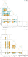 |
Fig. B.1. Example corner plots for a case with a very narrow posterior around the ground truth for retrievals run with broad (top) and tight (bottom) priors. |
In a scenario that is more representative of real world retrievals, the priors on RP and log g would be significantly narrower, as these quantities can be measured from the white light curve and radial velocity, respectively. When we redo the retrievals using such narrow priors, we see that both methods find the right mode (Fig. B.1bottom).
An essential diagnosis for any inference method is to run simulations for samples drawn from the posterior and compare them to the data. As can be seen in Fig. B.2, this would make it evident that the retrieval with broad priors is not finding the right solution.
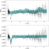 |
Fig. B.2. 1σ contours of the retrieved spectra for the case with broad (top) and tight (bottom) priors. |
This example does not correspond to a physically plausible atmosphere. Since the spectra are sampled randomly from a large parameter space, not all combinations correspond to realistic atmospheres (in this particular case, the high temperature and low gravity causes most of the atmosphere to escape). This is not an issue since we are only interested in seeing if the retrieval methods can find the parameters that gave rise to the simulation. The case presented here is simply a nice illustration of a possible failure mode for Multinest and FlopPITy.
Appendix C: Training hyperparameters
Table C.1 shows the training hyperparameters as well as the neural spline flow structure used.
Technical details of our implementation.
All Tables
All Figures
|
Fig. 1. Schematic representation of the iterative training of a neural spline flow. In the very first iteration, the proposal distribution is the prior. |
| In the text | |
|
Fig. 2. Coverage probability of SNPE posteriors at different training rounds compared to Multinest. The red dashed line denotes the 1:1 line. All the lines are close to the diagonal, indicating that both the Multinest and SNPE posteriors are faithful. Importantly, the latter remain faithful at every round. |
| In the text | |
|
Fig. 3. Posteriors for five noise realizations of a synthetic WISE 1828+2650 spectrum. The input parameters of the synthetic spectrum are denoted by the black lines and are: Teff = 325 K, RP = 1.83RJ, log g = 3.6, log Kzz = 7, C/O = 0.55, and log Z = 0. To keep the figure readable, we show only the 2σ contours. The quantiles shown in the titles correspond to one of the noisy realisations. |
| In the text | |
|
Fig. B.1. Example corner plots for a case with a very narrow posterior around the ground truth for retrievals run with broad (top) and tight (bottom) priors. |
| In the text | |
|
Fig. B.2. 1σ contours of the retrieved spectra for the case with broad (top) and tight (bottom) priors. |
| In the text | |
Current usage metrics show cumulative count of Article Views (full-text article views including HTML views, PDF and ePub downloads, according to the available data) and Abstracts Views on Vision4Press platform.
Data correspond to usage on the plateform after 2015. The current usage metrics is available 48-96 hours after online publication and is updated daily on week days.
Initial download of the metrics may take a while.