| Issue |
A&A
Volume 681, January 2024
|
|
|---|---|---|
| Article Number | A48 | |
| Number of page(s) | 11 | |
| Section | Astronomical instrumentation | |
| DOI | https://doi.org/10.1051/0004-6361/202347220 | |
| Published online | 09 January 2024 | |
Using the Gerchberg–Saxton algorithm to reconstruct nonmodulated pyramid wavefront sensor measurements
1
University of California Santa Cruz,
1156 High St,
Santa Cruz,
USA
e-mail: This email address is being protected from spambots. You need JavaScript enabled to view it.
2
Herzberg Astronomy and Astrophysics,
5071 West Saanich Road Victoria,
British Columbia
V9E 2E7,
Canada
3
Lawrence Livermore National Laboratory,
7000 East Ave.,
Livermore,
CA
94550,
USA
4
University of Arizona,
Steward Observatory,
Tucson,
AZ,
USA
5
Centre for Advanced instrumentation Lower Mount Joy,
South Rd,
Durham
DH1 3LS,
UK
6
Waka Consulting,
4 rue Joseph Bouchayer,
38100
Grenoble,
France
Received:
17
June
2023
Accepted:
25
September
2023
Abstract
Context. Adaptive optics (AO) is a technique for improving the resolution of ground-based telescopes by correcting optical aberrations due to atmospheric turbulence and the telescope itself in real time. With the rise of giant segmented-mirror telescopes (GSMT), AO is needed more than ever to reach the full potential of these future observatories. One of the main performance drivers of an AO system is the wavefront-sensing operation, consisting of measuring the shape of the optical aberrations described above.
Aims. The nonmodulated pyramid wavefront sensor (nPWFS) is a wavefront sensor with high sensitivity, allowing the limits of AO systems to be pushed. The high sensitivity comes at the expense of its dynamic range, which makes it a highly nonlinear sensor. We propose here a novel way to invert nPWFS signals by using the principle of reciprocity of light propagation and the Gerchberg-Saxton (GS) algorithm.
Methods. We tested the performance of this reconstructor in two steps: the technique was first implemented in simulations, where some of its basic properties were studied. Then, the GS reconstructor was tested on the Santa Cruz Extreme Adaptive optics Laboratory (SEAL) testbed, located at the University of California Santa Cruz.
Results. This new way to invert the nPWFS measurements allows us to drastically increase the dynamic range of the reconstruction for the nPWFS, pushing the dynamics close to a modulated PWFS. The reconstructor is an iterative algorithm with a high computational burden, which could be an issue for real-time purposes in its current implementation. However, this new reconstructor could still be helpful for various wavefront-control operations. This reconstruction technique has also been successfully tested on the Santa Cruz Extreme AO Laboratory (SEAL) bench, where it is now used as the standard way to invert nPWFS signal.
Key words: instrumentation: adaptive optics / instrumentation: high angular resolution
© The Authors 2024
 Open Access article, published by EDP Sciences, under the terms of the Creative Commons Attribution License (https://creativecommons.org/licenses/by/4.0), which permits unrestricted use, distribution, and reproduction in any medium, provided the original work is properly cited.
This article is published in open access under the Subscribe to Open model. This email address is being protected from spambots. You need JavaScript enabled to view it. to support open access publication.
1 Introduction
The pyramid wavefront sensor (PWFS; Ragazzoni 1996) is a Fourier-filtering wavefront sensor (Fauvarque 2017). These sensors are commonly used to measure aberrations in optical systems. Inspired by the Foucault knife test, the original PWFS consists of a four-sided glass pyramid located at an intermediate focal plane and a detector that captures images of the four pupils created by each beam passing through the different faces of the pyramid. This configuration efficiently converts phase into intensity, but it lacks the necessary dynamic range to accurately measure atmospheric turbulence aberrations, which can induce optical path differences on the order of several waves. To address this issue, the PWFS is often paired with a modulator that causes the electromagnetic (EM) field to circulate around the pyramid tip during the camera acquisition time. Modulation drastically improves the PWFS linearity, but it has three main drawbacks. First, the modulation leads to a strong decrease in PWFS sensitivity, especially for low-order modes. Second, modulation of the PWFS alters the nature of the signal (Vérinaud 2004; Guyon 2005), causing the response to resemble that of a slope sensor, which makes it difficult to detect phase discontinuities. This is particularly problematic for the next generation of giant segmented-mirror telescopes (GSMTs), where wavefront control will involve correcting not only for turbulence-induced aberrations, but also for those induced by the telescope itself (fragmentation, Schwartz et al. 2017; Bertrou-Cantou et al. 2022; Demers et al. 2022 and segmentation Chanan et al. 1998). Finally, adding the modulation mirror stage requires the use of more optics and leads to difficulties related to fast-steering components (stability issues, temperature constrains, speed limitations, failure risks, etc.). Therefore, extending the dynamic range of the nonmodulated PWFS (nPWFS) to remove the need for modulation could allow the use of the PWFS at its full potential while removing the requirement for moving parts, making it a less complex system. Many studies have been conducted to mitigate PWFS nonlinearities, and several options have been suggested. It was proposed to keep the matrix formalism and consider the PWFS as a linear varying-parameter system: the reconstruction matrix evolves according to the phase to be measured (Korkiakoski et al. 2008; Deo et al. 2019), but this technique usually requires some knowledge of the statistics of the measured phase (Chambouleyron et al. 2020). Gradient-descent methods have also been investigated (Frazin 2018; Hutterer et al. 2023). Finally, another approach that is more appealing today is to use a machine-learning approach to reconstruct the nPWFS signal (Landman & Haffert 2020; Nousiainen et al. 2022; Archinuk et al. 2023).
The goal of this paper is to present a novel approach to invert the nPWFS signal. This approach is based on the principle of reciprocity of light propagation and the Gerchberg-Saxton (GS) algorithm. In Sect. 2, we present the principle of the reconstruction algorithm in detail. Section 3 assesses the basic performance of the reconstructor mainly in terms of dynamic range, but also in terms of noise propagation and broadband performance. Section 4 highlights the results of an experimental implementation of this new reconstructor on the Santa Cruz Extreme Adaptive optics Laboratory (SEAL) testbed (Jensen-Clem et al. 2021). Finally, Sect. 5 describes a possible way to push the dynamic range and convergence speed of this reconstructor even further by using sensor fusion.
2 New method for inverting a nonmodulated PWFS signal
2.1 Reciprocity of the light-propagation principle
The reconstructor presented in this paper relies on one of the most basic properties of light propagation: the principle of reciprocity of the light propagation. The idea is to construct a high-fidelity numerical model of the nPWFS and use the measurements to send the light backward in the numerical nPWFS. This technique can be applied to any Fourier-filtering wavefront sensor, but we focus on the nPWFS in this study.
The numerical model of the nPWFS was built by propagating the light assuming Fraunhofer approximation from one pupil plane to the next while it passes through the pyramid mask in an intermediate focal plane. In more detail, the EM-field in the nPWFS detector plane can be written as
 (1)
(1)
where Ψp is the EM-field in the entrance pupil, m is the complex shape of the pyramid mask, ★ is the convolution product, and  denotes the Fourier-transform operator. Equation (1) allows us to simply simulate the light propagation from the entrance pupil plane to the WFS detector plane. The back-propagation of light from the detector plane to the entrance pupil plane is
 (2)
(2)
where  is the conjugate operator. This last equation can simply be understood in the nPWFS case: we write m as m = eiΔ, where Δ is a 2D real function describing the phase corresponding to the pyramid shape. Passing the pyramid in the opposite direction means that the light propagates through the inverse phase mask, that is,
  . We can then write the entrance pupil and detector EM-fields in their complex form,
 (3)
(3)
where Ap and Ad are the amplitudes, and ϕp and ϕd are the phases of the electromagnetic fields. The goal of wavefront sensing is to recover the phase ϕp in the entrance pupil. Light back-propagation cannot easily be performed from the detector measurements because we only have access to intensities in the detector plane  .The phase ϕd is therefore missing in the measurements. Hence, we propose to use an iterative algorithm called the Gerchberg-Saxton (GS) algorithm to propagate the light back and forth in the numerical model of the nPWFS.
2.2 Gerchberg-Saxton algorithm
The GS algorithm was first proposed by Gerchberg (1972) and is widely used to perform image sharpening from point spread function (PSF) images (Fienup 1982; Ragland et al. 2016). To perform this algorithm in our case, we assumed that we have access to a measurement of the entrance pupil amplitude Ap (we show an easy practical way to obtain this quantity with the nPWFS below). In the nPWFS framework, we have two complex quantities (Eq. (3)) for which the amplitudes are known and with a relation that links them (Eq. (1)). The principle of the GS algorithm is to propagate the light back and forth in the numerical model of the nPWFS, injecting the knowledge of the amplitudes of the complex quantities we are trying to retrieve at each step. We propose to go through one iteration of the GS algorithm applied to the nPWFS based on the schematic given in Fig. 1. The amplitude for the entrance pupil and the detector plane used for this example are true measurements from the SEAL testbed (highlighted with yellow dots). One iteration of the GS algorithm can be split into four parts:
- 1.
We compute the detector EM-field complex amplitude
 . For the first iteration, the complex EM-field in the detector plane is built by using
  , which corresponds to the phase in the detector plane when a flat wavefront is propagated through the nPWFS system. We therefore have a first estimate Ψd that can be back-propagated in the system (through Eq. (2)).
 - 2.
A first estimation of Ψp is then obtained.
- 3.
Because we already have access to Ap, the amplitude found through back-propagation is discarded and replaced by the measurement of Ap while keeping the estimated phase ϕp. The entrance pupil plane EM-field can then be propagated in the system (direct propagation, through Eq. (1)).
- 4.
A new estimation of Ψd is obtained. As previously done for the entrance pupil plane, we discard the amplitude and replace it by the measurement of Ad given by the detector and keep the estimated phase ϕd. We can then return to step 1 and iterate again. We call one iteration of the GS algorithm the numerical operation that consists of these four steps.
The GS algorithm is therefore an iterative algorithm, which for one iteration performs four fast Fourier transforms (FFTs). It is important to note that this reconstructor assumes coherence of the EM-field. Therefore, this algorithm does not work for the modulated PWFS. It also raises the question of the impact of measurements with larger spectral bandpasses, which we discuss in the next section. We also emphasize that this GS principle can be applied to any FFWFS, but we focus on the nPWFS here.
2.3 Phase unwrapping
The phase, ϕp, retrieved by the algorithm is wrapped, modulo 2π, as optical propagation is done. Therefore, when working with a phase with an amplitude larger than 2π peak to valley (PtV), it is necessary to add a step to the reconstruction process: a phase-unwrapping algorithm applied to the phase estimated through the GS reconstruction. A detailed analysis of this step is beyond the scope of this study, and therefore, we restrain ourselves to using a well-known simpler algorithm based on Ghiglia & Romero (1994) throughout this paper.
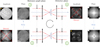 |
Fig. 1 Principle of the GS algorithm applied to nonmodulated PWFS. The yellow dots highlight the fact that these are true data obtained on the SEAL testbed. |
3 Performance of the GS algorithm reconstructor
This section gives a first overview of the basic performance of the GS algorithm. We focus on the performance of this reconstructor in terms of dynamic range, but also evaluate the number of iterations needed, the noise propagation, and the broadband impact on reconstruction. This study is not meant to be exhaustive, and parameters such as the minimum number of pixels needed on the detector with respect to the phase amplitude to be measured are not assessed, nor do we offer a detailed analysis of the impact of model errors. All the simulations simply match the SEAL testbed configuration. The main simulation parameters are the following ones: each pupil on the PWFS detector has 106 pixels across (matching the SEAL testbed configuration), which is a realistic case because the best low read-out-noise (RON) cameras can run at a few kHz with resolutions of about 250 px × 250 px. We use a Shannon sampling of 2 (4 pixels per λ/D) for the nPWFS model. For a more realistic simulation, the phase screens were first simulated and propagated with a resolution four times higher (4×106 px across) through a high-resolution model of the nPWFS with a Shannon sampling of 2 as well. The signal was then binned to produce the nPWFS image with 106 px across. We worked with a modal basis of the first 500 Zernike modes (excluding piston), which is close to the control space that can be achieved with the deformable mirrors installed on the SEAL testbed. The linear reconstructor was created in a standard fashion by building an interaction matrix and computing its pseudo-inverse. No modes were filtered during the inversion because the measurements are oversampled. This led to a good conditioning number of the interaction matrix. The simulations tools we used were sourced internally, except for the turbulent phase screens, which were created using the HCIpy library (Por et al. 2018).
3.1 Convergence speed and first comparison with a linear reconstructor
The first test we present was meant to provide an idea of the convergence speed of the GS reconstruction. It is also be a way to draw a first comparison between the linear model and our reconstructor. To do this, we studied the reconstruction of four different turbulent phase screens following a Von-Karman spectrum and corresponding to four different configurations of D/r0, where D is the telescope diameter, and r0 is the Fried parameter. To produce a fair comparison between the linear reconstructor and the GS reconstructor, which gives the phase with a much higher resolution (106 px across), these screens were projected on the 500 Zernike modes basis before propagation (no aliasing). The reconstruction error was estimated at each GS iteration (the estimated phase was systematically unwrapped) and is expressed as the ratio of the rms error in the entrance pupil plane (error = rmsrec/rmsinput).
The results are plotted in Fig. 2. The GS reconstruction accuracy increases with the number of iterations before it stabilizes. The shorter the phase, the fewer iterations are needed to reach the best reconstruction. Hence, for D/r0 = 1, only 10 iterations are required, whereas more than 1000 iterations are required for D/r0 = 32 (corresponding to a value of r0 = 25 cm for a D = 8 m telescope). This figure also shows that in any case and after a few iterations, the GS reconstructor performs better than the linear reconstructor. In the small-phase regime (in our context, this would correspond to regimes smaller than D/r0 ≈ 0.5), both perform equally well because the nPWFS would be working in its linear range. To illustrate reconstruction products, the input phase and reconstructed phases (linear and GS after 2000 iterations) for D/r0 = 32 are shown in Fig. 3. It is clear that even if the GS reconstruction still underestimates the phase (due to nPWFS saturation; this is discussed in more detail in Sect. 4.3), the shape of the retrieved phase is much more similar than the shape produced by the linear reconstructor. As a side note, the phase of the shape given by the linear reconstructor is highly underestimated, and the pattern seems quite different from the input phase with higher spatial frequencies, suggesting that it would be hard to start a closed loop with this reconstruction. As the nPWFS is sensitive to phase discontinuities, the linear reconstruction shape might partially be explained by the impact of phase wrapping on the measurements. A detailed analysis of this phase-wrapping effect on the linear reconstruction is beyond the scope of this paper, but remains an important point to understand nPWFS behavior.
To illustrate how the GS-reconstructed phases evolve with the iteration, the reconstructed phases for iterations 1, 200, and 2000 are shown in Fig. 4 for the strongest turbulent case D/r0 = 32. The top row presents the wrapped phase given by the GS algorithm, and the bottom row shows the corresponding unwrapped phases. The algorithm appears to quickly converge toward the good overall wrapped shape and then improves the estimation by scaling the phase closer from the input amplitude (therefore increasing the phase wrapping). For Fig. 2, we used seeing-limited phase screens as examples for a first insight into the behavior of the GS reconstructor. In a true AO system, the nPWFS would typically work in closed loops around residual phases, so that typical AO residual phases could also have been used for this previous analysis. We instead decided to use a full power-law turbulence phase screen because (i) the closed-loop bootstrapping is performed on full turbulence in any case, and (ii) using AO residual phase screens would have been required to choose a specific system configuration. In order to refine the comparison between linear and GS reconstructors, it was decided to build linearity curves for Zernike modes. The results are presented in the next section.
Finally, from this first analysis, the GS reconstructed apparently outperforms the linear reconstructor, but it requires tens of iterations to be effective. Each propagation back and forth requires four 2D FFTs (Fig. 1). In the current implementation, numpy.fft.fft2 was used to compute the Fourier transforms for a problem size of [424, 424] (l06 pixels across the pupil, with a sampling of twice Shannon), averaging at 7.1 ± 0.4 ms for each FFT on the SEAL control computer. Although the 2D FFTs algorithm scales as O(N2 log N) overall, problem sizes that are a factor of 2 larger or that are divisible by large powers of 2 or 3 can run significantly faster. Padding to 448 = 26 × 7 improves the numpy.fft.fft2 runtime to 3.2 ± 0.07 ms. With the downsampled problem size of [212, 212] (which could easily be reached by decreasing the sampling and reducing the number of subapertures) and a more efficient FFT algorithm called FFTW (Frigo 1999), the runtime decreases to 640 ± 27 μs, which is an order of magnitude compared with the initial runtime. This represents an efficiency of about 5500 mflops, which is below the stated achievable performance for similar CPUs of ~ 12 000 mflops. It is likely that an improved CPU would be able to achieve this performance, enabling us to run each FFT at the full problem size in less than 1 ms. Furthermore, it is possible that a lower-level implementation of the GS algorithm would be able to make use of the repeated FFT per iteration, for example, by optimizing memory access or by varying the FFT problem size per iteration. Based on prior benchmarking conducted for the CUDA-based cuFFT implementation (Kunkel et al. 2017), GPU computation could reduce this further by up to an order of magnitude. This could allow us to run a few iterations of the algorithm within a millisecond, and would open the path for closed-loop operation.
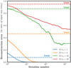 |
Fig. 2 Convergence speed of the GS algorithm. The GS algorithm was applied for input turbulent screens for four different seeing conditions. The dashed lines represent the corresponding reconstruction error in the linear framework and the x-axis is given in log-scale. |
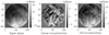 |
Fig. 3 Example of phase reconstruction with the nonmodulated PWFS. Left: input turbulent phase for D/r0 = 32, projected on the first 500 Zernike modes. Middle: linear reconstruction. Right: GS reconstruction after 2000 iterations. |
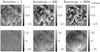 |
Fig. 4 Top: wrapped phases reconstructed by the GS algorithm. Bottom: corresponding unwrapped phases. |
3.2 Linearity curves and plots of the dynamic range
To achieve a more quantitative comparison in terms of the dynamic range between the linear and the GS reconstructors, linearity curves for some Zernike modes were analyzed. Zernike modes within a full range of amplitudes were sent through the PWFS and were then reconstructed for four different cases: (i) nPWFS with a linear reconstructor (ii) modulated PWFS with a modulation radius of 3λ/D as a comparison point in terms of dynamic range, (iii) nPWFS with a GS reconstructor without the unwrapping step, and (iv) nPWFS with a GS reconstructor with phase unwrapping.
The results for four different Zernike modes ranging from low to high spatial frequency (Z6, Z19, Z150, and Z490) are plotted in Fig. 5. In this case, the GS reconstructor was used with an arbitrary number of 25 iterations (the impact of the number of iterations is assessed below). These linearity curves show the well-known behavior of the modulated PWFS with respect to the nPWFS: the increase in dynamic range for low-order modes located within the modulation radius is significant, and the dynamic range for high-order modes composed of spatial frequencies outside the modulation radius is comparable. The GS algorithm without the unwrapping algorithm shows an extended linear range for all the modes, but the response curves drop steeply after 1 rad rms of aberrations. This corresponds to the amplitude for which the phase starts to wrap (PtV greater than 2π), and therefore, the reconstructed phase starts to have a different shape from the unwrapped phase and the projection on Zernike modes is modified as more high-order modes are introduced. However, adding the unwrapping step to the reconstruction allows us to improve the linearity curves after 1 rad rms of input phase. It is clearly demonstrated here that the GS reconstructor with the unwrapping step allows us to significantly increase the nPWFS dynamic range for all modes.
For the plots in Fig. 5, it was arbitrarily chosen to run 25 iterations for the GS algorithm. The impact of the number of iterations on the linearity curve of the Zernike mode Z19 is assessed in Fig. 6, where the linearity curve for this mode is shown using 1, 25, and 200 iterations when the GS algorithm is combined with the unwrapping step. For one iteration, the linearity curve does not follow the y = x slope around a null phase. This shows that even in a small-phase regime, only one iteration of the algorithm is not enough to accurately recover the phase. We note that two 2 iterations are enough in the small-phase regime (in the ideal case of these simulations, where there is no model error). As expected, the linearity curves then improve with the number of iterations, especially for the strong-aberration regime.
The linearity curves provided in Figs. 5 and 6 partially demonstrate the gain in dynamic range because they do not evaluate the potential nonlinear cross talk between modes during reconstruction. Another approach to show the improved dynamics offered by the GS reconstructor is to generate dynamic range plots as proposed in Lin et al. (2022). In this method, we randomly introduced sampled aberrations based on Von Karman atmospheric power spectral density (PSD) into the PWFS system and vary the total wavefront error from 0 to 3 rad rms. For each wavefront error value, we injected and reconstructed 100 phase screens. This process was repeated for the nPWFS with the linear reconstructor, the GS algorithm with unwrapping (25 and 200 iterations), and the modulated PWFS (rmod = 3 λ/D). The mean values of the 100 reconstructions for each input amplitude for all configurations are plotted in Fig. 7. The figure reveals that the GS algorithm outperforms the linear reconstructor for the nPWFS. When we consider a satisfying reconstruction threshold as the point where reconstruction error reaches 10% of the input rms, then the GS algorithm extends the linearity range by a factor of approximately 3. Moreover, it achieves a dynamic performance comparable to the 3 λ/D modulated PWFS for input wavefront errors of up to 1.5 rad rms for 25 GS iterations and up to 2.3 rad rms for 200 GS iterations. For this test, the modulated PWFS shows the best linearity as expected from the analysis of the linearity curves presented Fig. 5: the modulated PWFS has the best dynamic range for low-order modes (which are affected by the modulation), and the input turbulent phases used to produce the curves in Fig. 7 have a higher amplitude for low-order modes.
We demonstrated that the GS algorithm combined with an unwrapping step can drastically improve the nPWFS dynamic range. Hence, it is possible to use this technique for reconstructing larger amplitude phases more accurately. Still, it is important to analyze the noise propagation through this reconstructor with respect to the linear framework because one of the motivations to use the nPWFS is the better sensitivity with respect to noise.
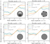 |
Fig. 5 Linearity curves for different Zernike modes, ranging from low to high order. The GS algorithm is run with 25 iterations in this case. |
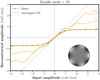 |
Fig. 6 Linearity curves for the Zernike mode 19 for different numbers of iterations while performing the GS algorithm. The number of iterations is written in the top right part of the curves. |
3.3 Noise propagation through reconstruction
To investigate the way in which noise spreads across different reconstructors, the four configurations outlined in the preceding section were used: an nPWFS with a linear reconstructor, a modulated PWFS, an nPWFS with a GS reconstructor without phase unwrapping, and an nPWFS with a GS reconstructor combined with phase unwrapping. For this study, only photon noise propagation was analyzed because it is a fundamental noise that cannot be mitigated by technological improvement. The effect of noise propagation was simply evaluated by introducing noise into the measurements and reconstructing the signals considering the different reconstructors. Once again, the idea is not to run an extensive simulation study on noise propagation through the GS algorithm in order to assess a large parameter space, but rather to highlight the basic sensitivity performance of this reconstructor with respect to the nPWFS and the modulated PWFS. To keep the analysis relatively simple, we studied two configurations: noise impact on the reconstruction of a flat wave-front (often referred to as reference intensities), and in the case of a turbulent phase screen with an amplitude of 0.75 radians rms (this is beyond nPWFS linearity range, but low enough to ensure that phase is not wrapped). To assess the noise propagation relative to these configurations, the following procedure was used in the simulation: for a given number of photons available for the measurement, the mean variance of each mode after reconstruction was estimated by averaging the variance of the reconstructed modes over 200 noise realizations. This operation was repeated for different numbers of photons, setting the number of iterations in the GS algorithm to 25. This number of iterations was once again arbitrarily chosen because we found that the number of iterations does not change the impact of the noise propagation.
The phase reconstruction errors due to photon noise propagation in the case of a flat wavefront and a 0.75 radians rms turbulent screen with respect to the incident flux are plotted in Fig. 8. The incident flux is expressed as the total number of photons available for measurements assuming a prefect transmission and a quantum efficiency of one for the detector (as a reminder, the reconstruction was performed over 500 Zernike modes).
For the cases of the linear reconstructor and a flat wavefront, Fig. 8 (top) shows a well-known behavior: the phase estimation error due to noise propagation through the reconstructor is lower for the nPWFS than for the modulated one. In the case of the GS algorithm, noise propagation behaves differently whether the unwrap step is performed or not.
In the context of noisy measurements for a flat wavefront, when unwrapping is omitted, the GS algorithm still propagates more error than the nPWFS and modulated PWFS for the high-flux regime, and it seems to perform slightly better than the modulated PWFS for the low-flux regime. For even lower flux regimes (not shown here), GS would even appear to perform better than the linear nPWFS reconstructor, but this behavior is misleading, in the sense that the GS algorithm always provides wrapped measurements, which prevents the amplitude of the reconstructed phase from diverging for extremely noisy measurements. Another way to explain this fact is to say that the GS has an intrinsic regularization that biases the results in this analysis. When the wrapping step is added, the GS reconstructor builds more error in the presence of noise compared to all the other configurations we studied.
Figure 8 provides the same analysis of the noise propagation for the case of a turbulent phase screen (0.75 nm rms). The same trend is visible, but there is an offset for the linear nPWFS reconstructor that corresponds to the reconstruction due to non-linearity error (which is absent for GS cases or the modulated PWFS).
To better understand the noise propagation behavior, it is useful to examine how the error propagates along the modes for one flux regime. An example is given Fig. 9 for the case of 400 photons per mode. The unwrapping step clearly drives the noise to drastically propagate on the low-order spatial frequencies.
To conclude this brief study of noise propagation, the GS reconstructor combined with an unwrapping algorithm performs poorly in the presence of noise because it propagates more noise than the modulated PWFS itself. Therefore, the sensitivity advantage of the nPWFS is lost while using this reconstructor. However, this implementation is currently in its most basic form. Noise propagation could be mitigated in the reconstructor through two aspects: on the one hand, by using a GS algorithm that is more robust against noise (Levin & Bendory 2019), and on the other hand, by using an unwrapping algorithm with a better behavior with respect to noise (Estrada et al. 2011). As mentioned in the introduction, using a nPWFS brings more advantages than only the gain in sensitivity with respect to noise, hence this current implementation of the reconstructor is still interesting for uses at high signal-to-noise ratio (S/N; application examples are given in the conclusion). It is also important to note that this drawback for the GS algorithm was not raised in previous studies that proposed its implementation to reconstruct the curvature of wavefront sensor signals (Guyon 2010).
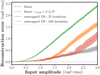 |
Fig. 7 Dynamic range plots produced by sending 100 randomly sampled phase screens following a Von Karman PSD for each input amplitude and reconstructing them. |
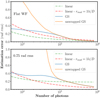 |
Fig. 8 Reconstruction errors due to photon noise. Top: case of an input flat wavefront. Bottom: case of an input turbulent wavefront of 0.756 radians rms. |
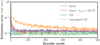 |
Fig. 9 Modal photon-noise propagation for 8000 photons for the measurements. |
3.4 Broadband impact on the performance
It is crucial to take into account the potential influence of larger spectral bandpass measurements on the GS algorithm when reconstructing the EM field, as this technique assumes the coherence of the field. The nPWFS is achromatic in phase (Fauvarque 2017), meaning that it measures the phase of the incoming wavefront independently of the wavelength of the light (dispersion effects are neglected here). However, the amplitude of the wavefront does depend on the wavelength because aberrations present in the system and the turbulence usually introduce a fixed optical-path difference (OPD) in all wavelengths. Hence, the measured signal will scale proportionally with the wavelength. This leads to two advantageous properties: for a flat wavefront, all the wavelengths will give the same measurements. In the right conditions, the closed loop can therefore converge towards a null phase. Second, by choosing the central wavelength for the reconstruction, it allows scaling of the phase to compensate for larger and smaller wavelengths, which returns a monochromatic measurement in the case of the linear range (providing a flat spectrum). Overall, it is known that the bandwidth has a limited impact on nPWFS measurements in general, and therefore, it seems reasonable to expect the same for the GS reconstructor, even though it assumes monochromatic measurements.
A thorough investigation of the broadband impact on reconstruction would require an extensive study assessing various factors such as the amplitude of the measured phase, the sampling used for the measurements, and the bandwidth. Because the scope of this paper is limited, a brief example is given to illustrate the impact of a broadband measurement on the GS algorithm using the same configuration as in the previous section, but providing the algorithm measurements recorded by a polychromatic light with a flat spectrum ranging from 550 nm to 800 nm (bandwidth about 35%, sampled with 50 points in our simulation). To run the GS algorithm, the nPWFS model was simulated as working at a monochromatic wavelength, set as the broadband central wavelength (675 nm). Linearity curves for Zernike mode 19 in the case of different numbers of GS iterations are again displayed, but adding the one corresponding to the reconstruction of a broadband measurement (Fig. 10). Figure 10 demonstrates the limited impact of the broadband measurement on the reconstruction, even though the chosen bandwidth is large.
To confirm the GS algorithm robustness to broadband measurement, the reconstruction error as a function of iteration number for a turbulent screen in the case D/r0 = 4 is plotted in Fig. 11. The reconstruction error stabilizes to a reconstruction error that is slightly larger than in the monochromatic case.
Overall, this short study points out that broadband measurements should not jeopardize the GS reconstruction scheme. We also mention that a polychromatic implementation of the GS algorithm could be imagined (Fienup 1999), but it will come at the expense of the computational time.
As the GS reconstruction scheme proposed in this paper is highly model dependent, it is important to show that our technique is robust enough to model errors, so that it can be implemented on a real experimental setup. This is shown in the next section, in which we provide an experimental demonstration of our reconstructor.
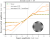 |
Fig. 10 Impact of a broadband measurement on the linearity curves for Zernike mode 19. |
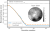 |
Fig. 11 Impact of a broadband measurement on the phase reconstruction. The input phase is the turbulent screen for D/r0 = 4 (color bar in radians). |
4 Experimental demonstration
4.1 Experimental setup
The goal of this section is to present a laboratory demonstration of the GS algorithm on SEAL, an extreme adaptive optics testbed composed of several deformable mirrors (DM), wave-front sensors, and coronagraphic branches. A schematic layout of the SEAL testbed for the nPWFS subsystem alone is presented in Fig. 12. The SEAL components relevant for the experiment described here are the source at λ = 635 nm, spatial light modulator (SLM) with 1100 pixels across the pupil diameter (van Kooten et al. 2022), an IRISAO segmented deformable mirror (DM) has six segments across the pupil diameter, a low-order ALPAO DM has nine actuators across the pupil diameter and a high-order BMC DM has 24 actuators across the pupil diameter. The focal-plane camera is sampled at 2.3 Shannon and the nPWFS is composed of a double-rooftop mask (Lozi et al. 2019) with 106 pixels across the pupil diameter on the camera (same sampling as the simulations reported in this paper).
To build a reliable model of the SEAL nPWFS and run the GS algorithm, two quantities are required: an image of the pupil, and the shape of the pyramid mask. To obtain an image of the pupil, large tip-tilt offsets were applied on the ALPAO DM in order to move the PSF away from the pyramid tip (~20λ/D) and place it successively in each nPWFS quadrant. By doing so, four images of the pupil were obtained through each side of the pyramid mask. The SEAL pupil was then computed by recentering and averaging these four images, with an estimated accuracy below one pixel. An image of the SEAL pupil measured through this method is shown in the top left panel of Fig. 1. The segments gaps created by the IRISAO DM are clearly visible. In order to compute the pyramid shape, the four pupil images were simply registered in order to produce the corresponding tip-tilt for each face of the pyramid mask. The phase-to-DMs (ALPAO and BMC) registration was made the following way: the central actuator of the DM was pushed and reconstructed, and then again pulled and reconstructed. The difference of the images corresponds to the phase of this actuator. Then a waffle pattern was sent to the DM and was reconstructed in order to register the actuator positions. Finally, the phase of the central actuator was fitted with a Gaussian function and was duplicated at the other actuatos positions. This calibration process requires only four images (two for the central actuator, and two for the waffle). For the ALPAO and BMC DM, the reconstructed phase is largely oversampled (106 pixels across versus 23 actuators for the BMC). The nPWFS and associated GS algorithm are routinely used on the SEAL testbed with both DMs as the standard way to flatten the wavefront in order to correct for quasi-static aberrations, achieving a wavefront error of about 17 nm rms (as measured by the nPWFS).
The nPWFS image after the closed loop is shown in Fig. 13 (left). A high-frequency pattern caused by the BMC DM is clearly visible (a well-known effect, called the print-through or quilting effect). The corresponding residual phase was reconstructed from the reference image (best flat after the closed loop on static aberrations) and propagated in the model. The obtained image is displayed in Fig. 13 (right), showing that the model exhibits high fidelity with the measurements. The small differences that can be spotted include the print-through effect, which seems slightly underestimated in the simulated image most likely because the field of view of the simulated nPWFS is smaller than the real one, which acts like a spatial low-pass filter), and a faint ring pattern can be seen between the two bottom pupil images of the true image (most likely caused by a dust particle on the glass pyramid). It is worth mentioning that all the results presented in the following subsections were obtained for measurements made at high S/N.
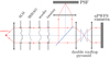 |
Fig. 12 Simplified layout of the SEAL testbed for the nPWFS subsystem. |
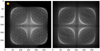 |
Fig. 13 Flat wavefront on the SEAL nPWFS. Left: nPWFS image on SEAL after the closed loop. The nPWFS estimated wavefront error is 17 nm rms. Right: corresponding simulated image. The same scaling is used for both images. |
4.2 Linearity curves
As a first demonstration of the GS algorithm performance on the SEAL testbed, some of the linearity curves obtained in the simulations in the previous section are reproduced. This study was made in the following way: Zernike modes were sent with the SLM to gain a good knowledge value of the input phase. Following the same procedure as before, the linear reconstructor was calibrated with the Zernike modal basis, hence the reconstruction directly gives the value of each of the modes. For the GS algorithm, the phase was reconstructed for each pixel and was then projected on the Zernike basis.
The linearity curves obtained for the Zernike mode 19 and 150 are shown in Fig. 14 for the 200 iterations we used for the GS algorithm. The conclusions from the simulations are confirmed in this experiment: the GS demonstrates a higher dynamic range than the linear reconstructor. However, for higher-order modes, the GS algorithm without phase unwrapping seems to under-perform compared to the simulation (Fig. 5). This could be explained by model errors that affect the performance slightly.
4.3 Example of phase reconstruction and close loop
As a demonstration of the GS capabilities in reconstructing strong phase aberrations on the bench, a D/r0 = 32 phase screen was generated on the SLM (bottom left panel of Fig. 15). The corresponding recorded nPWFS image is shown in the top left panel of the same figure, and the reconstructed unwrapped phase after 200 iterations is displayed in the bottom right corner. Figure 15 also shows a simulated image of the nPWFS signal, produced by simply propagating the reconstructed phase in the nPWFS model. Although the simulated and the real image are almost identical, the phase is largely underestimated (by more than a factor of 2; this effect was also observed in the simulations presented in the previous section). This is explained by the fact that the nPWFS saturates: for an increasing input phase, the signal reaches a point at which it almost does no longer change. A simple example of this saturation is the case of a tip-tilt aberration: when the PSF is moved several tens of λ/D in one quadrant, only one pupil image of the nPWFS is illuminated. Displacing the PSF even farther away will almost have no impact on the measurements because the illuminated pupil image already concentrates the entire flux. The saturation is a strong effect that will limit the reconstruction range for any type of linear but also nonlinear reconstructor because it implies that two different phases can lead to the same measurements. Hence, the saturation seems to be an intrinsic limitation in the nPWFS measurement, and inverting large-amplitude aberrations more accurately would require additional knowledge of the phase to be measured. A potential solution to even further improve the dynamic range of GS reconstruction is sketched in the next section.
Reconstructed phases at different iteration steps are displayed in Fig. 16. As shown before, the phase estimation improves with iterations, but the estimation appears to stop improving after just aa few hundred iterations instead of a few thousand iterations in the simulations. Hence, the reconstructed phases for 200 and 2000 iterations are highly similar. Once again, this could be explained by the differences between the nPWFS on the SEAL testbed and its model used for reconstruction.
It is also possible to compare the GS reconstruction with the linear reconstruction. To do this, a push-pull interaction matrix was measured on the bench by sending the first 500 Zernike modes on the SLM. The command matrix was then computed by taking the pseudo-inverse of the interaction matrix, and it was used to reconstruct the signal. The comparison between the linearly reconstructed phase and the GS reconstructed unwrapped phase projected on the first 500 Zernike modes is shown in Fig. 17. Our GS reconstruction clearly also shows a significant improvement compared to the linear reconstruction on the bench.
To conclude the testbed demonstration, we present results of a closed-loop run using the BMC DM (controlling all the modes) on the static turbulent screen presented in Fig. 15. The linear reconstructor uses a push-pull zonal interaction matrix, and the GS reconstructor uses 25 iterations with phase unwrapping. For the closed-loop AO control, a simple integrator controller with a loop gain of 0.5 was used. The PSFs obtained after 12 closed-loop steps are presented in Fig. 18. In the figure, we also present the PSF corresponding to the best flat after closing the loop with the nPWFS on bench aberrations (with the BMC DM), and the uncorrected PSF corresponding to the atmospheric phase displayed on the SLM. The best flat PSF exhibits a faint and vertical light pattern that crosses its core. This comes from diffraction effects due to the SLM. The closed-loop test clearly confirms the extended dynamic range of our reconstructor by showing that the closed loop with the GS reconstructor outperforms the closed loop in the linear framework (which finally diverges after a few dozen steps). It also shows that despite saturation effects, the AO closed-loop scheme helps to correct the high-amplitude phase with the nPWFS combined with the GS algorithm. As the wavefront error drastically improved after bootstrap, we could imagine a closed-loop scheme for which the number of GS iterations used for the reconstruction is reduced in the residual-phase regime.
These experimental tests demonstrate the GS reconstructor performance on an optical bench. They show that it provides an improvement over the linear reconstructor.
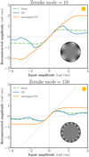 |
Fig. 14 Top: linearity curve for Z19 obtained on SEAL. Bottom: linearity curve for Z150 obtained on SEAL. The GS algorithm is used with 200 iterations. The yellow dots highlight the fact that these curves were obtained on the SEAL testbed. |
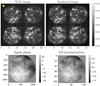 |
Fig. 15 Comparison of nPWFS signals from SEAL and simulated ones in presence of turbulence. Top-left: nPWFS image on the SEAL testbed. Top right: nPWFS simulated image (propagating the reconstructed phase through the nPWFS model). Bottom left: input phase on the SLM. Bottom right: reconstructed unwrapped phase with 200 iterations for the GS algorithm. |
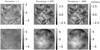 |
Fig. 16 Phases reconstructed for 1, 200, and 2000 iterations. Top: wrapped phases reconstructed by the GS algorithm on SEAL. Bottom: corresponding unwrapped phases. |
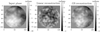 |
Fig. 17 Left: input turbulent phase injected on the SLM for D/r0 = 32, projected on the first 500 Zernike modes. Middle: linear reconstruction. Right: GS reconstruction after 2000 iterations. |
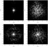 |
Fig. 18 Closing the loop with the BMC DM on a static atmospheric screen. Top left: PSF corresponding to best flat on the SEAL testbed. Top right: uncorrected PSF for an input phase D/r0 = 32 on the SLM. Bottom left: PSF after 12 closed-loop steps using the GS reconstructor. Bottom right: PSF after 12 closed-loop steps using the linear reconstructor. |
5 Beyond the nonmodulated PWFS saturation
As described in the previous section, the dynamic range of the GS algorithm seems to be limited by the saturation of the nPWFS measurements. As we showed, we can find different phases (in our case, the same shape, but different amplitudes) that substantially provide the same measurements on the nPWFS. Therefore, high-amplitude input phases cause a degeneracy in the measurements that seems to be unsolvable, regardless of which nonlinear reconstructor is considered. To push the dynamic range further, additional information about the phase is needed. To obtain this, the following strategy is proposed: a second sensor that would be a focal-plane camera located just before the pyramid tip, as shown in the schematic in Fig. 19.
The technique to use a focal-plane image in order to push PWFS dynamics has already been proposed in Chambouleyron et al. (2021). Here, the PSF image delivered by this camera provides the amplitude of the EM field in the focal plane, allowing this additional information to be added in the GS algorithm procedure. The information of the EM amplitude recorded at the focal plane can be used to replace the simulated focal-plane EM-field amplitude during back-propagation (between steps 1 and 2 in Fig. 1) and during forward-propagation (between steps 3 and 4 in Fig. 1). To do this, the simulated amplitude of the EM-field at the PWFS apex is replaced by the square root of the PSF measurement, while the simulated EM phase is kept. We call this reconstruction the focal-plane-assisted GS (f-GS).
The f-GS reconstructor was tested in a simulation with the same system as in Sect. 3, using as input phase the atmospheric screen used in Fig. 15 (case D/r0 = 32). For this input phase, a convergence plot similar to Fig. 2 is presented in Fig. 20 for the GS reconstructor and the f-GS reconstructor (both being unwrapped). The f-GS outperforms the standard GS algorithm in two ways: first, the convergence speed is much faster, and only one iteration is enough to provide a decent phase reconstruction. This represents a significant improvement because it could allow the GS approach to potentially be used in real time. Second, the overall reconstruction is also improved, showing that this strategy is indeed a solution to push the reconstruction further than the nPWFS saturation. The corresponding reconstructed unwrapped phases after one iteration and 4000 iterations for the GS and f-GS are shown in Fig. 21. The figure shows that after only one iteration, the f-GS reconstructed phase is already similar to the input phase, whereas the GS phase is largely underestimated (f-GS provides a three times better reconstruction error in the first iteration). Even after 4000 iterations, the GS algorithm does not provide a better phase estimation than the f-GS after one iteration.
Hence, the f-GS could be a powerful tool for drastically increasing the convergence speed of the algorithm and performance in the case of high amplitude aberrations. These advantages come with a more complicated practical implementation, requiring splitting the flux (an operation that could introduce noncommon-path aberrations) between two synchronized cameras. The details of this implementation will be considered in future studies, with the main motivation of building a demonstration of the f-GS on the SEAL testbed. We note that f-GS may not be needed in the case of a classic AO closed-loop scheme because the nPWFS would work around residual phases and therefore far from the saturation regime after bootstrap is completed. Nevertheless, this f-GS setup could open the nPWFS to a wider range of applications that would require performing wavefront sensing on large phases.
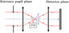 |
Fig. 19 Focal-plane assisted GS algorithm for the nPWFS. |
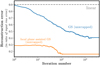 |
Fig. 20 Simulated convergence plot for an input atmospheric phase for D/r0 = 32. |
 |
Fig. 21 Reconstructed phases for the f-GS compared to the standard algorithm for one iteration and 4000 iterations. All phases are displayed with the same scaling. |
6 Conclusion
We introduced a new way to invert the nPWFS measurements that relies on the numerical model of the sensor and on the use of the GS algorithm. We demonstrated that the GS-based reconstructor along with an unwrapping algorithm can drastically improve the nPWFS dynamic range of the reconstruction compared to the linear framework and can extend its linearity range by a factor of approximately 3. Moreover, it can achieve a dynamic performance comparable to the 3 λ/D modulated PWFS up to 2 rad rms. This technique was successfully demonstrated on the SEAL testbed at UCSC, on which it was used to close the loop on high D/r0 turbulent phase screens. This reconstructor has two drawbacks, however: it is highly computationally complex, which prevents it from being used for real-time control purposes (in its current implementation), and the noise propagation is worse compared to the linear reconstructor. However, noise propagation for only the most basic implementation of GS and phase unwrapping was studied in this paper. There might be a better-suited GS algorithm combined with a noise-robust phase-unwrapping algorithm that could improve the noise propagation. The GS reconstructor already has several areas that can be useful in an AO system even though they were only tested at high S/N at slow speeds. For example, calibration purposes (as done routinely on the SEAL testbed), segment or fragment phasing, or highly sampled phase reconstruction. It could also support a second-stage nPWFS running in real time with a linear reconstructor through soft real-time reconstruction of the phase in order to compute optical gains, and it might also be used to reconstruct telemetry data with higher fidelity.
The most promising path toward a real-time implementation of this technique is to use focal-plane-assisted GS, which we showed in the simulation in Sect. 5. This technique uses the fact that the GS algorithm is well suited for sensor fusion and seems to significantly increase the convergence speed of the algorithm while allowing us to measure high-amplitude phases with better accuracy. The next steps for this approach is to push our understanding of the f-GS and start to implement it on the SEAL testbed, using a PSF image as an additional sensor.
Finally, the GS algorithm was applied in this paper for nPWFS alone, but we argue that it can be used for all Fourier-filtering WFS and maybe beyond. In a more general way, this reconstructor belongs to a wider class of reconstructors that use a numerical model of the sensor and iterative algorithms to increase the dynamic range.
Acknowledgments
This work was performed under the auspices of the U.S. Department of Energy by Lawrence Livermore National Laboratory under Contract DE-AC52-07NA27344. The document number is LLNL-JRNL-850197.
References
- Archinuk, F., Hafeez, R., Fabbro, S., Teimoorinia, H., & Véran, J.-P. 2023, arXiv e-prints [arXiv:2305.09805] [Google Scholar]
- Bertrou-Cantou, A., Gendron, E., Rousset, G., et al. 2022, A&A, 658, A49 [NASA ADS] [CrossRef] [EDP Sciences] [Google Scholar]
- Chambouleyron, V., Fauvarque, O., Janin-Potiron, P., et al. 2020, A&A, 644, A6 [EDP Sciences] [Google Scholar]
- Chambouleyron, V., Fauvarque, O., Sauvage, J. F., Neichel, B., & Fusco, T. 2021, A&A, 649, A70 [NASA ADS] [CrossRef] [EDP Sciences] [Google Scholar]
- Chanan, G., Troy, M., Dekens, F., et al. 1998, Appl. Opt., 37, 140 [NASA ADS] [CrossRef] [Google Scholar]
- Demers, R., Bouchez, A., Quiros-Pacheco, F., et al. 2022, in Adaptive Optics Systems VIII, 12185, eds. L. Schreiber, D. Schmidt, & E. Vernet, International Society for Optics and Photonics (SPIE), 1218518 [Google Scholar]
- Deo, V., Gendron, É., Rousset, G., et al. 2019, A&A, 629, A107 [NASA ADS] [CrossRef] [EDP Sciences] [Google Scholar]
- Estrada, J. C., Servin, M., & Quiroga, J. A. 2011, Opt. Express, 19, 5126 [NASA ADS] [CrossRef] [Google Scholar]
- Fauvarque, O. 2017, PhD thesis, Astrophysique et cosmologie Aix-Marseille, France [Google Scholar]
- Fienup, J. R. 1982, Appl. Opt., 21, 2758 [NASA ADS] [CrossRef] [Google Scholar]
- Fienup, J. R. 1999, J. Opt. Soc. Am. A, 16, 1831 [NASA ADS] [CrossRef] [Google Scholar]
- Frazin, R. A. 2018, J. Opt. Soc. Am. A, 35, 594 [NASA ADS] [CrossRef] [Google Scholar]
- Frigo, M. 1999, SIGPLAN Not., 34, 169 [CrossRef] [Google Scholar]
- Gerchberg, R. W. 1972, Optik, 35, 237 [Google Scholar]
- Ghiglia, D. C., & Romero, L. A. 1994, J. Opt. Soc. Am. A, 11, 107 [NASA ADS] [CrossRef] [Google Scholar]
- Guyon, O. 2005, ApJ, 629, 592 [NASA ADS] [CrossRef] [Google Scholar]
- Guyon, O. 2010, PASP, 122, 49 [NASA ADS] [CrossRef] [Google Scholar]
- Hutterer, V., Neubauer, A., & Shatokhina, J. 2023, Inverse Probl., 39, 035007 [NASA ADS] [CrossRef] [Google Scholar]
- Jensen-Clem, R., Dillon, D., Gerard, B., et al. 2021, SPIE Conf. Ser., 11823, 118231D [NASA ADS] [Google Scholar]
- Korkiakoski, V., Vérinaud, C., & Louarn, M. L. 2008, in Adaptive Optics Systems, 7015, eds. N. Hubin, C. E. Max, & P. L. Wizinowich, International Society for Optics and Photonics (SPIE), 1422 [Google Scholar]
- Kunkel, J. M., Yokota, R., Balaji, P., & Keyes, D. 2017, High Performance Computing (Springer International Publishing) [CrossRef] [Google Scholar]
- Landman, R., & Haffert, S. Y. 2020, Opt. Exp., 28, 16644 [NASA ADS] [CrossRef] [Google Scholar]
- Levin, E., & Bendory, T. 2019, arXiv e-prints [arXiv:1911.13179] [Google Scholar]
- Lin, J., Fitzgerald, M. P., Xin, Y., et al. 2022, J. Opt. Soc. Am. B, 39, 2643 [NASA ADS] [CrossRef] [Google Scholar]
- Lozi, J., Jovanovic, N., Guyon, O., et al. 2019, PASP, 131, 044503 [NASA ADS] [CrossRef] [Google Scholar]
- Nousiainen, J., Rajani, C., Kasper, M., et al. 2022, A&A, 664, A71 [NASA ADS] [CrossRef] [EDP Sciences] [Google Scholar]
- Por, E. H., Haffert, S. Y., Radhakrishnan, V. M., et al. 2018, SPIE Conf. Ser., 10703, 1070342 [NASA ADS] [Google Scholar]
- Ragazzoni, R. 1996, J. Mod. Opt., 43, 289 [Google Scholar]
- Ragland, S., Jolissaint, L., Wizinowich, P., et al. 2016, in Adaptive Optics Systems V, 9909, eds. E. Marchetti, L. M. Close, & J.-P. Véran, International Society for Optics and Photonics (SPIE), 99091P [Google Scholar]
- Schwartz, N., Sauvage, J.-F., Correia, C., et al. 2017, in Proceedings of the Adaptive Optics for Extremely Large Telescopes 5 (Instituto de Astrofisica de Canarias (IAC)) [Google Scholar]
- van Kooten, M. A. M., Jensen-Clem, R., Fowler, J., et al. 2022, in Adaptive Optics Systems VIII, 12185, eds. L. Schreiber, D. Schmidt, & E. Vernet, International Society for Optics and Photonics (SPIE), 121856V [Google Scholar]
- Vérinaud, C. 2004, Opt. Commun., 233, 27 [Google Scholar]
All Figures
|
Fig. 1 Principle of the GS algorithm applied to nonmodulated PWFS. The yellow dots highlight the fact that these are true data obtained on the SEAL testbed. |
| In the text | |
|
Fig. 2 Convergence speed of the GS algorithm. The GS algorithm was applied for input turbulent screens for four different seeing conditions. The dashed lines represent the corresponding reconstruction error in the linear framework and the x-axis is given in log-scale. |
| In the text | |
|
Fig. 3 Example of phase reconstruction with the nonmodulated PWFS. Left: input turbulent phase for D/r0 = 32, projected on the first 500 Zernike modes. Middle: linear reconstruction. Right: GS reconstruction after 2000 iterations. |
| In the text | |
|
Fig. 4 Top: wrapped phases reconstructed by the GS algorithm. Bottom: corresponding unwrapped phases. |
| In the text | |
|
Fig. 5 Linearity curves for different Zernike modes, ranging from low to high order. The GS algorithm is run with 25 iterations in this case. |
| In the text | |
|
Fig. 6 Linearity curves for the Zernike mode 19 for different numbers of iterations while performing the GS algorithm. The number of iterations is written in the top right part of the curves. |
| In the text | |
|
Fig. 7 Dynamic range plots produced by sending 100 randomly sampled phase screens following a Von Karman PSD for each input amplitude and reconstructing them. |
| In the text | |
|
Fig. 8 Reconstruction errors due to photon noise. Top: case of an input flat wavefront. Bottom: case of an input turbulent wavefront of 0.756 radians rms. |
| In the text | |
|
Fig. 9 Modal photon-noise propagation for 8000 photons for the measurements. |
| In the text | |
|
Fig. 10 Impact of a broadband measurement on the linearity curves for Zernike mode 19. |
| In the text | |
|
Fig. 11 Impact of a broadband measurement on the phase reconstruction. The input phase is the turbulent screen for D/r0 = 4 (color bar in radians). |
| In the text | |
|
Fig. 12 Simplified layout of the SEAL testbed for the nPWFS subsystem. |
| In the text | |
|
Fig. 13 Flat wavefront on the SEAL nPWFS. Left: nPWFS image on SEAL after the closed loop. The nPWFS estimated wavefront error is 17 nm rms. Right: corresponding simulated image. The same scaling is used for both images. |
| In the text | |
|
Fig. 14 Top: linearity curve for Z19 obtained on SEAL. Bottom: linearity curve for Z150 obtained on SEAL. The GS algorithm is used with 200 iterations. The yellow dots highlight the fact that these curves were obtained on the SEAL testbed. |
| In the text | |
|
Fig. 15 Comparison of nPWFS signals from SEAL and simulated ones in presence of turbulence. Top-left: nPWFS image on the SEAL testbed. Top right: nPWFS simulated image (propagating the reconstructed phase through the nPWFS model). Bottom left: input phase on the SLM. Bottom right: reconstructed unwrapped phase with 200 iterations for the GS algorithm. |
| In the text | |
|
Fig. 16 Phases reconstructed for 1, 200, and 2000 iterations. Top: wrapped phases reconstructed by the GS algorithm on SEAL. Bottom: corresponding unwrapped phases. |
| In the text | |
|
Fig. 17 Left: input turbulent phase injected on the SLM for D/r0 = 32, projected on the first 500 Zernike modes. Middle: linear reconstruction. Right: GS reconstruction after 2000 iterations. |
| In the text | |
|
Fig. 18 Closing the loop with the BMC DM on a static atmospheric screen. Top left: PSF corresponding to best flat on the SEAL testbed. Top right: uncorrected PSF for an input phase D/r0 = 32 on the SLM. Bottom left: PSF after 12 closed-loop steps using the GS reconstructor. Bottom right: PSF after 12 closed-loop steps using the linear reconstructor. |
| In the text | |
|
Fig. 19 Focal-plane assisted GS algorithm for the nPWFS. |
| In the text | |
|
Fig. 20 Simulated convergence plot for an input atmospheric phase for D/r0 = 32. |
| In the text | |
|
Fig. 21 Reconstructed phases for the f-GS compared to the standard algorithm for one iteration and 4000 iterations. All phases are displayed with the same scaling. |
| In the text | |
Current usage metrics show cumulative count of Article Views (full-text article views including HTML views, PDF and ePub downloads, according to the available data) and Abstracts Views on Vision4Press platform.
Data correspond to usage on the plateform after 2015. The current usage metrics is available 48-96 hours after online publication and is updated daily on week days.
Initial download of the metrics may take a while.