| Issue |
A&A
Volume 680, December 2023
|
|
|---|---|---|
| Article Number | A15 | |
| Number of page(s) | 19 | |
| Section | The Sun and the Heliosphere | |
| DOI | https://doi.org/10.1051/0004-6361/202347536 | |
| Published online | 04 December 2023 | |
Analysis of full-disc Hα observations: Carrington maps and filament properties in 1909–2022⋆
1
Max Planck Institute for Solar System Research, Justus-von-Liebig-Weg 3, 37077 Göttingen, Germany
e-mail: This email address is being protected from spambots. You need JavaScript enabled to view it.
2
INAF Osservatorio Astronomico di Roma, Via Frascati 33, 00078 Monte Porzio Catone, Italy
3
Aryabhatta Research Institute of Observational Sciences, Manora Peak, Nainital 263 001, India
4
Instituto de Astrofísica e Ciências do Espaço, University of Coimbra, R. do Observatório, 3040-004 Coimbra, Portugal
5
Department of Earth Sciences, University of Coimbra, R. Sílvio Lima, 3030-790 Coimbra, Portugal
6
Larissa Observatory “Aristeus”, Giannouli, 41500 Larissa, Greece
7
INAF Osservatorio Astrofisico di Catania, Via S. Sofia 78, 95123 Catania, Italy
8
Department of Physics, University of Coimbra, R. Larga, 3004-516 Coimbra, Portugal
9
National Astronomical Observatory of Japan, 2-21-1 Osawa, Mitaka, Tokyo 181-8588, Japan
10
Astronomical Institute of Kharkiv V.N. Karazin National University, 35 Sumskaya St., Kharkiv 61022, Ukraine
11
LESIA, Observatoire de Paris, 5 Pl. Jules Janssen, 92195 Meudon, France
12
PSL Research University, 60 Rue Mazarine, 75006 Paris, France
Received:
22
July
2023
Accepted:
16
September
2023
Abstract
Context. Full-disc observations of the Sun in the Hα line provide information about the solar chromosphere, and in particular, about the filaments, which are dark and elongated features that lie along magnetic field polarity-inversion lines. This makes them important for studies of solar magnetism. Because full-disc Hα observations have been performed at various sites since the second half of the 19th century, with regular photographic data having started at the beginning of the 20th century, they are an invaluable source of information on past solar magnetism.
Aims. We derive accurate information about filaments from historical and modern full-disc Hα observations.
Methods. We consistently processed observations from 15 Hα archives spanning 1909–2022. The analysed datasets include long-running ones such as those from Meudon and Kodaikanal, but also previously unexplored datasets such as those from Arcetri, Boulder, Larissa, and Upice. Our data processing includes photometric calibration of the data stored on photographic plates, the compensation for limb-darkening, and the orientation of the data to align solar north at the top of the images. We also constructed Carrington maps from the calibrated Hα images.
Results. We find that filament areas, similar to plage areas in Ca II K data, are affected by the bandwidth of the observation. Thus, a cross calibration of the filament areas derived from different archives is needed. We produced a composite of filament areas from individual archives by scaling all of them to the Meudon series. Our composite butterfly diagram very distinctly shows the common features of filament evolution, that is, the poleward migration as well as a decrease in the mean latitude of filaments as the cycle progresses. We also find that during activity maxima, filaments cover ∼1% of the solar surface on average. The change in the amplitude of cycles in filament areas is weaker than in sunspot and plage areas.
Conclusions. Analysis of Hα data for archives with contemporaneous Ca II K observations allowed us to identify and verify archive inconsistencies, which also have implications for reconstructions of past solar magnetism and irradiance from Ca II K data.
Key words: Sun: activity / Sun: chromosphere / Sun: filaments / prominences / astronomical databases: miscellaneous / Sun: rotation
The filament area butterfly diagram is available at the CDS via anonymous ftp to cdsarc.cds.unistra.fr (130.79.128.5) or via https://cdsarc.cds.unistra.fr/viz-bin/cat/J/A+A/680/A15
© The Authors 2023
 Open Access article, published by EDP Sciences, under the terms of the Creative Commons Attribution License (https://creativecommons.org/licenses/by/4.0), which permits unrestricted use, distribution, and reproduction in any medium, provided the original work is properly cited.
This article is published in open access under the Subscribe to Open model.
Open access funding provided by Max Planck Society.
1. Introduction
The first line of the hydrogen Balmer series at 6562.79 Å, known as Hα line, is one of the deepest and broadest lines of the visible spectrum of the Sun. Janssen (1869) and Lockyer & Frankland (1869) were the first to observe on-disc solar features in Hα. In the late 1800s, Secchi (Secchi 1871) and Tacchini (Tacchini 1872) made daily observations in the Hα line (Bocchino 1933; Ermolli & Ferrucci 2021; Ermolli et al. 2023), and even though these were regular observations, they were merely visual inspections and reported in drawings. At that time, Hα observations were not common, and it was not before the invention of the spectroheliograph (hereafter SHG, Hale 1904) and the daily use of photography that they could be explored more widely and systematically. Regular photographic observations in the Hα line started later than those in white light and the Ca II K line because the emulsion of the early photographic plates was not sensitive to wavelengths greater than ∼5900 Å. This changed with the invention of red-sensitized emulsions in 1907 (Wallace 1907), which allowed storing Hα observations on photographic plates since 1909. Therefore, Hα data make the third-longest series of direct photographic full-disc observations of the Sun after the white-light observations of the photosphere and Ca II K images of the chromosphere (Chatzistergos et al. 2022). Similarly to the Ca II K line, the Hα line has long been used as a tool for extracting information about the structure and dynamics of the solar chromosphere.
The Ca II K and Hα lines probe slightly different altitudes in the solar atmosphere (Vernazza et al. 1981). The wings and core of the Ca II K line almost continuously sample the heights from the photosphere to the high chromosphere, while the wings and core of the Hα line distinctly probe the deep photosphere and the overlying chromosphere, respectively. This distinct origin of the Ca II K and Hα results in a significantly different appearance of the chromosphere. While observations in the Ca II K line at 2 Å spectral resolution, for instance, mostly trace bright features associated with photospheric magnetic regions, Hα images show structures that mainly trace the canopy field in the higher atmosphere. When imaged at 2 Å spectral resolution, for instance Ca II K observations resemble unsigned magnetograms (Chatzistergos et al. 2019a; Murabito et al. 2023, and references therein) describing the evolution of the solar surface magnetic field in non-spot regions, while Hα data display a highly structured and dynamic environment filled with fibrils, mottles, filaments, and flaring regions (Carlsson et al. 2019).
Fibrils and mottles are short-lived (from a few minutes to a few hours), small-scale (of the order of tens of arcseconds) jet-like features that dominate the chromosphere above and about plage regions (De Pontieu et al. 2007) and in the quiet Sun, respectively. Their counterparts seen at the limb are known as spicules (e.g. Tsiropoula et al. 1994; Rouppe van der Voort et al. 2009; Pereira et al. 2012).
Filaments are long-lived (from days to weeks), large-scale (can reach up to lengths comparable to the solar radius; Mazumder et al. 2021) elongated structures of dense and relatively cold gas that appear dark relative to their surroundings in on-disc observations and bright when they protrude beyond the solar limb to form prominences (Parenti 2014). These structures, which are held in place by the magnetic field, lie between areas of opposite-polarity magnetic fields (Babcock & Babcock 1955; McIntosh 1972; Martin 1998). Prominences have been studied with Hα observations (e.g. Bocchino 1933; Carrasco et al. 2021, with such analyses extending information on prominences back to 1869 with observations by Respighi, Secchi, Tacchini, and Donati from Rome, Palermo, and Florence), and with disc-blocked or narrow-bandwidth Ca II K observations (e.g. Chatterjee et al. 2020; Carrasco & Vaquero 2022). Filaments can also be seen both in Hα and Ca II K observations, but they are less prominent in Ca II K data and can only be seen in observations acquired with relatively narrow bandwidths (e.g. as reported in the catalogues of the observatory of Coimbra between 1929–1944; Lourenço et al. 2021; Carrasco & Vaquero 2022; Wan & Li 2022). Therefore, most of the current knowledge on filaments comes from analyses of observations in the Hα line (e.g. Hansen & Hansen 1975; Makarov et al. 1982, 1983; Makarov & Sivaraman 1983; Coffey & Hanchett 1998; Mouradian 1998; Denker et al. 1999; Shih & Kowalski 2003; Fuller et al. 2005; Benkhalil et al. 2005; Zharkova & Schetinin 2005; Li et al. 2007; Yuan et al. 2011; Hao et al. 2013, 2015; Zou et al. 2014; Laurenceau et al. 2015; Tlatov et al. 2016; Chatterjee et al. 2017; Diercke & Denker 2019; Diercke et al. 2022; Lin et al. 2020; Suo 2020). It is worth noting that most of the previous studies were based on analyses of observations covering limited time intervals and archives. In particular, only the data from the Meudon and Kodaikanal observatories have been employed for periods before 1960. Moreover, previous studies based on analyses of multiple archives were mainly performed by appending results form the different series without studying potential inconsistencies of the data.
For a long time, these limitations, which also affected studies using observations at other wavelengths (e.g. Ca II K) were essentially imposed by the limited availability of data in digital form and the lack of the needed image-processing resources. However, over the recent years, these limitations have been superseded, allowing a more detailed and careful analysis of existing Hα data. Only an accurate and consistent analysis of multiple archives would allow accounting for artefacts in the results derived from the individual datasets and thus a meaningful assessment of the underlying solar processes (Ermolli et al. 2009a, 2018; Chatzistergos et al. 2019b, 2021). To achieve this goal, Chatzistergos et al. (2018a) introduced a novel approach to process full-disc solar observations from historical and modern series available in digital form (Chatzistergos 2017; Chatzistergos et al. 2016, 2018b, 2019b,c,d, 2020a,b). This approach, which includes an accurate photometric calibration of photographic observations and compensation for the centre-to-limb-variation (CLV), was found to return more accurate results than those achieved with other methods in the literature. Originally developed to analyse Ca II K data, this method can be applied to consistently process observations from multiple archives and in different spectral bands. In addition to 43 Ca II K datasets (Chatzistergos et al. 2020b), it has already been successfully applied to data over four continuum intervals (Chatzistergos et al. 2019a, 2020c; Ermolli et al. 2022) and provisionally to a small sample of Hα images from the Kanzelhöhe observatory (Asvestari et al. 2021).
Here, we analyse Hα data from 15 digitised archives to produce an extensive and consistent database of filaments covering the period 1909–2022. To our knowledge, this study substantially exceeds earlier similar efforts. Furthermore, 9 of the archives analysed in this study have not been used for such studies before, while the pre-1980 data from Meudon have previously only been analysed manually. Using multiple archives, we are able to increase the daily coverage of observations available for the analysis of filament evolution, and, even more importantly, to single out trends in the results that are not due to solar processes, but are rather introduced by changes in the instruments and characteristics of individual archives. Furthermore, for 12 of the analysed archives, there are near-co-temporal Ca II K observations from the same site. Thus our analysis of the Hα observations can also improve our understanding of the observational conditions for the Ca II K observations and vice versa.
The paper is structured as follows. The data and processing techniques are described in Sect. 2. We present the Carrington maps from the Hα observations and our results from the filament identification in Sect. 3. We summarise and draw our conclusions in Sect. 4. In Appendix A we compare the characteristics of the various archives.
2. Data and methods
2.1. Hα observations
We used full-disc Hα (6562.79 Å) observations from 15 archives. Table 1 lists the main characteristics of these archives. To our knowledge, the analysed archives comprise all historical datasets that are currently available in digital form, as well as some CCD-based ones that were available to us. In particular, we used the data from the Arcetri (Ar), Big Bear (BB), Boulder (Bo), Catania (CT), Coimbra (Co), Kanzelhöhe (Ka), Kharkiv (Kh), Kodaikanal (Ko), Larissa (La), McMath-Hulbert (MM), Meudon (MD), Mitaka (Mi), Pic du Midi (PM), Sacramento Peak (SP), and Upice (UP) observatories. Figure 1 shows exemplary images from all the analysed archives. In total, all these archives contain 182 073 images covering 36 991 days over the period 1909–2022. The temporal coverage is 89% over the entire period (which is between 19 April 1909, the first day with an Hα observation in our analysed archives, and 31 December 2022). The coverage is higher and rather stable at 99.7% since 1968, while it decreases steadily further back in time before 1968. Figure 2 gives the annual coverage from each archive separately and when all archives are combined together.
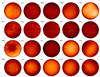 |
Fig. 1. Examples of Hα observations from the various archives analysed in this study. The images within each row correspond to the same day, with the exception of the Kh image (taken on 26 May 2000). In particular, the dates of the observations are 4 August 1965 for Ar, Ko, MD, MM, and Mi; 14 January 1980 for Bo, Ka, MD, and SP; 2 September 2011 for BB, Ka, La, Mi, and UP; and 13 September 2013 for BB, CT, Co, Ka, and PM. The images are shown after the pre-processing to identify the disc and to resample them to account for the disc ellipticity (when applicable) and convert the historical data to density values. The images have been aligned to show the solar north pole at the top. |
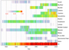 |
Fig. 2. Annual fractional coverage by the various Hα archives analysed in this study. The annual coverage by all the archives combined is shown as well. The annual coverage is colour-coded as shown by the colour bar plotted within the plot. The black boxes mark the years with complete daily coverage. |
Hα archives analysed in this study.
The archives analysed in this study include observations taken with diverse settings, while various instrumental changes potentially introduce inconsistencies in the series (similarly to what was reported for Ca II K data; Chatzistergos et al. 2022). They comprise observations performed with a spectroheliograph (Ar, Kh, Ko, MM, MD, SP, an Co) and optical filters (Mi, Bo, Ka, BB, CT, PM, La, and UP). The images were stored on photographic plates or film (Ar, Ko, MM, Bo, and SP) or taken with a CCD camera (BB, CT, PM, La, and UP), while the archives from Mi, Ka, Kh, MD, and Co include both CCD-based observations and those stored on photographic plates. Only a small sample of the Kh collection exists in digital form, which was scanned for the purposes of this study. Moreover, the Mi data used in this study derive from three different telescopes, that is, the Monochromatic Heliograph (1957–1992), the Automatic Flare Patrol Telescope (1991–2019), and the Solar Flare Telescope (since 2011). The data with the latter two telescopes were taken with a CCD camera, while those with the monochromatic heliograph were stored on films that were digitised in the late 1990s to early 2000s with 8-bit depth. Unfortunately, the films deteriorated and were eventually discarded, but they were fortunately first properly digitised. Since the filter used for the Automatic Flare Patrol Telescope severely degraded over the later years, we ignored the data taken with this filter since 2011. For this period, we only used the Mi data from the solar flare telescope. MD is the oldest Hα archive (Malherbe & Dalmasse 2019; Malherbe 2023), with the earliest observations dating back to 1909, and the full series currently covers ten solar cycles, while the one from La is the shortest series analysed in this study, covering less than one full solar cycle.
The datasets also differ in terms of observational cadence. Most currently running sites (BB, CT, and Ka) as well as Bo and Mi have high-cadence observations, while all other sites performed only a few observations per day. For our current analysis, we considered one to three images per day from the archives with high-cadence observations. An exception was Mi, for which we analysed all the data taken with the Automatic Flare Patrol Telescope (and a CCD camera) and approximately half of the available data taken with the Monochromatic Heliograph (and stored on photographic plates). This is because the Monochromatic Heliograph data were scanned in a way that most files include two solar observations, typically taken a few seconds apart. However, we still analysed one to three images per day from the Mi data taken with the Solar Flare Telescope. For the latter, we note that the archive includes data with three different exposures, of which we used the medium one to increase the signal-to-noise ratio. An exception was made for observations for which the medium exposure led to saturated plage regions, for which dates we used the low-exposure images. Another issue important for this study is the change from photographic plates to film in the Ko dataset in 1978 (Chatterjee et al. 2017). Unfortunately, most Ko photographs since 16 December 1998 appear to be torn, resulting in parts of the solar disc being missing in the observations. Notwithstanding this issue, we processed these data as well and still used them because they can provide information about filaments and plage regions away from the poles. We also corrected an inconsistency in the recording of the observational time of Ko data between 1 September 1942 and 15 October 1945, during which period daylight-saving time was used (Jha 2022).
The La data have not been described in the literature before. They were performed at the Larissa observatory1 in central Greece, which was founded by Nick Stoikidis in 1972. The telescope used for these observations has the following characteristics: the diameter of the objective lens is D = 160 mm, the focal length F = 2400 mm, and the focal ratio f/15. A CCD camera (PRO LINE PL11002M-2 by Finger Lakes Instrumentation) was used and produced images with dimensions of 4008 × 2672 pixel2. There are also more than 2000 35 mm film observations over 1991–1993, which have not yet been digitised, however.
2.2. Methods
All images were consistently processed with the methods developed by Chatzistergos et al. (2018a, 2019b, 2020b). Only the process with which we performed the photometric calibration of the photographic data was adapted to the specifics of the Hα line because there is a difference in the quiet-Sun (QS) centre-to-limb variation (CLV) in Ca II K and Hα observations. In the following, we briefly describe the applied processing.
As a first step, we identified the solar limb with a Sobel filtering followed by an ellipse fit to compute the coordinates of the disc centre and semi-major and minor axes (for more details, see Appendix B of Chatzistergos et al. 2019b, 2020a). This allowed us to account for the recorded solar disc ellipticity by resampling the images accordingly (Chatzistergos et al. 2020a,b). The background of the images, comprising the limb darkening and various small- and large-scale artefacts, was computed by applying a running-window median filter along with polynomial fitting across linear and radial segments (Chatzistergos et al. 2018a). This processing was applied iteratively such that the solar disc features were progressively excised to improve the accuracy of the background computation and eliminate the influence of bright and dark features in that computation. The relation between the QS CLV measured on the historical data and a reference QS CLV from CCD-based data allowed us to perform the photometric calibration for each image (only those stored in photographic plates) separately (see Chatzistergos et al. 2018a, for more details). As the reference QS CLV, we took that derived from Catania (CT) CCD-based observations over the period 2002–2018. The choice of the CT data as the reference was due to the sufficiently long interval of observations at that site, the high consistency of the data, the large number of daily observations per year, and the fact that this archive has a nominal bandwidth that is representative of most available Hα archives analysed here. We produced photometrically calibrated and limb-darkening-compensated contrast images with values given in the form of  , where Ci, j, Ii, j, and
  are the contrast, photometrically calibrated intensity, and photometrically calibrated intensity of QS for i, j pixel on the image. Thus, we note that contrast values are dimensionless.
Next, the images were rotated to align the solar north pole at the top side. For this purpose, the data were separated into three groups. The first group comprises the data from BB, CT, Ka, Ko, La, MM, Mi, PM, and UP for which the alignment was achieved by compensating for the ephemeris, that is, rotating the image by the p0 angle. However, for Ko, it was necessary to also account for the rotation of the coelostat, as was done by Jha (2022). The second group comprises most of the Ar, MD, and Co data, which were aligned prior to their digitisation. We note, however, that a 90° rotation was needed for the Ar data. The last group comprises the Kh, Bo, and SP data, which we aligned by using a cross-correlation approach. We used nearly cotemporal observations from other archives that were aligned as discussed previously to appropriately align the data from this third group. Data taken within a seven-day interval centred at the date of each observation were considered, but we selected the observation that was closest in time. Correction for the differential rotation was applied with SolarSoft routines (Freeland & Handy 1998), that is, to project the reference image to the time of the image that was to be aligned. When no observation from any other archive was found within that time frame, we used the observation that was closest in time from the same archive that was previously aligned to act as the reference. The cross-correlation approach was also used to validate the orientation of the data in the other two groups. This was done to verify whether the data in the second group were oriented correctly during the digitisation, but also because there might be errors in the date and time of observations, which would result in an incorrect orientation of the images (we recall that determination of the image rotation with ephemeris required accurate knowledge of the observations date and time). Observations for which the resulting angle with the cross-correlation technique deviated significantly from the previously defined angle were tagged as potentially incorrectly oriented, otherwise, the previously defined angle was used. The main reason for these errors was mistakes in the dating of the images, which thus allowed us to identify and correct incorrect observational dates and times in the various archives. We note, however, that large errors like this sometimes also occur because of differences between the two observations (e.g. large-scale artefacts that are not entirely accounted for, or image distortions). It is noteworthy that most Ko and SP data have markings on the plate to denote the orientation, which could be used to identify the poles. However, our approach allowed for better versatility, while we also identified mistakes in the placement of the markings of the observations.
Figure 3 shows the observations shown in Fig. 1 after their calibration to produce contrast images and after the image rotation to show the north pole at the top. Figure 3 demonstrates the effect on the observed solar features of several representative bandwidths used for acquisition of Hα data at various sites. In particular, the contrast of the plage and filament regions is greater for the narrow-band observations, for instance MD and SP, while they are fainter for broader-band observations, for instance Ka and Ko. We note that the contrast of features in the Co data is lower than that in MD, even though the nominal bandpass is roughly the same. This suggests that the Co data might have been taken slightly off-band or with a broader bandwidth compared to the MD ones. We note, however, that the transmission profile also affects the contrast. Furthermore, the information we have is about the nominal bandwidths, and the actual bandwidths can differ due to instrumental setups, but also, especially for the spectroheliograms, due to potential adjustments or tests made by the observers. This highlights the importance of having information about potential inconsistencies within the various archives. Appendix A presents information about the characteristics of the archives that allows assessing their homogeneity in time, such as the evolution of the disc eccentricity, large-scale inhomogeneities, spatial resolution, and a comparison between the measured CLV in the images to the average from CT data.
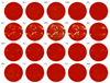 |
Fig. 3. Examples of photometrically calibrated and limb-darkening-compensated contrast images for the observations shown in Fig. 1. All images show contrast values in the range [ − 0.5, 0.5]. |
Finally, we identified filaments in all the processed observations by using a modification of the multiple-level tracking algorithm (Bovelet & Wiehr 2001). We applied two intensity thresholds (−3 and −5) as multiplicative factors to the standard deviation of the QS regions. This gave two separate sets of masks where the pixels with contrast values above each threshold have the value of unity, while the value of 0 was assigned to all remaining pixels. We then applied morphological operators to dilate and erode the mask obtained with the lower threshold. These operators were defined to have widths of fractions of the solar disc radius to render them consistent for all archives. We also applied a size threshold to the identified features to remove small-scale structures that were most likely artefacts. We kept only those features in the mask derived with the low contrast threshold that had at least one pixel in common with the features identified with the more conservative threshold. This processing, however, still detected spots (which generally appear diminished in Hα compared to continuum observations) as well as potential artefacts, such as scratches or hair introduced during the digitisation. In order to remove these artefacts and avoid mistakenly treating them as filaments, we applied a linear fit and an ellipse fit to the mask resulting from each identified region. This allowed us to exclude regions that were too circular, which are most likely spots, or segments that were too straight and thin, in which case they would most likely be artefacts. For a rather small number of images, this process results in oversegmentation and hence in an overestimation of filament areas. We identified and excluded these cases with a conservative upper threshold on disc-integrated filament areas of 10%. The pole markings were also removed from the SP data by removing all elongated vertical features found at the poles. Examples of masks with identified filaments are shown in Fig. 4.
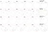 |
Fig. 4. Examples of masks identifying filaments in the observations shown in Fig. 1. The circles mark the disc boundaries, and filaments are shown in black. The last column is overlaid on the masks from the various observations taken on the same day and shown in the corresponding row in blue, red, green, yellow, and purple. The observations in each row were taken on the same day, with the exception of Kh in the second row, which is why it is not overlaid in the last panel of the row. In the masks shown in the last column, we have compensated for the differential rotation to show all of them as they would have been at 12:00 UTC. |
3. Results
Using the 15 Hα datasets (see Table 1) processed as described in the previous section, we produced Carrington maps and butterfly diagrams of filament areas. In the following, we present and discuss our results.
3.1. Carrington maps
Carrington maps are Mercator projections (Calabretta & Greisen 2002) of the entire solar surface over one solar rotation. We produced Carrington maps from all archives by considering only the regions within ±50° longitudes of each image. However, this approach can sometimes lead to gaps in the produced Carrington maps. We filled these gaps, to the degree possible, with the values from another Carrington map that was produced by considering the entire solar disc from each image. Overlapping images were averaged to produce the final maps.
Figure 5 shows examples of the Carrington maps we produced from nine archives that we analysed over three Carrington rotations. The comparison of images in Fig. 5 highlights the differences among the various archives. In particular, the Carrington map from Ar data exhibits higher contrast than the maps from Ko and MM of the same rotation. Similarly, filaments are more pronounced in Bo and CT Carrington maps than those for the same rotation from MD and Co, respectively. This might suggest that the observations taken with a very narrow bandwidth, such as those at MD and Co, might not be ideal for studying the filament evolution. However, we stress that archives such as Co and MD still allow performing quantitative studies of filaments.
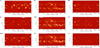 |
Fig. 5. Carrington maps constructed from the observations of nine Hα archives. Each column shows Carrington maps for the same rotations 1427 (7 May to 2 June 1960, left, see also the left column of Fig. 7), 1689 (30 November to 26 December 1979, middle), and 2141 (1 to 27 September 2013, right, see also the bottom row of Figs. 1–4). All maps show contrast values in the range [−0.5, 0.5]. |
The accuracy of the processing applied in our study is demonstrated by Fig. 6, which compares our Carrington maps based on Ko data to those by Chatterjee et al. (2017)2 and Lin et al. (2020)3. As representative examples, we show the Carrington maps for rotations 854 (23 July to 18 August 1917) and 1497 (29 July to 25 August 1965). The images over these intervals show many artefacts, mostly dark linear segments close to the limb. These artefacts are clearly visible in maps produced by Chatterjee et al. (2017) and Lin et al. (2020), while most of them are accounted for by our method. We note that the data artefacts cause filaments to be missed in the maps by Chatterjee et al. (2017) and Lin et al. (2020), for instance the filament for rotation 1497 for longitudes 300−360° in the northern hemisphere. However, we also note residual artefacts in the maps we produced that are absent in the maps by Chatterjee et al. (2017) and Lin et al. (2020), for example, the darker artefact for rotation 1497 for longitude 30° in the southern hemisphere. These are mostly small and clear artefacts close to the limb, which are magnified with their projection in this grid. These regions were removed in the maps by Chatterjee et al. (2017) and Lin et al. (2020) because the authors considered a smaller part of the disc when they constructed the Carrington maps. Because of data gaps, the approach of these authors results in large gaps in the produced maps, however, which is why we decided to keep a slightly larger region. We also note that the contrast of plage regions is lower in the maps by Chatterjee et al. (2017) and Lin et al. (2020) than in those derived from our processing, suggesting that their processing approach overestimates the background around plage regions (Chatzistergos et al. 2018a, 2019d, 2022), which might affect the contrast of filaments as well. However, the lack of photometric calibration might also have contributed to the decrease in contrast of features in the images with the processing by Chatterjee et al. (2017) and Lin et al. (2020).
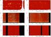 |
Fig. 6. Comparison of Ko Hα maps for Carrington rotations 854 (23 July to 18 August 1917, left) and 1497 (29 July to 25 August 1965, right, see also the top row of Figs. 1, 3 and 4 and the right column of Fig. 7) processed in this study (top row) by Chatterjee et al. (2017, middle row) and by Lin et al. (2020, bottom row). |
In Fig. 7 we compare our Carrington maps produced with MD data to drawings from the same site produced manually by the observers (Laurenceau et al. 2015)4 where they mark the locations of filaments and plage. We find a general agreement between the filaments seen in our calibrated images and the drawings. However, we also note some disagreements, such as for rotation 1497 over longitudes 120–200° in the southern hemisphere, for which the appearance of filaments is quite different in the two maps. We also note that low-contrast and fragmented filaments in our produced maps, such as the one for rotation 1497 over longitudes 40–180° in the northern hemisphere, are reported as connected in the Meudon drawings.
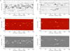 |
Fig. 7. Comparison of MD Hα maps for Carrington rotations 1427 (7 May to 2 June 1960, left, see also the middle column of Fig. 5) and 1497 (29 July to 25 August 1965, right, see also the top row of Figs. 1, 3 and 4 and right column of Fig. 6) produced manually by observations at Meudon (top row) and processed in this study (middle row). The bottom row shows the map obtained by overlapping the two corresponding maps shown in the upper two rows. To help visibility, this map is shown in greyscale, and the filaments from the manual processing (top panel) are shown in light grey instead of black. |
We emphasise that any analysis of a single database is affected by the limited time coverage, as it may not capture the dynamic nature of filaments. This limitation can be alleviated by applying accurate and homogeneous processing to data from different archives, however, using as many data from different sources as possible, as was done in our study.
3.2. Filament areas
Here we discuss and compare the resulting filament regions identified in the observations from the various Hα datasets. We identifed filaments in individual images and not on the Carrington maps (as was done in previous studies, e.g. Chatterjee et al. 2017), as this allows a more accurate identification of the features. We then transformed the produced masks into a Mercator representation of the identified filaments. Figure 4 shows example masks of the identified filaments from observations of various datasets. The identified features appear rather similar among data taken on the same day. However, we also note some differences that are mainly due to the bandwidth or central wavelength used for the observations, which seems to influence the appearance of the filaments. Some artefacts were unfortunately also still identified as filaments, for example the small and dark regions in the southern hemisphere of the Ar observations shown in Fig. 4.
Using the computed filament masks, we produced butterfly diagrams as time-versus-latitude maps. Figure 8 shows butterfly diagrams of the filament fractional area in bins of latitude of 1° from all individual archives. The poleward migration of filaments is clearly seen. This is evident for archives with good temporal coverage (e.g. BB, Bo, Ka, Ko, MD, Mi, and SP), and it is less clear for archives with only a few observations (e.g. Ar, Kh, La, and UP). We also note differences in the produced butterfly diagrams that are largely due to the differences of the archives. We do not note, however, any clear change in the butterfly diagram due to the transition from plates to CCD, as in the cases of Co, MD, Ka, or Mi. An interesting case is that of PM, for which the data appear to be taken off-band since late 2013. The resulting butterfly diagram, shown also in Fig. 9 enlarged compared to Fig. 8, displays the transition very clearly, with very few to no filaments registered after 2013. This suggests that PM data after 2013 unfortunately are not a good source of information on filaments.
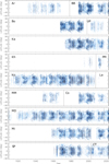 |
Fig. 8. Filament butterfly diagrams constructed from the observations of all Hα archives. The diagrams show daily mean areas within latitudinal strips of 1° as fractions of the area of the entire solar disc. White means no observed filaments, and blue denotes the filament fractional areas that become darker with growing areas up to the saturation level of 2×10⁻⁴. A vertical black line marks the separation of archives when more than one archive is included in a panel, except for MD, where it marks the instrument upgrade over 2017. |
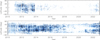 |
Fig. 9. Filament butterfly diagrams constructed from the observations of PM (top) Hα archive compared to those from Mi (bottom). The diagrams show daily mean filament areas within latitudinal strips of 1° as fractions of the area of the entire solar disc. White means no observed filaments, and blue denotes the filament fractional areas that become darker with growing areas up to the saturation level of 2 × 10⁻⁴. |
Figure 10 shows the disc-integrated filament areas from five long-running historical datasets analysed in this study (Bo, Ar, Ka, Ko, and MD) along with the international sunspot number (ISN hereafter; Clette et al. 2023) series. The figure also includes the asymmetric 1σ intervals (determined separately for the values that are higher and lower than the annual mean values) as a measure of uncertainty and spread of values within a year. We note a different behaviour among the various archives. For instance, the disc-integrated filament areas increase with time in the Ko series, which parallels the behaviour of plage areas in Ko Ca II K data (Chatzistergos et al. 2019b,d), suggesting that the increasing trend of quantities shown by both series is at least partly affected by the varying quality of the Ko data (see also Appendix A). In general, we do not see that the disc-integrated filament areas show the same cycle ranking as ISN. Particularly cycle 19, which is the strongest cycle in ISN, is comparatively normal in filament areas in all archives we analysed in this study. We note that over the covered period, ISN and the various group sunspot number series agree (e.g. Svalgaard & Schatten 2016; Chatzistergos et al. 2017; Usoskin et al. 2021), and thus our discussion is not affected by considering a different sunspot series.
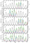 |
Fig. 10. Filament fractional areas derived from the Bo (a), Ar (b), Ka (c), Ko (d), and MD (e) Hα archives. We show annual median values of the disc-integrated areas (green) as well as polar filament fractional areas (multiplied by 10) for latitudes −90° to −50° (red) and 50° to 90° (blue). The shaded green surface denotes the asymmetric 1σ interval of the disc-integrated areas. We also show in black the ISN series. Its values are given on the right y-axis. The numbers within the panels denote the conventional solar cycle numbering. |
In Fig. 10 we also show the areas of polar filament regions (multiplied by 10), defined as those at latitudes greater than |50|°. Polar filaments appear at the beginning of a solar cycle, and when the cycle reaches its maximum, their areas decrease almost to zero. However, we note that the appearance of polar filaments for cycle 20 started earlier than in other cycles. The different series generally but not always agree in the hemispheric asymmetry of polar filaments. A notable exception is cycle 22, where MD and Ko show no asymmetry, while Bo and Ka show higher areas of polar filaments in the northern hemisphere.
Figure 11 shows annual mean disc-integrated filament areas from all analysed archives. There are significant differences between the various series, but we recall that this is expected due to the different sampling in the different series and the observational differences of the various series (Chatzistergos et al. 2020b, 2022). We recall that the appearance of filaments changes depending on the employed bandwidth (as well as filter transmission shape) of the observations, the central wavelength, but also the spatial resolution and thus the ability to resolve small filaments. Furthermore, because filaments are rather dynamic features, significant changes might occur even within relatively short time differences between the observations. In order to confirm the consistency of the series, we linearly scaled the filament areas from all series to match those by MD. The resulting filament areas are shown in the lower panel of Fig. 11. They display an improved agreement after the scaling. However, some discrepancies persist, such as in cycle 18, over which the filament areas from Ko are significantly lower than those from the other series.
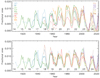 |
Fig. 11. Filament fractional areas from all analysed archives. The top panel shows the original areas, and the lower panel shows the areas after they were linearly scaled to match those from MD. The numbers within the panels denote the conventional solar cycle numbering. |
Finally, we combined results from all datasets together to produce an average series of filament fractional areas, which is shown in Fig. 12. To do this, we excluded PM data after 2014 as well as Ko data after 1998. Figure 12 also shows the evolution of the disc-integrated filament fractional areas in comparison to ISN. We find the filament fractional areas to be higher in cycles 20–23 than in earlier cycles or cycle 24, in contrast to ISN. We note that Tlatov et al. (2016) reported a similar increase in the number of filaments in MD data in cycles 22 and 23 compared to earlier cycles. Figure 12 also includes the average series of filament fractional areas over two latitudinal bands of [−90° to −50°] and [50° to 90°]. We find the rise of most cycles to largely coincide with that in ISN. Notable exceptions are cycle 20, over which we note an earlier increase only in the northern hemisphere, and cycle 23, for which the filament areas increase before ISN. Our results also suggest very few polar filaments in cycles 15 and 16.
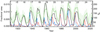 |
Fig. 12. Fractional filament areas derived from the composite filament area series. We show annual median values of the disc-integrated areas (green) as well as polar filament fractional areas (multiplied by 10) for latitudes −90° to −50° (red) and 50° to 90° (blue). The shaded green surface denotes the asymmetric 1σ interval of the disc-integrated areas. We also show in black the ISN series. Its values are given on the right y-axis. The numbers within the panels denote the conventional solar cycle numbering. |
Figure 13 shows a composite butterfly diagram derived by combining the filament areas from all data analysed in this study after linearly scaling them to match those from MD. We averaged all existing values on days for which multiple archives have data. This is to our knowledge the most complete filament butterfly diagram to date. The composite diagram highlights the characteristics of filament evolution, and in particular, their poleward migration.
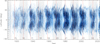 |
Fig. 13. Composite filament butterfly diagram constructed from the observations of all Hα archives, except for PM after 2014 and Ko after 1998 (see Sects. 2.1 and 3). The diagram shows daily mean areas within latitudinal strips of 1° as fractions of the area of the entire solar disc. White means no observed filaments, and blue denotes the filament fractional areas that become darker with growing areas up to the saturation level of 3 × 10⁻⁴. Even-numbered cycles are shaded in grey. The numbers in the lower part of the panel denote the conventional solar cycle numbering, and the date of the maximum of each cycle as defined by Sunspot Index and Long-term Solar Observations (SILSO, https://www.sidc.be/SILSO/cyclesminmax) is marked with a vertical red line. |
4. Summary and conclusions
Regular Hα photographic observations of the solar disc date back to 1909. Several series of these observations have recently been made available in digital form.
Observations in the Hα line are a great resource of information about the chromosphere, and particularly, about filament regions. These fascinating solar features trace the magnetic polarity-inversion lines, and thus, an analysis of the filament characteristics is important for understanding solar magnetism. Filament data have the potential of aiding reconstructions of past solar magnetograms based on Ca II K observations (Chatzistergos et al. 2019a), where Hα observations can provide information about the polarity of regions. Mordvinov et al. (2020) developed a method for the reconstruction of the solar magnetic field using the synoptic observations of the solar emission in the Ca II K and Hα lines from Ko. Based on these reconstructed magnetic maps, they studied the evolution of the magnetic field in cycles 15–19. Despite numerous previous works with such data, a consistent and accurate processing of the various archives, including in particular the photometric calibration of historical photographic archives, has been lacking.
We analysed the most prominent historical archives currently available in digital form along with some modern CCD-based ones. The historical archives include those from Kodaikanal, Meudon, Kanzelhöhe, and Sacramento Peak, which have been analysed before, but also those from Arcetri, Boulder, Coimbra, McMath-Hulbert, and Mitaka, which to our knowledge have not previously been used to study filaments in an automatic way. We recall that 9 of the 15 analysed series were not explored so far, thus assessing their characteristics also allows us to establish their potential for long-term studies of solar magnetism. We showed that our processing better accounted for most of the artefacts affecting the images than previous analyses of these data allowed. We produced Carrington maps from the calibrated Hα observations. We also developed an automatic approach to identify filaments in the images from the various archives. We produced butterfly (time/latitude) diagrams from each archive separately, as well as a composite diagram by considering all observations together, where we averaged all available observations on days when data from more than one observatory exist. We note that the observational characteristics of the various archives differ significantly. This means that different heights of the solar atmosphere are sampled, and it thus affects the characteristics of the filament regions. A more comprehensive study of the characteristics of the identified filaments from the different archives is very important to help us understand the differences between the various archives further.
It is worth noting that some of the archives have nearly cotemporal observations in the Ca II K line. Analysing these series can therefore also provide insights into Ca II K data. We studied the image characteristics of the various series and found common aspects with those previously reported for their Ca II K counterparts. In particular, we find both Ca II K and Hα observations from Ko to show a steady deterioration, or that both SP Ca II K and Hα observations exhibit a high disc ellipticity over the first ∼15 years. Finally, more historical Hα archives exist that are not available in digital format at the moment, such as those from Baikal (Golovko et al. 2002), Crimea, Ebro (Curto et al. 2016), Hamburg, Schauinsland, Wendelstein (Wöhl 2005), and Kislovodsk (Tlatov et al. 2016). It would be very beneficial if these archives could be digitised, along with the remaining data from Kharkiv and Larissa, in order to complement the available information of Hα data, and thus raise their reliability and value.
The Carrington maps are available at https://kso.iiap.res.in/new/H_alpha
Available at https://sun.bao.ac.cn/hsos_data/GHA/synMap/KODA/
Available at https://bass2000.obspm.fr/lastsynmap.php
Acknowledgments
The authors thank the observers at the Arcetri, Big Bear, Boulder, Catania, Coimbra, Kanzelhöhe, Kharkiv, Kodaikanal, Larissa, McMath-Hulbert, Meudon, Mitaka, Pic du Midi, Sacramento Peak, and Upice sites. We thank Hardi Peter and Sami K. Solanki for the fruitful discussions. We also thank Isabelle Buale for all her efforts to digitise the Meudon archive. We thank the anonymous referee for the constructive comments that helped improve this paper. We acknowledge Paris Observatory for the use of spectroheliograms. S.P. Spectroheliograms were acquired at Evans facility at Sac Peak operated by NSO/AURA/NSF, while the images were scanned by Dr. A. Tlatov (Russia). This work utilizes data from the National Solar Observatory Integrated Synoptic Program, which is operated by the Association of Universities for Research in Astronomy, under a cooperative agreement with the National Science Foundation and with additional financial support from the National Oceanic and Atmospheric Administration, the National Aeronautics and Space Administration, and the United States Air Force. The GONG network of instruments is hosted by the Big Bear Solar Observatory, High Altitude Observatory, Learmonth Solar Observatory, Udaipur Solar Observatory, Instituto de Astrofísica de Canarias, and Cerro Tololo Interamerican Observatory. Hα data were provided by the Kanzelhöhe Observatory, University of Graz, Austria. Larissa observatory acknowledges funding from the Municipality of Larissa, Thessaly, Greece. This work was supported by grants PRIN-INAF-2014 and PRIN/MIUR 2012P2HRCR “Il Sole attivo”, COST Action ES1005 “TOSCA”, FP7 SOLID. This research has received funding from the European Union’s Horizon 2020 research and innovation program under grant agreement No. 824135 (SOLARNET). T.C. thanks ISSI for supporting the International Team 474 “What Determines The Dynamo Effectivity Of Solar Active Regions?”. T.B., R.G., and N.P., acknowledge financial support by Fundação para a Ciência e a Tecnologia (FCT) through the research grants UIDB/04434/2020 and UIDP/04434/2020. This research has made use of NASA’s Astrophysics Data System (ADS; https://ui.adsabs.harvard.edu/) Bibliographic Services.
References
- Asvestari, E., Pomoell, J., Kilpua, E., et al. 2021, A&A, 652, A27 [NASA ADS] [CrossRef] [EDP Sciences] [Google Scholar]
- Babcock, H. W., & Babcock, H. D. 1955, ApJ, 121, 349 [Google Scholar]
- Belkina, I. L., Beletskij, S. A., Gretskij, A. M., & Marchenko, G. P. 1996, Kinemat. Phys. Celest. Bodies, 12, 55 [NASA ADS] [Google Scholar]
- Benkhalil, A., Zharkova, V. V., Ipson, S. S., & Zharkov, S. I. 2005, I. J. Comput. Appl., 12, 21 [Google Scholar]
- Bocchino, G. 1933, Mem. Soc. Astron. It., 6, 479 [NASA ADS] [Google Scholar]
- Bovelet, B., & Wiehr, E. 2001, Sol. Phys., 201, 13 [NASA ADS] [CrossRef] [Google Scholar]
- Boyd, R. W. 1978, J. Opt. Soc. Am., 68, 877 [NASA ADS] [CrossRef] [Google Scholar]
- Calabretta, M. R., & Greisen, E. W. 2002, A&A, 395, 1077 [NASA ADS] [CrossRef] [EDP Sciences] [Google Scholar]
- Carlsson, M., De Pontieu, B., & Hansteen, V. H. 2019, ARA&A, 57, 189 [Google Scholar]
- Carrasco, V. M. S., & Vaquero, J. M. 2022, ApJS, 262, 44 [CrossRef] [Google Scholar]
- Carrasco, V. M. S., Nogales, J. M., Vaquero, J. M., Chatzistergos, T., & Ermolli, I. 2021, J. Space Weather Space Clim., 11, 51 [NASA ADS] [CrossRef] [EDP Sciences] [Google Scholar]
- Chatterjee, S., Hegde, M., Banerjee, D., & Ravindra, B. 2017, ApJ, 849, 44 [NASA ADS] [CrossRef] [Google Scholar]
- Chatterjee, S., Hegde, M., Banerjee, D., Ravindra, B., & McIntosh, S. W. 2020, Earth Space Sci., 7, e2019EA000666 [CrossRef] [Google Scholar]
- Chatzistergos, T. 2017, PhD Thesis, University of Göttingen, Germany [Google Scholar]
- Chatzistergos, T., Ermolli, I., Solanki, S. K., & Krivova, N. A. 2016, in Coimbra Solar Physics Meeting: Ground-based Solar Observations in the Space Instrumentation Era, eds. I. Dorotovic, C. E. Fischer, & M. Temmer, ASP Conf. Ser., 504, 227 [NASA ADS] [Google Scholar]
- Chatzistergos, T., Usoskin, I. G., Kovaltsov, G. A., Krivova, N. A., & Solanki, S. K. 2017, A&A, 602, A69 [NASA ADS] [CrossRef] [EDP Sciences] [Google Scholar]
- Chatzistergos, T., Ermolli, I., Solanki, S. K., & Krivova, N. A. 2018a, A&A, 609, A92 [NASA ADS] [CrossRef] [EDP Sciences] [Google Scholar]
- Chatzistergos, T., Ermolli, I., Krivova, N. A., & Solanki, S. K. 2018b, in Long-term Datasets for the Understanding of Solar and Stellar Magnetic Cycles, eds. D. Banerjee, J. Jiang, K. Kusano, & S. Solanki (Cambridge, UK: Cambridge University Press), IAU Symp., 340, 125 [NASA ADS] [Google Scholar]
- Chatzistergos, T., Ermolli, I., Solanki, S. K., et al. 2019a, A&A, 626, A114 [NASA ADS] [CrossRef] [EDP Sciences] [Google Scholar]
- Chatzistergos, T., Ermolli, I., Krivova, N. A., & Solanki, S. K. 2019b, A&A, 625, A69 [NASA ADS] [CrossRef] [EDP Sciences] [Google Scholar]
- Chatzistergos, T., Ermolli, I., Falco, M., et al. 2019c, Il Nuovo Cimento, 42C, 5 [Google Scholar]
- Chatzistergos, T., Ermolli, I., Solanki, S. K., et al. 2019d, Sol. Phys., 294, 145 [NASA ADS] [CrossRef] [Google Scholar]
- Chatzistergos, T., Ermolli, I., Krivova, N. A., & Solanki, S. K. 2020a, J. Phys.: Conf. Ser., 1548, 012007 [NASA ADS] [CrossRef] [Google Scholar]
- Chatzistergos, T., Ermolli, I., Krivova, N. A., et al. 2020b, A&A, 639, A88 [NASA ADS] [CrossRef] [EDP Sciences] [Google Scholar]
- Chatzistergos, T., Ermolli, I., Giorgi, F., Krivova, N. A., & Puiu, C. C. 2020c, J. Space Weather Space Clim., 10, 45 [NASA ADS] [CrossRef] [EDP Sciences] [Google Scholar]
- Chatzistergos, T., Krivova, N. A., Ermolli, I., et al. 2021, A&A, 656, A104 [NASA ADS] [CrossRef] [EDP Sciences] [Google Scholar]
- Chatzistergos, T., Krivova, N. A., & Ermolli, I. 2022, Front. Astron. Space Sci., 9, 1038949 [CrossRef] [Google Scholar]
- Chatzistergos, T., Krivova, N. A., & Yeo, K. L. 2023, JASTP, 252, 106150 [NASA ADS] [Google Scholar]
- Clette, F., Lefèvre, L., Chatzistergos, T., et al. 2023, Sol. Phys., 298, 44 [NASA ADS] [CrossRef] [Google Scholar]
- Coffey, H. E., & Hanchett, C. D. 1998, in IAU Colloq. 167: New Perspectives on Solar Prominences, eds. D. Webb, D. Rust, & B. Schmieder, ASP Conf. Ser., 150, 488 [NASA ADS] [Google Scholar]
- Corbard, T., Ikhlef, R., Morand, F., Meftah, M., & Renaud, C. 2019, MNRAS, 483, 3865 [CrossRef] [Google Scholar]
- Curto, J. J., Solé, J. G., Genescà, M., Blanca, M. J., & Vaquero, J. M. 2016, Sol. Phys., 291, 2587 [NASA ADS] [CrossRef] [Google Scholar]
- Denker, C., Johannesson, A., Marquette, W., et al. 1999, Sol. Phys., 184, 87 [NASA ADS] [CrossRef] [Google Scholar]
- De Pontieu, B., Hansteen, V. H., Rouppe van der Voort, L., van Noort, M., & Carlsson, M. 2007, ApJ, 655, 624 [Google Scholar]
- Diercke, A., & Denker, C. 2019, Sol. Phys., 294, 152 [NASA ADS] [CrossRef] [Google Scholar]
- Diercke, A., Kuckein, C., Cauley, P. W., et al. 2022, A&A, 661, A107 [NASA ADS] [CrossRef] [EDP Sciences] [Google Scholar]
- Ermolli, I., & Ferrucci, M. 2021, in Angelo Secchi and Nineteenth Century Science: The Multidisciplinary Contributions of a Pioneer and Innovator, eds. I. Chinnici, & G. Consolmagno (Cham: Springer International Publishing), Hist. Cult. Astron., 123 [Google Scholar]
- Ermolli, I., Solanki, S. K., Tlatov, A. G., et al. 2009a, ApJ, 698, 1000 [NASA ADS] [CrossRef] [Google Scholar]
- Ermolli, I., Marchei, E., Centrone, M., et al. 2009b, A&A, 499, 627 [NASA ADS] [CrossRef] [EDP Sciences] [Google Scholar]
- Ermolli, I., Chatzistergos, T., Krivova, N. A., & Solanki, S. K. 2018, in Long-term Datasets for the Understanding of Solar and Stellar Magnetic Cycles, eds. D. Banerjee, J. Jiang, K. Kusano, & S. Solanki (Cambridge, UK: Cambridge University Press), IAU Symp., 340, 115 [NASA ADS] [Google Scholar]
- Ermolli, I., Giorgi, F., & Chatzistergos, T. 2022, Front. Astron. Space Sci., 9, 1042740 [CrossRef] [Google Scholar]
- Ermolli, I., Chatzistergos, T., Giorgi, F., et al. 2023, ApJS, in press, https://doi.org/10.3847/1538-4365/ad0886 [Google Scholar]
- Freeland, S., & Handy, B. 1998, Sol. Phys., 182, 497 [NASA ADS] [CrossRef] [Google Scholar]
- Fuller, N., Aboudarham, J., & Bentley, R. D. 2005, Sol. Phys., 227, 61 [NASA ADS] [CrossRef] [Google Scholar]
- Golovko, A. A., Golubeva, E. M., Grechnev, V. V., et al. 2002, Solar Variability: From Core to Outer Frontiers (ESA Publications Division), 506, 929 [NASA ADS] [Google Scholar]
- Hale, G. E. 1904, Popular Science Monthly (Science Press), 65, 5 [Google Scholar]
- Hanaoka, Y., Sakurai, T., Otsuji, K., Suzuki, I., & Morita, S. 2020, J. Space Weather Space Clim., 10, 41 [NASA ADS] [CrossRef] [EDP Sciences] [Google Scholar]
- Hansen, R., & Hansen, S. 1975, Sol. Phys., 44, 225 [NASA ADS] [CrossRef] [Google Scholar]
- Hao, Q., Fang, C., & Chen, P. F. 2013, Sol. Phys., 286, 385 [NASA ADS] [CrossRef] [Google Scholar]
- Hao, Q., Fang, C., Cao, W., & Chen, P. F. 2015, ApJS, 221, 33 [NASA ADS] [CrossRef] [Google Scholar]
- Janssen, M. 1869, Proc. R. Soc. London, 17, 276 [NASA ADS] [CrossRef] [Google Scholar]
- Jha, B. K. 2022, https://zenodo.org/records/7651499 [Google Scholar]
- Klimeš, J., Bělik, M., Klimeš, J., & Marková, E. 1999, in 8th SOHO Workshop: Plasma Dynamics and Diagnostics in the Solar Transition Region and Corona, eds. J. C. Vial, & B. Kaldeich-Schü, ESA Spec. Publ., 446, 375 [Google Scholar]
- Koechlin, L., Dettwiller, L., Audejean, M., Valais, M., & Ariste, A. L. 2019, A&A, 631, A55 [NASA ADS] [CrossRef] [EDP Sciences] [Google Scholar]
- Laurenceau, A., Aboudarham, J., & Renié, C. 2015, in Library and Information Services in Astronomy VII: Open Science at the Frontiers of Librarianship, eds. A. Holl, S. Lesteven, D. Dietrich, & A. Gasperini, ASP Conf. Ser., 492, 155 [NASA ADS] [Google Scholar]
- Li, K. J., Li, Q. X., Gao, P. X., et al. 2007, JApA, 28, 147 [NASA ADS] [Google Scholar]
- Lin, G., Zhu, G., Yang, X., et al. 2020, ApJS, 249, 11 [NASA ADS] [CrossRef] [Google Scholar]
- Lockyer, J. N., & Frankland, P. F. 1869, Proc. R. Soc. London, 17, 350 [NASA ADS] [CrossRef] [Google Scholar]
- Lourenço, A., Carvalho, S., Barata, T., et al. 2019, Open Astron., 28, 165 [CrossRef] [Google Scholar]
- Lourenço, A., Gafeira, R., Bonifácio, V., et al. 2021, Sol. Phys., 296, 155 [CrossRef] [Google Scholar]
- Makarov, V. I., & Sivaraman, K. R. 1983, Sol. Phys., 85, 227 [NASA ADS] [CrossRef] [Google Scholar]
- Makarov, V. I., Stoianova, M. N., & Sivaraman, K. R. 1982, JApA, 3, 379 [NASA ADS] [Google Scholar]
- Makarov, V. I., Fatianov, M. P., & Sivaraman, K. R. 1983, Sol. Phys., 85, 215 [NASA ADS] [CrossRef] [Google Scholar]
- Malherbe, J. M. 2023, J. Hist. Astron., 54, 274 [NASA ADS] [CrossRef] [Google Scholar]
- Malherbe, J.-M., & Dalmasse, K. 2019, Sol. Phys., 294, 52 [NASA ADS] [CrossRef] [Google Scholar]
- Martin, S. F. 1998, Sol. Phys., 182, 107 [Google Scholar]
- Mazumder, R., Chatterjee, S., Nandy, D., & Banerjee, D. 2021, ApJ, 919, 125 [NASA ADS] [CrossRef] [Google Scholar]
- McIntosh, P. S. 1972, Rev. Geophys. Space Phys., 10, 837 [CrossRef] [Google Scholar]
- Mohler, O. C., & Dodson, H. W. 1968, Sol. Phys., 5, 417 [NASA ADS] [CrossRef] [Google Scholar]
- Mordvinov, A. V., Karak, B. B., Banerjee, D., et al. 2020, ApJ, 902, L15 [NASA ADS] [CrossRef] [Google Scholar]
- Mouradian, Z. 1998, Synop. Sol. Phys., 140, 197 [NASA ADS] [Google Scholar]
- Murabito, M., Ermolli, I., Chatzistergos, T., et al. 2023, ApJ, 947, 18 [NASA ADS] [CrossRef] [Google Scholar]
- Parenti, S. 2014, Liv. Rev. Sol. Phys., 11, 1 [Google Scholar]
- Pereira, T. M. D., De Pontieu, B., & Carlsson, M. 2012, ApJ, 759, 18 [Google Scholar]
- Pötzi, W. 2008, Cent. Eur. Astrophys. Bull., 32, 9 [Google Scholar]
- Pötzi, W., Veronig, A., Jarolim, R., et al. 2021, Sol. Phys., 296, 164 [CrossRef] [Google Scholar]
- Righini, G., & Godoli, G. 1950, Mem. Soc. Astron. It., 21, 333 [NASA ADS] [Google Scholar]
- Rimmele, T. R., & Marino, J. 2011, Liv. Rev. Sol. Phys., 8, 2 [Google Scholar]
- Romano, P., Guglielmino, S. L., Costa, P., et al. 2022, Sol. Phys., 297, 7 [NASA ADS] [CrossRef] [Google Scholar]
- Rouppe van der Voort, L., Leenaarts, J., de Pontieu, B., Carlsson, M., & Vissers, G. 2009, ApJ, 705, 272 [Google Scholar]
- Secchi, A. 1871, Sulla distribuzione delle protuberanze intorno AL disco solare (Roma: Tipografia delle scienze matematiche e fisiche) [Google Scholar]
- Shih, F. Y., & Kowalski, A. J. 2003, Sol. Phys., 218, 99 [NASA ADS] [CrossRef] [Google Scholar]
- Suo, L. 2020, Adv. Space Res., 65, 1054 [NASA ADS] [CrossRef] [Google Scholar]
- Svalgaard, L., & Schatten, K. H. 2016, Sol. Phys., 291, 2653 [NASA ADS] [CrossRef] [Google Scholar]
- Tacchini, P. 1872, Mem. Soc. Spectrosc. It., 1, 123 [NASA ADS] [Google Scholar]
- Tlatov, A. G., Pevtsov, A. A., & Singh, J. 2009, Sol. Phys., 255, 239 [NASA ADS] [CrossRef] [Google Scholar]
- Tlatov, A. G., Kuzanyan, K. M., & Vasil’yeva, V. V. 2016, Sol. Phys., 291, 1115 [NASA ADS] [CrossRef] [Google Scholar]
- Tsiropoula, G., Alissandrakis, C. E., & Schmieder, B. 1994, A&A, 290, 285 [NASA ADS] [Google Scholar]
- Usoskin, I., Kovaltsov, G., & Kiviaho, W. 2021, Sol. Phys., 296, 13 [Google Scholar]
- Vernazza, J. E., Avrett, E. H., & Loeser, R. 1981, ApJS, 45, 635 [Google Scholar]
- Wallace, R. J. 1907, ApJ, 26, 299 [NASA ADS] [CrossRef] [Google Scholar]
- Wan, M., & Li, K. 2022, Sol. Phys., 297, 126 [NASA ADS] [CrossRef] [Google Scholar]
- Wöhl, H. 2005, Hvar Obs. Bull., 29, 319 [Google Scholar]
- Wu, S. T., Dryer, M., McIntosh, P. S., & Reichmann, E. 1975, Sol. Phys., 44, 117 [NASA ADS] [CrossRef] [Google Scholar]
- Yuan, Y., Shih, F. Y., Jing, J., Wang, H., & Chae, J. 2011, Sol. Phys., 272, 101 [NASA ADS] [CrossRef] [Google Scholar]
- Zharkova, V. V., & Schetinin, V. 2005, Sol. Phys., 228, 137 [NASA ADS] [CrossRef] [Google Scholar]
- Zou, P., Li, Q.-X., & Wu, N. 2014, MNRAS, 437, 38 [NASA ADS] [CrossRef] [Google Scholar]
Appendix A: Archive characteristics
Here we discuss some characteristics of the digital images from the various archives we analysed. Following Ermolli et al. (2009a) and Chatzistergos et al. (2019d), we studied the solar disc eccentricity, the spatial resolution, the large-scale inhomogeneities, and the mean standard error between the measured QS CLV to the reference QS CLV (taken to be the one from CT data). Table A.1 and Fig. A.1 show the results for the characteristics of the various archives used in this study. Findings from this study helped us to optimise details in steps of our image processing and provided new information about the analysed archives. We recall that 9 of the 15 analysed series were not explored so far, thus assessing their characteristics also allows us to establish their potential for long-term studies of solar processes.
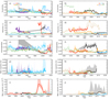 |
Fig. A.1. Temporal evolution of key characteristics of the raw Hα data. Panels a) and b): Eccentricity of the recorded solar disc. Panels c) and d): Spatial resolution. Panels e) and f): Large-scale inhomogeneities. Panels g)–j): Mean-squared error of the fit to the curve relating the measured QS CLV from the various archives to the reference QS CLV obtained from CT data. The latter is shown separately for the photographic data (panels g and h) and the CCD-based ones (panels i and j). The legend in the top panels gives the colour association of the different archives. We show annual median values, along with their asymmetric 1σ intervals (shaded surfaces; see Appendix A for more details). |
Determined characteristics of the Hα archives.
We first compared the solar disc eccentricity, defined as  , where Rmin and Rmax are the semi-minor and -major axes as measured with a fit of an ellipse to the edge of the solar disc, which was identified with Sobel filtering (for more details, see Appendix B of Chatzistergos et al. 2019b, and Chatzistergos et al. 2020a). We note that there are various reasons that can cause the recorded solar disc to show a roughly elliptical shape, including atmospheric diffraction (Corbard et al. 2019), potential tilts between the optical axis and the camera, and issues during the digitisation of the plates. However, the most common reason for spectroheliograms to exhibit elliptical (and sometimes rather distorted) solar discs is an uneven motion of the instrument, which causes some rasters to be stretched unevenly compared to others in the recorded image. We find all archives to have rather similar eccentricities, with mean values within 0.06 and 0.2. The CCD-based data have slightly lower values. We note, however, that there are periods with increased disc ellipticity for some archives, for instance SP data before 1975, BB data before 1996, Co data before 2008, or Ko data over 1972–1976 and after 1998. The results for SP are consistent with those for the SP Ca II K data for the increased ellipticity before 1975 (Chatzistergos et al. 2020a). The decrease in ellipticity in the Co data coincides with the introduction of the CCD camera. We note that a similar decrease is seen in MD data over 2002 when the CCD camera was introduced, but the change is smaller than for Co data. For Ko data after 1998, we note that the values for the ellipticity (and most metrics in the following) are not reliable because almost all of these data miss large parts of the disc (see Sect. 2.1).
We compared the spatial resolution of the observations by finding the frequency for which the 98% of the power spectral density of the solar disc was taken into account. Following Chatzistergos et al. (2019d), we performed the computation within 64×64 pixel2 sub-arrays of QS regions. This was repeated 100 times by randomly selecting a different QS region across the inner R/3 of the solar disc. The mean value of the 100 computations was adopted as the mean spatial resolution of the images. Most archives analysed in this study exhibit a rather stable spatial resolution with time. The spatial resolution for the Ko data increases almost constantly with time, suggesting worsening conditions with time. This is consistent with the results for the Ko Ca II K data (Chatzistergos et al. 2019d). The spatial resolution of the MD observations is rather stable with time. We note a decrease in spatial resolution with time for Ar, Ka, and BB data, while Mi data increase after 1990 and decrease after 2011. For BB, Ka, and Mi data, this is mostly due to changes in the pixel scale of the observations. The decrease in spatial resolution of Ar data is partly due to saturated regions in some images in the early periods. This is consistent with the Ar Ca II K data as well (Chatzistergos et al. 2019b).
Then we evaluated the large-scale inhomogeneities that affect the observations. Following Chatzistergos et al. (2019d), we defined a measure of the inhomogeneities as the relative difference of the computed background of the images to the radially symmetric QS CLV. Most archives analysed in this study show a rather stable level of inhomogeneities with time. We find a decrease in the inhomogeneities with time for the SP and MD archives, while there is an abrupt decrease for the Co data over 2008 that coincides with the installation of the CCD camera. In contrast to this, there is a considerable increase in the BB data after 2010. Many BB images in that period show artefacts that were probably introduced during the calibration of the CCD, rendering the centre of the disc darker than the regions close to the limb (see Fig. 1). We note, however, that these issues are treated accurately enough by our processing.
Finally, we computed the mean standard error of the fit between the measured QS CLV and a standard reference QS CLV. The reference QS CLV was the one we used for the photometric calibration of the historical data and was the mean QS CLV from selected CT data that were not affected by large-scale artefacts. We recall that CT observations were performed with a CCD camera. When computing the mean errors, we considered the photographic and CCD-based data separately because their results are not comparable. This is because the photographic data are given in values of density, while the CCD-based ones are already in intensity units. However, to make the results from the various CCD-based data comparable, we normalised the measured QS CLV pattern so that its maximum value was always one (this is needed because the bit depth of the images from different archives is different). Furthermore, the errors from all archives (both photographic and CCD-based ones) were divided by the degrees of freedom of the fit in each case to render them comparable to each other (this is needed because the solar disc dimensions in the images from different archives are different). The resulting mean errors for all photographic archives are relatively low in the range 0.0001–0.0020, while the standard deviation of the errors reaches values up to 0.005 when the Ko data after 1998 are ignored. We note that most archives contain periods for which the errors increase abruptly, but these tend to be for isolated years. For the Ko data, there is a slight increase of the error with time, similar to the one reported for the Ko Ca II K data (Chatzistergos et al. 2018a, 2019d), favouring the argument that this is due to worsening atmospheric conditions or instrumental wearing. However, the increase in the error for the Hα data is smaller than the one reported for the Ca II K data (Chatzistergos et al. 2019d). This might be due to the wavelength-dependent behaviour of seeing, which is less severe for longer wavelengths, in this case, Hα compared to Ca II K (Boyd 1978; Rimmele & Marino 2011), and thus supports the suggestion that the seeing conditions at Kodaikanal deteriorated with time. The errors for Ko data after 1998 reach a value of 0.12. The periods for which the errors for the Ko data exhibit abrupt changes do not match those from the Ko Ca II K data, which means that these particular ones are probably not due to instrumental issues. However, we note that this is not a robust test because it merely measures how different the QS CLV of the various data is to the reference set, while it might also be partly affected by severe large-scale inhomogeneities in the images. The results for the CCD-based data show even smaller variations (but we stress that the absolute values for the CCD-based and photographic data are not comparable). CT data were used to derive the reference QS CLV pattern, and they show rather low variations that are lower than 0.2×10⁻³. We note relatively low errors for archives with a bandwidth similar to that of CT, while the errors are slightly higher for MD and Co which have a narrower bandwidth. We also notice a sharp increase in the mean error for PM since 2014, which would be in line with the observation that PM data since that period were taken off-band. There is also a sharp increase in the mean error for BB data after 2011. This is due to artefacts of the images that caused the centre of the disc to be darker than the regions near the limb.
This analysis allowed us to identify archive inconsistencies, but also to verify some that were previously found in contemporaneous Ca II K data. Thus, this also has implications for studies with Ca II K data from the sites that have data contemporaneous to Hα, and importantly, for studies reconstructing previous solar magnetism (Chatzistergos et al. 2022) and solar irradiance (Chatzistergos et al. 2023).
All Tables
All Figures
|
Fig. 1. Examples of Hα observations from the various archives analysed in this study. The images within each row correspond to the same day, with the exception of the Kh image (taken on 26 May 2000). In particular, the dates of the observations are 4 August 1965 for Ar, Ko, MD, MM, and Mi; 14 January 1980 for Bo, Ka, MD, and SP; 2 September 2011 for BB, Ka, La, Mi, and UP; and 13 September 2013 for BB, CT, Co, Ka, and PM. The images are shown after the pre-processing to identify the disc and to resample them to account for the disc ellipticity (when applicable) and convert the historical data to density values. The images have been aligned to show the solar north pole at the top. |
| In the text | |
|
Fig. 2. Annual fractional coverage by the various Hα archives analysed in this study. The annual coverage by all the archives combined is shown as well. The annual coverage is colour-coded as shown by the colour bar plotted within the plot. The black boxes mark the years with complete daily coverage. |
| In the text | |
|
Fig. 3. Examples of photometrically calibrated and limb-darkening-compensated contrast images for the observations shown in Fig. 1. All images show contrast values in the range [ − 0.5, 0.5]. |
| In the text | |
|
Fig. 4. Examples of masks identifying filaments in the observations shown in Fig. 1. The circles mark the disc boundaries, and filaments are shown in black. The last column is overlaid on the masks from the various observations taken on the same day and shown in the corresponding row in blue, red, green, yellow, and purple. The observations in each row were taken on the same day, with the exception of Kh in the second row, which is why it is not overlaid in the last panel of the row. In the masks shown in the last column, we have compensated for the differential rotation to show all of them as they would have been at 12:00 UTC. |
| In the text | |
|
Fig. 5. Carrington maps constructed from the observations of nine Hα archives. Each column shows Carrington maps for the same rotations 1427 (7 May to 2 June 1960, left, see also the left column of Fig. 7), 1689 (30 November to 26 December 1979, middle), and 2141 (1 to 27 September 2013, right, see also the bottom row of Figs. 1–4). All maps show contrast values in the range [−0.5, 0.5]. |
| In the text | |
|
Fig. 6. Comparison of Ko Hα maps for Carrington rotations 854 (23 July to 18 August 1917, left) and 1497 (29 July to 25 August 1965, right, see also the top row of Figs. 1, 3 and 4 and the right column of Fig. 7) processed in this study (top row) by Chatterjee et al. (2017, middle row) and by Lin et al. (2020, bottom row). |
| In the text | |
|
Fig. 7. Comparison of MD Hα maps for Carrington rotations 1427 (7 May to 2 June 1960, left, see also the middle column of Fig. 5) and 1497 (29 July to 25 August 1965, right, see also the top row of Figs. 1, 3 and 4 and right column of Fig. 6) produced manually by observations at Meudon (top row) and processed in this study (middle row). The bottom row shows the map obtained by overlapping the two corresponding maps shown in the upper two rows. To help visibility, this map is shown in greyscale, and the filaments from the manual processing (top panel) are shown in light grey instead of black. |
| In the text | |
|
Fig. 8. Filament butterfly diagrams constructed from the observations of all Hα archives. The diagrams show daily mean areas within latitudinal strips of 1° as fractions of the area of the entire solar disc. White means no observed filaments, and blue denotes the filament fractional areas that become darker with growing areas up to the saturation level of 2×10⁻⁴. A vertical black line marks the separation of archives when more than one archive is included in a panel, except for MD, where it marks the instrument upgrade over 2017. |
| In the text | |
|
Fig. 9. Filament butterfly diagrams constructed from the observations of PM (top) Hα archive compared to those from Mi (bottom). The diagrams show daily mean filament areas within latitudinal strips of 1° as fractions of the area of the entire solar disc. White means no observed filaments, and blue denotes the filament fractional areas that become darker with growing areas up to the saturation level of 2 × 10⁻⁴. |
| In the text | |
|
Fig. 10. Filament fractional areas derived from the Bo (a), Ar (b), Ka (c), Ko (d), and MD (e) Hα archives. We show annual median values of the disc-integrated areas (green) as well as polar filament fractional areas (multiplied by 10) for latitudes −90° to −50° (red) and 50° to 90° (blue). The shaded green surface denotes the asymmetric 1σ interval of the disc-integrated areas. We also show in black the ISN series. Its values are given on the right y-axis. The numbers within the panels denote the conventional solar cycle numbering. |
| In the text | |
|
Fig. 11. Filament fractional areas from all analysed archives. The top panel shows the original areas, and the lower panel shows the areas after they were linearly scaled to match those from MD. The numbers within the panels denote the conventional solar cycle numbering. |
| In the text | |
|
Fig. 12. Fractional filament areas derived from the composite filament area series. We show annual median values of the disc-integrated areas (green) as well as polar filament fractional areas (multiplied by 10) for latitudes −90° to −50° (red) and 50° to 90° (blue). The shaded green surface denotes the asymmetric 1σ interval of the disc-integrated areas. We also show in black the ISN series. Its values are given on the right y-axis. The numbers within the panels denote the conventional solar cycle numbering. |
| In the text | |
|
Fig. 13. Composite filament butterfly diagram constructed from the observations of all Hα archives, except for PM after 2014 and Ko after 1998 (see Sects. 2.1 and 3). The diagram shows daily mean areas within latitudinal strips of 1° as fractions of the area of the entire solar disc. White means no observed filaments, and blue denotes the filament fractional areas that become darker with growing areas up to the saturation level of 3 × 10⁻⁴. Even-numbered cycles are shaded in grey. The numbers in the lower part of the panel denote the conventional solar cycle numbering, and the date of the maximum of each cycle as defined by Sunspot Index and Long-term Solar Observations (SILSO, https://www.sidc.be/SILSO/cyclesminmax) is marked with a vertical red line. |
| In the text | |
|
Fig. A.1. Temporal evolution of key characteristics of the raw Hα data. Panels a) and b): Eccentricity of the recorded solar disc. Panels c) and d): Spatial resolution. Panels e) and f): Large-scale inhomogeneities. Panels g)–j): Mean-squared error of the fit to the curve relating the measured QS CLV from the various archives to the reference QS CLV obtained from CT data. The latter is shown separately for the photographic data (panels g and h) and the CCD-based ones (panels i and j). The legend in the top panels gives the colour association of the different archives. We show annual median values, along with their asymmetric 1σ intervals (shaded surfaces; see Appendix A for more details). |
| In the text | |
Current usage metrics show cumulative count of Article Views (full-text article views including HTML views, PDF and ePub downloads, according to the available data) and Abstracts Views on Vision4Press platform.
Data correspond to usage on the plateform after 2015. The current usage metrics is available 48-96 hours after online publication and is updated daily on week days.
Initial download of the metrics may take a while.