| Issue |
A&A
Volume 679, November 2023
|
|
|---|---|---|
| Article Number | A90 | |
| Number of page(s) | 12 | |
| Section | Astronomical instrumentation | |
| DOI | https://doi.org/10.1051/0004-6361/202347128 | |
| Published online | 16 November 2023 | |
Star tracking for pointing determination of Imaging Atmospheric Cherenkov Telescopes
Application to the Large-Sized Telescope of the Cherenkov Telescope Array
1
Department of Physics, Tokai University,
4-1-1, Kita-Kaname, Hiratsuka,
Kanagawa
259-1292, Japan
2
Institute for Cosmic Ray Research, University of Tokyo,
5-1-5, Kashiwa-no-ha, Kashiwa,
Chiba
277-8582, Japan
3
Departament de Física Quàntica i Astrofísica, Institut de Ciències del Cosmos, Universitat de Barcelona, IEEC-UB,
Martí i Franquès 1,
08028,
Barcelona, Spain
4
Instituto de Astrofísica de Andalucía-CSIC,
Glorieta de la Astronomía s/n,
18008
Granada, Spain
5
Grupo de Electronica, Universidad Complutense de Madrid,
Av. Complutense s/n,
28040
Madrid, Spain
6
INAF - Osservatorio Astronomico di Roma,
Via di Frascati 33,
00040
Monteporzio Catone, Italy
7
INFN Sezione di Napoli,
Via Cintia, ed. G,
80126
Napoli, Italy
8
Max-Planck-Institut für Physik,
Föhringer Ring 6,
80805
München, Germany
9
INFN Sezione di Padova and Università degli Studi di Padova,
Via Marzolo 8,
35131
Padova, Italy
10
Institut de Fisica d’Altes Energies (IFAE), The Barcelona Institute of Science and Technology,
Campus UAB,
08193
Bellaterra (Barcelona), Spain
11
Univ. Savoie Mont Blanc, CNRS, Laboratoire d’Annecy de Physique des Particules - IN2P3,
74000
Annecy, France
12
Universität Hamburg, Institut für Experimentalphysik,
Luruper Chaussee 149,
22761
Hamburg, Germany
13
Graduate School of Science, University of Tokyo,
7-3-1 Hongo, Bunkyo-ku,
Tokyo
113-0033, Japan
14
EMFTEL department and IPARCOS, Universidad Complutense de Madrid,
Plaza de Ciencias, 1. Ciudad Universitaria,
28040
Madrid, Spain
15
INAF – Osservatorio di Astrofísica e Scienza dello spazio di Bologna,
Via Piero Gobetti 93/3,
40129
Bologna, Italy
16
Centro Brasileiro de Pesquisas Físicas,
Rua Xavier Sigaud 150,
RJ 22290-180,
Rio de Janeiro, Brazil
17
Instituto de Astrofísica de Canarias and Departamento de Astrofísica, Universidad de La Laguna,
C. Vía Láctea, s/n,
38205
La Laguna, Santa Cruz de Tenerife, Spain
18
CIEMAT,
Avda. Complutense 40,
28040
Madrid, Spain
19
Department of Physics, TU Dortmund University,
Otto-Hahn-Str. 4,
44227
Dortmund, Germany
20
INFN Sezione di Bari and Politecnico di Bari,
via Orabona 4,
70124
Bari, Italy
21
INAF – Osservatorio Astronomico di Brera,
Via Brera 28,
20121
Milano, Italy
22
INFN Sezione di Trieste and Università degli studi di Udine,
via delle scienze 206,
33100
Udine, Italy
23
University of Geneva - Département de physique nucléaire et corpusculaire,
24 Quai Ernest Ansernet,
1211
Genève 4, Switzerland
24
INFN Sezione di Catania,
Via S. Sofia 64,
95123
Catania, Italy
25
INAF - Istituto di Astrofísica e Planetologia Spaziali (IAPS),
Via del Fosso del Cavaliere 100,
00133
Roma, Italy
26
Aix-Marseille Univ, CNRS/IN2P3, CPPM,
Marseille, France
27
INFN Sezione di Torino,
Via P. Giuria 1,
10125
Torino, Italy
28
Palacky University Olomouc, Faculty of Science,
17. listopadu 1192/12,
771 46
Olomouc, Czech Republic
29
Port d’Informació Científica, Edifici D, Carrer de l’Albareda,
08193
Bellaterrra (Cerdanyola del Vallès), Spain
30
INFN Sezione di Bari and Università di Bari,
via Orabona 4,
70126
Bari, Italy
31
University of Rijeka, Department of Physics,
Radmile Matejcic 2,
51000
Rijeka, Croatia
32
Institute for Theoretical Physics and Astrophysics, Universität Würzburg,
Campus Hubland Nord, Emil-Fischer-Str. 31,
97074
Würzburg, Germany
33
Institut für Theoretische Physik, Lehrstuhl IV: Plasma-Astroteilchenphysik, Ruhr-Universität Bochum,
Universitätsstraße 150,
44801
Bochum, Germany
34
INFN Sezione di Roma La Sapienza,
P.le Aldo Moro 2,
00185
Rome, Italy
35
ILANCE, CNRS - University of Tokyo International Research Laboratory, University of Tokyo,
5-1-5 Kashiwa-no-Ha Kashiwa City,
Chiba
277-8582, Japan
36
Physics Program, Graduate School of Advanced Science and Engineering, Hiroshima University,
1-3-1 Kagamiyama, Higashi-Hiroshima City,
Hiroshima,
739-8526, Japan
37
INFN Sezione di Roma Tor Vergata,
Via della Ricerca Scientifica 1,
00133
Rome, Italy
38
Faculty of Physics and Applied Informatics, University of Lodz,
ul. Pomorska 149-153,
90-236
Lodz, Poland
39
University of Split, FESB,
R. Boškovića 32,
21000
Split, Croatia
40
Department of Physics, Yamagata University,
1-4-12 Kojirakawamachi,
Yamagata-shi,
990-8560, Japan
41
Josip Juraj Strossmayer University of Osijek, Department of Physics,
Trg Ljudevita Gaja 6,
31000
Osijek, Croatia
42
INFN Dipartimento di Scienze Fisiche e Chimiche - Università degli Studi dell’Aquila and Gran Sasso Science Institute,
Via Vetoio 1, Viale Crispi 7,
67100
L’Aquila, Italy
43
Kitashirakawa Oiwakecho, Sakyo Ward,
Kyoto,
606-8502, Japan
44
FZU - Institute of Physics of the Czech Academy of Sciences,
Na Slovance 1999/2,
182 21
Praha 8, Czech Republic
45
Astronomical Institute of the Czech Academy of Sciences,
Bocni II 1401,
14100
Prague, Czech Republic
46
Faculty of Science, Ibaraki University,
2 Chome-1-1 Bunkyo, Mito,
Ibaraki
310-0056, Japan
47
Faculty of Science and Engineering, Waseda University,
3 Chome-4-1 Okubo, Shinjuku City,
Tokyo
169-0072, Japan
48
Institute of Particle and Nuclear Studies, KEK (High Energy Accelerator Research Organization),
1-1 Oho,
Tsukuba,
305-0801, Japan
49
INFN Sezione di Trieste and Università degli Studi di Trieste,
Via Valerio 2 I,
34127
Trieste, Italy
50
INFN and Università degli Studi di Siena, Dipartimento di Scienze Fisiche, della Terra e dell’Ambiente (DSFTA),
Sezione di Fisica, Via Roma 56,
53100
Siena, Italy
51
Escuela Politécnica Superior de Jaén, Universidad de Jaén,
Campus Las Lagunillas s/n, Edif. A3,
23071
Jaén, Spain
52
Saha Institute of Nuclear Physics,
Sector 1, AF Block, Bidhan Nagar, Bidhannagar,
Kolkata, West Bengal
700064, India
53
Institute for Nuclear Research and Nuclear Energy, Bulgarian Academy of Sciences,
72 boul. Tsarigradsko chaussee,
1784
Sofia, Bulgaria
54
Dipartimento di Fisica e Chimica ’E. Segrè’ Università degli Studi di Palermo,
via delle Scienze,
90128
Palermo, Italy
55
Hiroshima Astrophysical Science Center, Hiroshima University
1-3-1 Kagamiyama, Higashi-Hiroshima,
Hiroshima
739-8526, Japan
56
School of Allied Health Sciences, Kitasato University,
Sagamihara, Kanagawa
228-8555, Japan
57
RIKEN, Institute of Physical and Chemical Research,
2-1 Hirosawa, Wako,
Saitama,
351-0198, Japan
58
Charles University, Institute of Particle and Nuclear Physics,
V Holešovičkách 2,
180 00
Prague 8, Czech Republic
59
Division of Physics and Astronomy, Graduate School of Science, Kyoto University,
Sakyo-ku, Kyoto
606-8502, Japan
60
Institute for Space-Earth Environmental Research, Nagoya University,
Chikusa-ku, Nagoya
464-8601, Japan
61
Kobayashi-Maskawa Institute (KMI) for the Origin of Particles and the Universe, Nagoya University,
Chikusa-ku, Nagoya
464-8602, Japan
62
Graduate School of Technology, Industrial and Social Sciences,
63 Tokushima University, 2-1 Minamijosanjima,
Tokushima,
770-8506, Japan
63
INFN Dipartimento di Scienze Fisiche e Chimiche - Università degli Studi dell’Aquila and Gran Sasso Science Institute,
Via Vetoio 1, Viale Crispi 7,
67100
L’Aquila, Italy
64
Department of Physical Sciences, Aoyama Gakuin University, Fuchinobe,
Sagamihara, Kanagawa
252-5258, Japan
65
IRFU, CEA, Université Paris-Saclay,
Bât. 141,
91191
Gif-sur-Yvette, France
66
Department of Astronomy, University of Geneva,
Chemin d’Ecogia 16,
1290
Versoix, Switzerland
67
Graduate School of Science and Engineering, Saitama University,
255 Simo-Ohkubo, Sakura-ku, Saitama city,
Saitama
338-8570, Japan
68
Institute of Space Sciences (ICE, CSIC), and Institut d’Estudis Espacials de Catalunya (IEEC), and Institució Catalana de Recerca I Estudis Avançats (ICREA),
Campus UAB, Carrer de Can Magrans, s/n,
08193
Bellatera, Spain
69
Dipartimento di Fisica - Universitá degli Studi di Torino,
Via Pietro Giuria 1,
10125
Torino, Italy
70
Department of Physics, Konan University,
8-9-1 Okamoto,
Higashinada-ku Kobe
658-8501, Japan
Received:
8
June
2023
Accepted:
31
July
2023
Abstract
We present a novel approach to the determination of the pointing of Imaging Atmospheric Cherenkov Telescopes (IACTs) using the trajectories of the stars in their camera’s field of view. The method starts with the reconstruction of the star positions from the Cherenkov camera data, taking into account the point spread function of the telescope, to achieve a satisfying reconstruction accuracy of the pointing position. A simultaneous fit of all reconstructed star trajectories is then performed with the orthogonal distance regression (ODR) method. ODR allows us to correctly include the star position uncertainties and use the time as an independent variable. Having the time as an independent variable in the fit makes it better suitable for various star trajectories. This method can be applied to any IACT and requires neither specific hardware nor interface or special data-taking mode. In this paper, we use the Large-Sized Telescope (LST) data to validate it as a useful tool to improve the determination of the pointing direction during regular data taking. The simulation studies show that the accuracy and precision of the method are comparable with the design requirements on the pointing accuracy of the LST (≤14″). With the typical LST event acquisition rate of 10 kHz, the method can achieve up to 50 Hz pointing monitoring rate, compared to 𝒪(1) Hz achievable with standard techniques. The application of the method to the LST prototype (LST-1) commissioning data shows the stable pointing performance of the telescope.
Key words: astroparticle physics / instrumentation: high angular resolution / methods: data analysis / techniques: high angular resolution / techniques: image processing / telescopes
Corresponding author: e-mail: This email address is being protected from spambots. You need JavaScript enabled to view it.
© The Authors 2023
 Open Access article, published by EDP Sciences, under the terms of the Creative Commons Attribution License (https://creativecommons.org/licenses/by/4.0), which permits unrestricted use, distribution, and reproduction in any medium, provided the original work is properly cited.
This article is published in open access under the Subscribe to Open model. This email address is being protected from spambots. You need JavaScript enabled to view it. to support open access publication.
1 Introduction
One of the main goals for the next generation of Imaging Atmospheric Cherenkov Telescopes (IACTs) is to achieve an angular resolution good enough to allow the detailed imaging of extended objects, as well as the study of the morphology of gamma-ray sources. To cover these specific science cases, an angular resolution of ≲ 1′ at the analysis level is envisaged for the Cherenkov Telescope Array (CTA; Cherenkov Telescope Array Consortium 2018).
The remarkable dimensions of modern IACTs, coupled with the weight of their cameras (e.g., the Large-Sized Telescope (LST) of CTA has a reflecting surface of 23 m diameter and a Cherenkov camera weighing about two tons), inevitably cause deformations of the telescope’s mechanical structure. Together with environmental factors, such as wind and temperature variations, these can affect the pointing accuracy and eventually the performance of the whole telescope. Therefore it is of relevant importance to constantly monitor the pointing and tracking behavior of the telescope to provide offline corrections, allowing the achievement of the required pointing accuracy.
Traditionally, the monitoring and correction of the telescope tracking and pointing direction are obtained with dedicated auxiliary devices. For instance, the LST features the following pointing hardware (Zaric et al. 2019): a starguider camera (SG); a camera displacement monitor (CDM); and a set of reference lasers, light-emitting diodes (LEDs), and distance meters. The SG is a dedicated CCD camera located at the center of the dish and whose field of view (FoV) includes the star field that allows us to determine the sky coordinates of the SG camera pixels and 5 (out of 12) LEDs mounted around the Cherenkov camera allowing us to determine its center in the local coordinate system of the SG camera. This combination of information allows us to express the position of the Cherenkov camera center in the sky coordinates at a frequency of 1 Hz and with a precision of the order of 5″. The CDM is a CMOS camera located at the center of the dish and is mechanically coupled to the SG, operating at ~ 10 frames per second; it measures the displacement of the center of the Cherenkov camera with respect to the telescope’s optical axis. The axis is provided by the projection of the spots of a pair of reference lasers, which are mechanically coupled to the SG and CDM, on a reflective target attached below the Cherenkov camera. The reference lasers, LEDs, and distance meters determine the relative positions of the telescope structure, Cherenkov camera, and the devices described above.
While dedicated hardware can provide accurate pointing monitoring and correction, it is not always possible to run it online due to the complexity of the measurement procedures. Furthermore, certain hardware limitations may render it impossible to achieve pointing monitoring frequencies beyond 1 Hz. A higher frequency pointing monitoring is especially valuable for rapid telescope re-pointing in case of transient γ-ray source observations. In this paper we demonstrate that a data analysis method can achieve comparable precision, without requiring specific hardware or dedicated data taking, at a frequency of 𝒪(10 Hz). During observations the off-axis stars in the telescope’s FoV perform a rotational motion around the pointing direction, providing an alternative way to determine the telescope’s pointing through the reconstruction of their trajectories.
A similar approach was employed in several experiments in the past. In Kifune et al. (1993), the authors reported on its application within the CANGAROO project (CANGAROO Collaboration 1993). Then, it was mentioned in several publications within the framework of the same project, with further improvements (Yoshikoshi 1996; Yoshikoshi et al. 1997). In that case the method consisted of using the large increase in the photomultiplier (PMT) direct current (DC), due to stars crossing their FoV. The star trajectory, described by the collection of pixels registered in dedicated runs, allows the calibration of the pointing direction. The obtained tracking accuracy has been derived from Monte Carlo simulations to be better than 1.2′. Such good precision can be achieved due to the presence of at least four bright stars of visual magnitude 5–6 in the FoV of 3° around the Vela pulsar.
In application to H.E.S.S. telescopes (Braun 2007), even though the overall precision for a typical run did not exceed 5', the average deviation from the set pointing direction over the year 2006 did not exceed 1′. The limited resolution of the method made it useful only for detecting errors such as large timing offsets.
In the CTA framework, this method was first addressed in Segreto et al. (2019) with the silicon photomultiplier (SiPM) camera of the ASTRI small-size telescopes (Pareschi 2020), and more recently in Iovenitti (2022). Using star images in the Cherenkov camera FoV is particularly appealing for dual mirror telescopes because their auxiliary pointing systems (e.g., a SG camera) cannot image both the sky and the Cherenkov camera in the same FoV, in contrast to the single-mirror configuration. Contrary to CANGAROO and H.E.S.S., the DC of its photosensors cannot be directly measured due to the AC coupling of the readout electronics. Instead, the variance of the pixel signal, which is provided together with the physics data stream, is used to infer the positions of the stars in the Cherenkov camera. Segreto et al. (2019) demonstrates the possibility to achieve a pointing precision level of up to a few arcseconds requiring several minutes of data accumulation. However, the ASTRI approach relies on variance computations in the camera electronics firmware. The star tracking method has been applied recently by the larger Schwarzschild-Couder telescope prototype (pSCT), also equipped with a SiPM camera, and described in Adams et al. (2021). The star positions are measured using the SiPM anode currents and require rather long integration periods to achieve the needed precision to reconstruct the star position.
Instead, we propose using the physics data stream from the main Cherenkov camera of the telescope to extract the star positions. Since the Cherenkov camera data acquisition rates are significantly higher than the monitoring frequency of photosensor currents, we expect to obtain a much higher achievable pointing monitoring frequency. In addition, our method directly introduces the evolution in time of the star positions in IACT camera images. It delivers frequently updated corrections to the pointing direction provided by the telescope’s drive system, which is important because the deviations introduced by telescope structural deformations and environmental effects can vary on a short timescale (on the order of minutes).
After the introduction in Sect. 1, we explain the fitting procedure in Sect. 2. In Sect. 3, we estimate the precision at which star positions can be determined, taking into account the optical point spread function (PSF) of the telescope. Then in Sect. 4, we present the results of the method comparing data and simulations, and we conclude in Sect. 5.
2 Star tracking for pointing determination
The previous applications of the analysis of the star trajectories, described in the Introduction, required significant motion of the star over the monitoring time interval. Therefore, the telescope pointing monitoring rate was low and may have even required dedicated runs. Such long data collection intervals reduce the pointing reconstruction precision. For instance, Cherenkov camera sagging due to the bending of the camera support beam is obviously a function of the telescope elevation angle. During a 2-h observation, the telescope elevation can change, for example from almost pointing to the zenith to an angle of 45°. In contrast, the approach described in this paper explicitly introduces time as an independent variable and compares the expected and observed positions of stars at each instant of time, enabling frequent reconstruction of the telescope pointing. In this section we define a set of reference coordinate frames and describe the coordinate transformations required to obtain the expected star trajectories. Following that, we detail the procedure of pointing offset reconstruction from the fitted star trajectories.
2.1 Reference coordinate frames
In this work, we operate with three coordinate frames. The International Celestial Reference System (ICRS) is aligned close to the mean equator and dynamical equinox of J2000.0 (Kaplan 2006). The local horizontal frame is in the Altitude-Azimuth (AltAz) system with respect to the WGS84 (National Imagery and Mapping Agency 2000) ellipsoid. The local camera coordinate frame describes the positions of objects in the focal plane of the telescope; it is a 2D Cartesian frame defined as follows: When the telescope axis is pointed at the horizon and toward the magnetic north and then rotated up to the zenith, the abscissa (x) points north and the ordinate (y) points west.
The nominal telescope pointing is provided in the ICRS frame. In an ideal case, this pointing will be constant when a telescope tracks a certain celestial object. The star positions in the telescope’s FoV, queried from the NOMAD catalog (Zacharias et al. 2005), are also provided in the ICRS frame. On the other hand, the measured telescope pointing is provided by the telescope’s drive system in AltAz coordinates. The coordinate transformation between the ICRS and AltAz reference frames is performed with the corresponding modules of the astropy package (Astropy Collaboration 2022). In addition to purely geometrical transformation, it also accounts for atmospheric refraction effects. Finally, the expected star coordinates and the measured telescope pointing are converted to the camera frame. In this coordinate frame the nominal telescope pointing corresponds to (0, 0) by construction, and the stars perform a circular motion around the actual pointing direction. This coordinate transformation is implemented in the ctapipe framework (Nöthe et al. 2021).
2.2 Star trajectory
We represent the expected trajectories of each star i as an implicit function of time t,
 (1)
(1)
where xi is the vector of the star’s instantaneous coordinates in the camera frame, ci are the positions of stars in the ICRS frame, and p is the telescope pointing as a function of time t provided in the AltAz frame by the telescope drive system. In the case of simulations, it is obtained by converting the ICRS right ascension (RA) and declination (Dec) coordinates of the tracked object to AltAz.
The representation of the star trajectory in Eq. (1) can be generalized to include any rotation and tilting of the Cherenkov camera with respect to the telescope’s optical axis or an effective change in the telescope focal length. Nonetheless, in this study we neglect the deformations described above as second-order effects with respect to the planar displacement of the camera due to the bending of the telescope structure.
Finally, we introduce pointing displacement ∆p(t) as a correction to the pointing direction p reported by the drive system. This displacement arises due to eventual structural deformations of the telescope described above and represents a two-dimensional translation between the assumed and actual pointing. Below we detail the ∆p determination procedure.
2.3 Pointing offset reconstruction
The orthogonal distance regression (ODR) method (Boggs et al. 1988) is applied in order to reconstruct the deviation of the actual telescope pointing from the nominal position provided by the drive system. The method minimizes the distance between the expected and the reconstructed star positions, returning the correction to the nominal pointing of the telescope. In this way, any systematic effect affecting the star’s trajectory in the camera frame (e.g. due to telescope structural deformation or possible camera tilting) can be accounted for in the trajectory function X.
The choice of the ODR is motivated by two factors. This method does not require us to select a defined function for the trajectory, such as a circle or ellipse. Additionally, all the dependent variables (the star position coordinates) have associated uncertainties. Ordinary least squares (OLS) fitting could work with some changes, but it fails to properly handle errors on both coordinates. On the other hand, the ODR easily handles these tasks out of the box.
In order to estimate the achievable star tracking performance, we used a study based on a toy simulation. We simulate reconstructed star positions (with associated uncertainties) by adding random offsets from their expected trajectories, calculated with a pre-defined telescope pointing offset. For the trajectory function X, we use the telescope’s optical parameters (such as FoV, mirror configuration, focal distance) and its location corresponding to those of LST-1, the first Large-Sized Telescope of the CTA, which is situated at the Northern Site of CTA at the Roque de los Muchachos Observatory (ORM). The telescope has a parabolic mirror with a diameter of 23 m, and its FoV is approximately 4°.
As an observation target, we selected the Crab Nebula, as it is a gamma-ray source of great interest to the gamma-ray astronomy community. We considered the stars within 2° of the target direction.
We assumed that a single-star position is reconstructed with an accuracy and precision equivalent to one-half of the camera pixels’ effective angular size. For the LST-1 camera, this amounts to 0.05° (or l80″)· Figure 1 shows the simulated positions of the two stars in the vicinity of the Crab Nebula together with fitted trajectories in the camera frame coordinate system of the LST-1. The simulated pointing offset is equal to 0.1° in both right ascension and declination, and the simulated observation duration amounts to 3 h. The timestamps at which the star positions are simulated are logarithmically distributed over the duration of the simulated observation in order to probe the pointing reconstruction performance at different timescales. As shown in Fig. 2, the reconstructed pointing offset stays within 𝒪(10″) and shows almost no dependence on the duration of the data acquisition window. The reconstruction uncertainty is 𝒪(15″). This is a very promising result, which motivates us to explore in full the application of the star tracking method for the pointing determination of the IACT using the example of the LST-1 telescope. The ability to precisely reconstruct the telescope’s pointing in a fraction of a second is especially important for the gamma-ray burst (GRB) observations when a quick telescope re-pointing is essential and the data taking might start when the telescope is still in slewing mode.
3 Single-star position reconstruction
As we demonstrate above, the pointing of the telescope can be determined with impressive precision, provided that the positions of the stars in the FoV are accurately reconstructed. There are three key factors in star imaging with the IACT: the camera readout coupling, the telescope geometry, and its optical properties. The first affects whether a continuous light signal can be directly observed. The last determines how the point-like object (i.e., a star) image will be distorted. The LST-1 telescope has AC-coupled readout electronics so we have two options to obtain a star image in the photodetection plane: using the photomultiplier anode current in each pixel and using the variance of the signal amplitude in each pixel.
The first method provides us with direct observation of the star flux. However, the frequency of the anode current monitoring is below 1 Hz, and thus naturally limits the rate at which the star position can be reconstructed and the pointing updated. In addition, anode current values are not supplied with a physics data stream and constitute a subset of auxiliary variables, thus requiring a specific data access interface development. The second method is universal and works with any telescope physics data stream without the need to develop any custom data formats or access interfaces, provided that the full waveform is available1. This technique is not strictly limited to AC-coupled readout electronics and can be applied “as is” to the data from telescopes equipped with DC-coupled readout electronics. In this case the reconstruction performance can be further improved by using directly the DC baseline level. The above considerations lead us to explore the star images through signal amplitude variances. In the following, we describe how to build an image of the star field using individual pixel’s signal variances (Sect. 3.1), we address the effect of the telescope’s optical point spread function (Sect. 3.2), and conclude with the algorithm of the star position reconstruction and associated uncertainty calculation (Sect. 3.3).
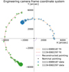 |
Fig. 1 Toy simulation of the positions of two stars in the vicinity of the Crab Nebula. The simulation starts where the highly populated reconstructed star positions are visible. Star identifiers correspond to the NOMAD catalog (Zacharias et al. 2005). |
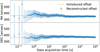 |
Fig. 2 Reconstructed pointing offset as a function of elapsed time since the start of the simulation determined from the two stars in Fig. 1. The error bars depict one standard deviation uncertainty on the fitted pointing offset, corresponding to the propagation of the single-star position reconstruction uncertainties. |
3.1 Variance images
A star provides a continuous light flux. The variance of the amplitude of such a signal is proportional to the count rate of detected photons. Thus, the brighter the star, the higher the variance of the pixel’s waveform that has the star in its FoV. To achieve good accuracy of the star reconstruction, the variance image of the camera (i.e. the snapshot of the camera with variance calculated for each pixel) must be properly cleaned. First of all, as we considered the physics data stream, some pixels would be affected by photons from extensive air showers (EASs) produced by cosmic rays or very high-energy gamma rays. Second, the night sky background (NSB) photons would introduce a Poisson noise. Due to the transient nature of the EAS, the probability that the same camera pixel will see the photons from the EAS in the majority of events in a set of N consecutive events is very small. Thus, we can use a clean-and-average approach to obtain a high-quality image of the star field with the following algorithm:
Take N consecutive events;
Clean each event from the EAS contamination by selecting only the pixels that are not affected by the EAS signals;
Produce a cleaned average variance image using all selected pixels from these events, and subtracting the average NSB contribution.
Below we provide a detailed description of each step of the algorithm presented above. We started with a calibrated events stream, where the pixel waveform amplitude is provided in photoelectrons (p.e.). The calibration of simulated data is trivial, and for observation data, we used the dedicated software provided by the LST Collaboration (Lopez-Coto et al. 2022). In order to clean an event from the EAS contamination, the LocalPeakWindowSum charge extraction algorithm (Kosack et al. 2022) was applied to each pixel to produce a reconstructed charge image. The window shift and width were set to 4 and 8 ns (default for LST-1). The pixels affected by EAS were then determined using the standard LST image reconstruction tools (Lopez-Coto et al. 2022; Kosack et al. 2022), using the default cleaning parameters2. The variances of the EAS-affected pixels were then replaced with the average NSB level, which was calculated using only the pixels selected according to the following criteria:
the pixel is not affected by the extensive air shower photons;
the pixel is not in the vicinity of the position where a star is expected to be reconstructed3;
the pixel is switched on with regular gain settings.
The last condition is specific to the PMT-equipped telescopes and is particularly relevant to the LST camera. In order to avoid damage to PMTs receiving too much light, from a car flash for example, their voltage is reduced to lower their gain when the drawn current surpasses a certain safety threshold. As an accurate calibration accounting for this gain change has not yet been implemented in the data analysis pipeline, these pixels were masked, and the stars containing them were not considered for the subsequent analysis.
The length of the averaging window must be optimized for better precision, accuracy, and monitoring rate. It should be large enough to smooth the event-to-event variations caused by extensive air showers and NSB fluctuations, but small enough to fulfill the star reconstruction frequency requirement: the star should not noticeably move during the averaging time window.
We simulated N = 300 consecutive events (diffuse proton-induced EAS with primary particle energy distributed between 10 GeV and 100 TeV with spectral index equal to −2.0) with a few typical stars to find the optimal averaging window size. We used sim_telarray (Bernlöhr 2008) software package to perform a detailed simulation of the telescope’s optical system and readout electronics. The telescope parameters correspond to the LST-1 parameters (LST Collaboration 2022), and the same optimization should be repeated for other telescopes. Details on the star signal reconstruction are provided in Sect. 3.3. The results of the simulation are shown in Fig. 3. We observe that for all simulated stars, we obtain a stable variance using N = 200 events, and therefore use it throughout the paper for the star position reconstruction. With the LST-1 typical event rate of 10 kHz, this corresponds to a star position update frequency of 50 Hz and an image integration time of 20 ms.
To summarize, we took 200 consecutive events, cleaned each of them, and computed the average variance image, as described above. The average variance image will contain brighter clusters where stars are observed over the NSB. Finally, we computed the camera average NSB contamination considering only the pixels that are not exposed to the bright stars and subtracted it from each pixel of the variance image.
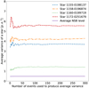 |
Fig. 3 Dependency of the average variance of the reconstructed star signal as a function of the number of consecutive events used in its computation. |
3.2 Point spread function effect on the star image
Seen at an infinite distance, a star would be imaged as a point in an ideal optical system. However, in real-life applications, the PSF alters the point-like image and needs to be accounted for. For a parabolic mirror composed of many facets, such as that mounted on the LST, the PSF is produced by the convolution of the effects of the facet aberrations. In addition, the I ACT’s optical system is not focused to infinity, but to the typical air shower development height. In the LST, the facet alignment is continuously monitored through an active mirror control system and corrected with motorized mirror actuators. Another dominating effect, entering the PSF and intrinsic to a parabolic mirror, is the coma aberration. It cannot be avoided, as light rays are not all parallel to the optical axis.
In order to determine the PSF shape, we performed a series of star simulations at different positions with respect to the pointing direction using the sim_telarray software package. While coma aberration was precisely simulated, the additional correction to the PSF due to imperfect mirror surface and facet alignment was extracted from PSF measurements performed with the specific LST-1 hardware. Figure 4 shows the spatial distribution of the photons caused by the PSF. In addition to the spreading effect, the reconstructed star position (a center of gravity of photon hits) is displaced from the expected position in the direction away from the optical axis proportionally to the distance between the expected star position and the optical axis of the system.
Using the simulations of stars in sim_telarray, we can model the PSF shape as a function of the expected star position. We express the positions of individual star photons in polar coordinates centered at the camera center. The choice of polar coordinates is motivated by the fact that the PSF is symmetric over the ϕ coordinate and is asymmetric over r. The starlight distribution (along the ϕ and r coordinates) can be parameterized with regular and asymmetric Laplace functions:
 (2)
(2)
for regular Laplace function and
 (3)
(3)
for asymmetric Laplace function.
Figure 5 provides an example of a PSF parametrization for one star position, simulated 0.8° away4 from the telescope’s optical axis. Good agreement is observed between the simulated ray tracing data (histograms) and the fitted PSFs (blue lines) for both angular and radial components.
With star simulations at different positions in the camera frame, we can establish an analytic dependence of the PSF parameters on the nominal star position. The L and ϕ0 parameters always correspond to the position of the PSF maximum in r and ϕ. Measured values of scale (SR, Sϕ) and asymmetry (K) parameters together with their analytical representations as a function of the radial distance are shown in Fig. 6. Due to the radial symmetry of the telescope, these parameters have no dependence on the polar angle, as confirmed by simulations. The error bars correspond to one standard deviation of the parameter along the polar angle. The dependence of the PSF parameters on the radial distance from the camera center can be described by analytical functions given in Eq. (4):
 (4)
(4)
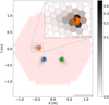 |
Fig. 4 Distribution of star photons in the LST-1 photodetection plane. The different colors indicate different simulated stars, and the grayscale corresponds to the distribution of the star photon hit probability per each camera pixel. The red dot in the zoomed section indicates the true simulated star position. |
3.3 Star position reconstruction and uncertainty
At this point, we are ready to describe the star position reconstruction. First of all, we identify all the bright objects in the telescope’s FoV using its nominal pointing and a catalog of stellar objects. The intensities of the signals from stellar objects observed in the telescope’s camera depend on their apparent magnitudes, the spectral response of the telescope (mirror, camera optical components, and sensors), the telescope readout settings, and the observation conditions. Ground-based IACT sensors are most sensitive in the 400–500 nm wavelength range, which makes it convenient to use the V-band optical magnitude to select stars from the catalog. Selected stars should be bright enough to be detectable, but not too bright to saturate the pixels. Furthermore, in the case of PMT-equipped cameras, the pixels that receive too much light will be turned off for protection. The typical optical magnitude range in V-band for the LST-1 telescope is between 4 and 7, as determined from observations5. The size of the queried sky patch is determined by the telescope FoV and constitutes 2° for the LST. While not every observation target will have enough “good” stars around it, 90% of the high-energy gamma-ray sources that can be observed from the CTA-North site have at least two stars in the right optical magnitude range and within a 2° cone around them. We show below that having two stars in the pointing reconstruction routine is sufficient to achieve the desired accuracy and precision.
Following the selection of the stars that can potentially be reconstructed, we proceed with the production of clean variance images following the steps described in Sect. 3.1. For each star, we form a cluster of camera pixels around its expected position in the Cherenkov camera frame. A pixel is added to the cluster if the integral of PSF over a given pixel’s area exceeds a predefined (configurable) threshold. From general considerations, we set this threshold to be 1% of the total PSF integral. The star is considered detected if at least one pixel of the cluster has a variance surpassing three standard deviations of the NSB-only variance. In order to reconstruct the star position, we calculate the weighted mean of the pixel center positions, using the pixel’s variance values as weights, and apply the radial scale factor to compensate for the radial shift induced by the PSF. The uncertainty on the reconstructed position is implemented as the covariance of the pixel’s center coordinates, using the per pixel integrated PSF values as weights. The performance of the single-star position reconstruction has been evaluated with simulations. A star is simulated as N photons randomly distributed over an area 1.2 times the telescope dish diameter and ray-traced to the camera. The number of photons is selected such that the variance of the simulated star signal corresponds to the variance observed in the real data. A position reconstruction accuracy of 20″ and precision of 25″ is observed for a star positioned 1° away from the telescope’s optical axis.
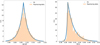 |
Fig. 5 PSF fit along the ϕ (left) and r (right) polar coordinates for the LST-1. |
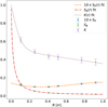 |
Fig. 6 Parameterizations of the PSF components as a function of the radial distance between the star and the camera center. |
4 Results
The most important feature of our method is that it requires neither additional hardware nor specific data taking conditions to be applied. It provides us with an opportunity of pointing accuracy monitoring for ongoing observations and for retrospective pointing analysis of the collected data.
To date, we have only performed a crude assessment of the achievable star tracking pointing reconstruction accuracy and precision based on a toy simulation. Prior to the method’s application to real data, we would like to estimate its performance using a detailed simulation of the potential physics observation.
4.1 Performance estimation on simulations
In order to make the simulations realistic, we tuned the simulation inputs to reflect a real observation run with the LST-1 telescope. We used the latest LST-1 telescope model which includes all the latest studies on the telescope’s camera, dish, and mirror characteristics, such as photomultipliers differential spectral sensitivity, point spread function6 and mirror reflectivity (LST Collaboration 2022). We did not simulate the extensive air showers because their impact on the star position reconstruction is negligible following the variance images cleaning and averaging procedures. Because the telescope simulation software, sim_telarray, does not simulate the telescope motion, we prepared a multitude of very short simulations, changing the telescope pointing (and simulated star positions) in steps of one second. Thus, the star positions were reconstructed at a rate of 1 Hz, and the telescope pointing was reconstructed at a frequency of 0.1 Hz. The NSB and star luminance contributions to the signal variance were extracted from the observation data. It should be noted that the simulated conditions correspond to the partial moon illumination, resulting in a tenfold NSB level increase to the nominal (dark night) NSB contribution. These conditions constitute the most challenging environment for star position reconstruction that can potentially be observed by the IACTs. Thus, we expected a fair estimation of the method’s performance and no degradation in the actual observing conditions.
We performed two simulations of the same observation block of approximately 2 h duration (covering the telescope zenith distance range between 15° and 40°) while virtually tracking the 13 Com star. The simulated positions of the stars are shown in Fig. 7. Since the simulation was carried out near the culmination of the stars’ diurnal arc trajectories, their apparent angular speed and traveled distances are small. The first simulation was performed with a perfect telescope’s pointing (see Fig. 8). The second simulation includes an artificially introduced variable pointing offset (see Figs. 9 and 10). The first simulation allows the estimation of the stability of the method and its potential accuracy, while the second determines the sensitivity of our star reconstruction algorithm to possible variable pointing offsets during observations. Figure 8 (top) shows that the reconstructed pointing offset is on average lower than 10″ and compatible with zero throughout the simulated observation block, as expected. A careful eye can spot the three somewhat distinct regions: [21:30-22:07], [22:08-22:46], and [22:47-23:15]. The small but recognizable shifts in the reconstructed pointing offset are due to the movement of stars across the camera pixels which changes the shapes of their clusters. To improve the reconstruction stability, we increased the cluster size by loosening up the pixel inclusion criterion: the integral PSF of the expected signal in the pixel can now be as low as 0.1%, rather than 1% (we call this a “loose” cluster). This allows more stable position reconstruction at the price of precision because a larger cluster potentially collects more noise. The results with this setting are shown in Fig. 8 (bottom). Nonetheless, the size of these shifts is much smaller than the typical size of the pixel, and so the reconstructed pointing precision is not much affected. In the following, we apply the loose cluster definition to all the simulated and observed datasets.
A slightly different picture appears in the case of the reconstruction of an artificially introduced progressive pointing offset of the telescope axis in Fig. 9. We shift all stars positions in the camera frame by adding 2.4″ for each degree of the telescope pointing motion in both zenith and azimuth directions. This increasing shift (−10″ to +40″ in zenith and −15″ to 15″ in azimuth) is comparable to the pointing offsets of the LST telescopes, which would still satisfy the tracking requirement of CTA. Figure 9 shows the comparison between the simulated and reconstructed pointing offset and Fig. 10 provides its decomposition in zenith and azimuth components. The accuracy of the pointing shift reconstruction is not uniform over the simulated time range. The accuracy in the zenith distance direction also appears to be superior to that in the azimuth direction. This difference can be attributed to the nearly parallel movement of the three fitted star clusters with respect to the zenith distance axis projection on the camera frame coordinate system. Combining this with the fact that the star’s cluster increases in size due to the degrading PSF in the off-axis direction, it becomes clear that the spread of the starlight over the zenith distance component is much larger than over the azimuth distance. This explains why we observe much better reconstruction accuracy in the zenith distance direction. Despite this limitation, the accuracy of the method remains very good and below 15″.
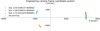 |
Fig. 7 Trajectories of simulated stars, corresponding to 13 Com tracking simulation between 21:30 and 23:15 on April 9, 2022. |
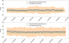 |
Fig. 8 Reconstructed and simulated pointing offset as a function of time for the perfect pointing simulation with “tight”(top) and “loose” (bottom) cluster definition. |
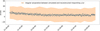 |
Fig. 9 Angular separation between simulated and reconstructed pointing offset as a function of time, for the simulation with the artificially introduced variable pointing offset with “loose” cluster definition. |
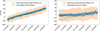 |
Fig. 10 Reconstructed zenith distance and azimuth components of a pointing offset as a function of time for the simulation with the artificially introduced variable pointing offset with “loose” cluster definition. |
4.2 Application to real data using the Large-Sized Telescope
Finally, we applied the star tracking method to the real data run used to set up the simulations described above. The data taking was performed by the LST-1 telescope installed at the Roque de los Muchachos Observatory at La Palma, Spain on April 9, 2022. The data analysis was performed with the same settings as used for the simulations. The only difference was the presence of the extended air showers in the observations as they played a triggering role in the data acquisition. Due to the nature of the LST-1 DAQ system, the data acquired by the telescope is written to the disk in small chunks called subruns. The typical duration of a subrun is about 5 s. While this data division is not significant for the star tracking method, it provides a convenient way of pointing reconstruction at the 𝒪(1 Hz) rate. Figure 11 presents the reconstructed pointing offset as a function of time, while Fig. 12 describes its zenithal and azimuthal components as a function of the zenith distance. The results are grouped according to the number of stars used in the pointing offset reconstruction. This number varies in time, due to transient phenomena such as car flashes or clouds in the FoV. For instance, the gap around 23:15 is caused by a flash of car lights, which is clearly visible in the camera images. We observe that one reconstructed star trajectory is insufficient to provide a stable unbiased pointing reconstruction. However, with two or more reconstructed stars our method demonstrates sufficient stability. The results show a maximum pointing offset smaller than 100″, which is close to the 60″ target tracking accuracy. A large structure, such as the LST telescope bearing a heavy camera and a large mirror dish, inevitably deforms due to gravitational forces. In addition to the elevation-dependent camera sagging, the mirror dish flattens out under its own weight, causing changes in the effective focal length and in the shape of the PSF, thus reducing the accuracy and precision of the single-star position reconstruction. During the commissioning period, the LST Collaboration worked on the telescope bending model and the corrections to the active mirror control settings. While the main effect had been properly compensated, final adjustments to the bending model were ongoing at the time the data for this study was acquired. Apart from the very high elevation angles (small zenith distance), the telescope pointing seems stable. One clearly outlying measurement is observed at around 8° of zenith. This behavior might be caused by two factors: an incorrect calibration of some of the camera pixels or an actual deviation of the telescope’s drive from the perfect trajectory. With the implementation of the interleaved calibration event analysis (pedestal and flat-fielding events), we expect to eliminate such outliers. Finally, residual overcorrection due to the bending model is observed together with a clear trend with the telescope elevation angle.
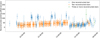 |
Fig. 11 Reconstructed pointing offset as a function of time with “loose” cluster definition, real data, observed with LST-1 on April 9, 2022. |
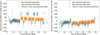 |
Fig. 12 Reconstructed zenith distance (left) and azimuth (right) pointing offsets with “loose” cluster definition as a function of telescope elevation, real data, observed with LST-1 from 21:30 to 24:00 on April 9, 2022. |
5 Conclusions
A pointing monitoring method that only relies on the analysis of the Cherenkov camera calibrated events has been developed. The accuracy and precision of the technique have been evaluated on dedicated Monte Carlo simulations and are of the order of 20″. The method can achieve pointing monitoring at frequencies up to 50 Hz, assuming a ≈10 kHz event rate. It has been applied to real data, and has proved to be remarkably stable (with the deviations not exceeding 20″) when at least two stars are used. In the application to the LST-1 data, it proved that the online pointing accuracy of 1′ is met. The method was designed to be available for all types of telescopes. While its precision and accuracy depend on each telescope’s configuration, better performance is expected with telescopes having a larger FoV, due to the potential increase in the number of stars that can be reconstructed. The method requires at least two stars in the FoV that are bright enough to be reconstructed, and not too bright to surpass the safety illumination level of camera pixels that causes a lowering of the gain of PMTs. This approach can work alongside regular data collection and can be utilized as a complementary tool for pointing monitoring in the CTA Observatory or other telescopes.
The star tracking method’s accuracy and precision can be further improved. The key factors affecting the method performance are precise camera calibration and a good understanding of the telescope’s PSF and its evolution as a function of the off-axis angle. The former can be addressed with a detailed analysis of the interleaved calibration events. The latter requires the off-axis PSF measurements with auxiliary devices and can be further improved by implementing signal pattern matching algorithms. These algorithms are computationally expensive and must be carefully considered and optimized before implementation to preserve a quasi-online pointing monitoring rate. Another interesting case of the star tracking method application is the monitoring of the PSF shape and the mirror alignment. These developments will be studied in detail and presented in future publications.
Acknowledgements
This work was conducted in the context of the CTA-LST Project. We gratefully acknowledge financial support from the following agencies and organizations: Ministry of Education, Youth and Sports, MEYS LM2015046, LM2018105, LTT17006, EU/MEYS CZ.02.1.01/0.0/0.0/16_013/0001403, CZ.02.1.01/0.0/0.0/18_046/0016007 and CZ.02.1.01/0.0/0.0/16_019/0000754, Czech Republic; Max Planck Society, German Bundesministerium für Bildung und Forschung (Verbundforschung / ErUM), Deutsche Forschungsgemeinschaft (SFBs 876 and 1491), Germany; Istituto Nazionale di Astrofísica (INAF), Istituto Nazionale di Fisica Nucleare (INFN), Italian Ministry for University and Research (MUR); ICRR, University of Tokyo, JSPS, MEXT, Japan; JST SPRING - JPMJSP2108; Narodowe Centrum Nauki, grant number 2019/34/E/ST9/00224, Poland; The Spanish groups acknowledge the Spanish Ministry of Science and Innovation and the Spanish Research State Agency (AEI) through the government budget lines PGE2021/28.06.000X.411.01, PGE2022/28.06.000X.411.01 and PGE2022/28.06.000X.711.04, and grants PGC2018-095512-B-I00, PID2019-104114RB-C31, PID2019-107847RB-C44, PID2019-104114RB-C32, PID2019-105510GB-C31, PID2019-104114RB-C33, PID2019-107847RB-C41, PID2019-107847RB-C43, PID2019-107988GB-C22; the “Centro de Excelencia Severo Ochoa” program through grants no. CEX2021-001131-S, CEX2019-000920-S; the “Unidad de Excelencia María de Maeztu” program through grants no. CEX2019-000918-M, CEX2020-001058-M; the “Juan de la Cierva-Incorporación” program through grant no. IJC2019-040315-I. They also acknowledge the “Programa Operativo” FEDER 2014-2020, Consejería de Economía y Conocimiento de la Junta de Andalucía (Ref. 1257737), PAIDI 2020 (Ref. P18-FR-1580) and Universidad de Jaén; “Programa Operativo de Crecimiento Inteligente” FEDER 2014-2020 (Ref. ESFRI-2017-IAC-12), Ministerio de Ciencia e Innovación, 15% co-financed by Consejería de Economía, Industria, Comercio y Conocimiento del Gobierno de Canarias; the “CERCA” program of the Generalitat de Catalunya; and the European Union’s “Horizon 2020” GA:824064 and NextGenerationEU; We acknowledge the Ramon y Cajal program through grant RYC-2020-028639-I and RYC-2017-22665; State Secretariat for Education, Research and Innovation (SERI) and Swiss National Science Foundation (SNSF), Switzerland; The research leading to these results has received funding from the European Union’s Seventh Framework Programme (FP7/2007–2013) under grant agreements nos. 262053 and 317446. This project is receiving funding from the European Union’s Horizon 2020 research and innovation programs under agreement no. 676134. ESCAPE – The European Science Cluster of Astronomy & Particle Physics ESFRI Research Infrastructures has received funding from the European Union’s Horizon 2020 research and innovation programme under Grant Agreement no. 824064.
References
- Adams, C. B., Alfaro, R., Ambrosi, G., et al. 2021, Astropart. Phys., 128, 102562 [NASA ADS] [CrossRef] [Google Scholar]
- Astropy Collaboration (Price-Whelan, A. M., et al.) 2022, ApJ, 935, 167 [NASA ADS] [CrossRef] [Google Scholar]
- Bernlöhr, K. 2008, Astropart. Phys., 30, 149 [CrossRef] [Google Scholar]
- Boggs, P. T., Spiegelman, C. H., Donaldson, J. R., & Schnabel, R. B. 1988, J.Econometrics, 38, 169 [CrossRef] [Google Scholar]
- Braun, I. 2007, PhD thesis, Combined Faculties for the Natural Sciences and for Mathematics of the Ruperto-Carola Univeristy of Heidelberg, Germany [Google Scholar]
- CANGAROO Collaboration (Hara, T., et al.) 1993, Nucl. Inst. Meth. Phys. Res., A332, 300 [NASA ADS] [Google Scholar]
- Cherenkov Telescope Array Consortium (Acharya, B. S., et al.) 2018, Sciencewith the Cherenkov Telescope Array (WSP) [Google Scholar]
- Iovenitti, S. 2022, PhD thesis, Milan University, Italy [Google Scholar]
- Kaplan, G. H. 2006, USNO-CIRC-179 (Washington: USNO) [Google Scholar]
- Kifune, T., Fujii, H., Fujimoto, M., et al. 1993, in Towards a Major Atmospheric Cherenkov Detector – II for TeV Astro/Particle Physics, ed. R.C. Lamb, 39 [Google Scholar]
- Kosack, K., Nöthe, M., Watson, J., et al. 2022, https://doi.org/10.5281/zenodo.6460868 [Google Scholar]
- Lopez-Coto, R., Vuillaume, T., Moralejo, A., et al. 2022, https://doi.org/10.5281/zenodo.6453871 [Google Scholar]
- LST Collaboration (K. Abe et al.) 2022, LST Prod2 v1.4 sim_telarray configuration https://github.com/cta-observatory/lst-sim-config/releases/tag/sim-telarray-lst-magic-prod2-v1.4 [Google Scholar]
- National Imagery and Mapping Agency 2000, Department of Defense WorldGeodetic System 1984: its definition and relationships with local geodeticSystems, Tech. Rep. TR8350.2 [Google Scholar]
- Nöthe, M., Kosack, K., Nickel, L., & Peresano, M. 2021, PoS, ICRC2021, 744 [Google Scholar]
- Pareschi, G. 2020, PoS, ICRC2019, 758 [Google Scholar]
- Segreto, A., Catalano, O., Maccarone, M. C., et al. 2019, in International CosmicRay Conference, 36, 36th International Cosmic Ray Conference (ICRC2019), 791 [NASA ADS] [Google Scholar]
- Yoshikoshi, T. 1996, PhD thesis, Tokyo Inst. Tech., Japan [Google Scholar]
- Yoshikoshi, T., Kifune, T., Dazeley, S. A., et al. 1997, ApJ, 487, L65 [NASA ADS] [CrossRef] [Google Scholar]
- Zacharias, N., Monet, D. G., Levine, S. E., et al. 2005, VizieR Online DataCatalog, I/297 [Google Scholar]
- Zaric, D., Cikota, S., Fiasson, A., et al. 2019, PoS, ICRC2019, 829 [Google Scholar]
All the telescopes of the CTA Observatory are expected to provide waveforms, and this feature is also included in the standardization of the raw event data model.
Picture threshold: 7; boundary threshold: 5; and no isolated pixels.
See Sect. 3.3 for the details of the pixel clustering around the expected star position.
In the case of the LST-1 telescope, this corresponds to a 0.39 m displacement in the camera frame coordinate system.
These are boundary values, corresponding to a dark night with good weather (optical magnitude 7) and high-NSB or challenging atmospheric conditions (optical magnitude 4).
The measurements of the off-axis PSF were not available at the time of this study.
All Figures
|
Fig. 1 Toy simulation of the positions of two stars in the vicinity of the Crab Nebula. The simulation starts where the highly populated reconstructed star positions are visible. Star identifiers correspond to the NOMAD catalog (Zacharias et al. 2005). |
| In the text | |
|
Fig. 2 Reconstructed pointing offset as a function of elapsed time since the start of the simulation determined from the two stars in Fig. 1. The error bars depict one standard deviation uncertainty on the fitted pointing offset, corresponding to the propagation of the single-star position reconstruction uncertainties. |
| In the text | |
|
Fig. 3 Dependency of the average variance of the reconstructed star signal as a function of the number of consecutive events used in its computation. |
| In the text | |
|
Fig. 4 Distribution of star photons in the LST-1 photodetection plane. The different colors indicate different simulated stars, and the grayscale corresponds to the distribution of the star photon hit probability per each camera pixel. The red dot in the zoomed section indicates the true simulated star position. |
| In the text | |
|
Fig. 5 PSF fit along the ϕ (left) and r (right) polar coordinates for the LST-1. |
| In the text | |
|
Fig. 6 Parameterizations of the PSF components as a function of the radial distance between the star and the camera center. |
| In the text | |
|
Fig. 7 Trajectories of simulated stars, corresponding to 13 Com tracking simulation between 21:30 and 23:15 on April 9, 2022. |
| In the text | |
|
Fig. 8 Reconstructed and simulated pointing offset as a function of time for the perfect pointing simulation with “tight”(top) and “loose” (bottom) cluster definition. |
| In the text | |
|
Fig. 9 Angular separation between simulated and reconstructed pointing offset as a function of time, for the simulation with the artificially introduced variable pointing offset with “loose” cluster definition. |
| In the text | |
|
Fig. 10 Reconstructed zenith distance and azimuth components of a pointing offset as a function of time for the simulation with the artificially introduced variable pointing offset with “loose” cluster definition. |
| In the text | |
|
Fig. 11 Reconstructed pointing offset as a function of time with “loose” cluster definition, real data, observed with LST-1 on April 9, 2022. |
| In the text | |
|
Fig. 12 Reconstructed zenith distance (left) and azimuth (right) pointing offsets with “loose” cluster definition as a function of telescope elevation, real data, observed with LST-1 from 21:30 to 24:00 on April 9, 2022. |
| In the text | |
Current usage metrics show cumulative count of Article Views (full-text article views including HTML views, PDF and ePub downloads, according to the available data) and Abstracts Views on Vision4Press platform.
Data correspond to usage on the plateform after 2015. The current usage metrics is available 48-96 hours after online publication and is updated daily on week days.
Initial download of the metrics may take a while.