| Issue |
A&A
Volume 679, November 2023
|
|
|---|---|---|
| Article Number | A17 | |
| Number of page(s) | 8 | |
| Section | Astrophysical processes | |
| DOI | https://doi.org/10.1051/0004-6361/202245259 | |
| Published online | 30 October 2023 | |
Improving the spin-down limits of the continuous gravitational waves emitted from rotating triaxial pulsars
Inter-University Centre for Astronomy and Astrophysics, Pune University Campus, Pune 411007, India
e-mail: This email address is being protected from spambots. You need JavaScript enabled to view it.
Received:
21
October
2022
Accepted:
18
July
2023
Abstract
The spin-down limit of the continuous gravitational wave strain from pulsars assumed to be triaxial stars rotating about a principal moment of inertia axis depends upon the value of the intrinsic spin frequency derivative of the pulsar, among other parameters. In order to get more accurate intrinsic spin frequency derivative values, dynamical effects contributing to the measured spin frequency derivative values must be estimated via more realistic approaches. In this work, we calculated improved values for the spin-down limit of the continuous gravitational wave strain (assuming that pulsars are triaxial stars rotating about a principal moment of inertia axis) for a set of 237 pulsars for which a targeted search for continuous gravitational waves was recently carried out by the LIGO-Virgo-KAGRA (LVK) Collaboration. We used ‘GalDynPsr’, a Python-based public package, to calculate more realistic values for the intrinsic spin frequency derivatives and, consequently, we get more realistic values of the spin-down limit. The realistic values that we obtain for the intrinsic spin frequency derivatives can also provide a valuable contribution to improving the sensitivity of searches for continuous gravitational waves from known pulsars.
Key words: gravitational waves / pulsars: general / stars: rotation
© The Authors 2023
 Open Access article, published by EDP Sciences, under the terms of the Creative Commons Attribution License (https://creativecommons.org/licenses/by/4.0), which permits unrestricted use, distribution, and reproduction in any medium, provided the original work is properly cited.
This article is published in open access under the Subscribe to Open model. This email address is being protected from spambots. You need JavaScript enabled to view it. to support open access publication.
1. Introduction
The measured values of pulsar parameters, such as spin frequency and its derivatives (fs, ḟs), are affected by the pulsar’s velocity and acceleration. These measured values hence contain contributions from additional terms that are functions of a pulsar’s velocity and acceleration (and even their derivatives) and are called the dynamical effect terms. A source of these dynamical effects that is common to all the pulsars in our Galactic field is the gravitational potential of the Milky Way (Pathak & Bagchi 2018).
While calculating parameters like the braking index (n) and the spin-down limit of the gravitational wave strain ( ), it is essential to use the intrinsic values of frequency derivatives, that is, ones that are devoid of any contamination from dynamical effects, in order to get more accurate results for these parameters.
The spin-down limit of the continuous gravitational wave strain from a pulsar assumed to be a triaxial star rotating about a principle moment of inertia axis is expressed as
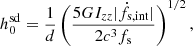 (1)
(1)
where ḟs,int is the intrinsic value of the spin frequency derivative, c is the speed of light in vacuum, G is the gravitational constant, d is the distance to the pulsar, and Izz is the z component of the moment of inertia.
Recently, Abbott et al. (2022) gave  values for 237 real pulsars. However, they only corrected for dynamical effects when calculating ḟs,int values for 144 pulsars out of the 237, and even here used a traditional approach (Damour & Taylor 1991) that does not work for pulsars further away from the Sun. In Sect. 2, we discuss the conventional approaches and their shortcomings, and suggest a more realistic approach to estimating the dynamical corrections to the spin period (or frequency) derivative of pulsars in order to estimate their intrinsic value, which is used in the calculation of
  values. In Sect. 3, we present our improved
  values based on ḟs,int values calculated using a Python-based package, ‘GalDynPsr’ (Pathak & Bagchi 2018), for the real pulsars in Abbott et al. (2022).
2. Estimating ḟs,int
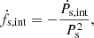
One can estimate ḟs,int from Ṗs,int by following the relation
 (2)
(2)
where Ṗs,int is the intrinsic value of the spin period derivative and Ps is the spin period.
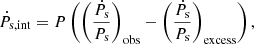
Ṗs,int can be estimated by subtracting from  the dynamical contributions to the observed value of the period derivative,
  (also called the excess term; see Pathak & Bagchi 2018), as shown in the following equation:
 (3)
(3)
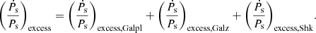
where we define the excess term,  , as
, as
 (4)
(4)
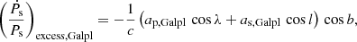
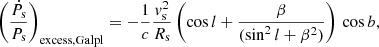
Here,  denotes the component of the excess term that contains the contribution from the component of relative acceleration parallel to the Galactic plane,
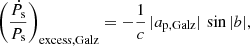
  denotes the component of the excess term that contains the contribution from the component of relative acceleration perpendicular to the Galactic plane, and
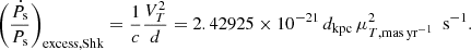
  denotes the component of the excess term that contains the contribution from the proper motion of the pulsar (also called the Shklovskii effect term; Shklovskii 1970). These components of the excess term are expressed as (Pathak & Bagchi 2018)
 (5)
(5)
 (6)
(6)
and
 (7)
(7)
In the above equations, l is the Galactic longitude, b is the Galactic latitude, d is the distance between the pulsar and the Solar System barycentre, ap, Galpl is the component of the pulsar’s acceleration parallel to the Galactic plane, as, Galpl is the component of the Sun’s acceleration parallel to the Galactic plane, ap, Galz is the component of the pulsar’s acceleration perpendicular to the Galactic plane, dkpc is the distance in kpc, VT is the total transverse relative velocity magnitude, and μT, mas yr−1 is the total proper motion in mas yr−1. cos λ is given by the relation 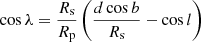 , in which Rs is the Galactocentric cylindrical distance of the Sun and Rp is the Galactocentric cylindrical distance of the pulsar, given by
  (Pathak & Bagchi 2018).
Conventionally, when estimating  , ap, Galpl and as, Galpl are taken to be centripetal accelerations, with
  and
and  , where vp is the Galactocentric rotational speed of the pulsar and vs is the Galactocentric rotational speed of the Sun parallel to the Galactic plane (Damour & Taylor 1991). Furthermore, vp is conventionally assumed to be a linear function of Rp with a negligible slope. In other words, pulsars are assumed to follow the flat rotation curve approximation (Damour & Taylor 1991; Reid et al. 2014). This leads to the use of an approximate expression,
 (8)
(8)
where 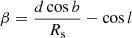 . However, the flat rotation curve approximation only works for the pulsars close to the Sun, that is, those which have Rp close to Rs, as the rotation curve is approximately flat for those Rp values. As we move away from the Sun, either towards the Galactic centre or towards the edges of the Galaxy, the rotation curve cannot be approximated by a flat line; hence, any estimation of
  using the flat rotation curve approximation is bound to give inaccurate results for such pulsars (Pathak & Bagchi 2018). Additionally, in Eq. (8), we can see that the dependence on the z value, that is, the vertical separation of the pulsar from the Galactic plane, is not taken into account.
Similarly, when estimating  , the approximate expressions for ap, Galz, given by Nice & Taylor (1995) as well as Lazaridis et al. (2009), have conventionally been used. In these expressions, ap, Galz only depends upon the z value and its magnitude tends to increase with the increase in vertical separation (Pathak & Bagchi 2018). This, we know, is counterintuitive, as moving away from the source of gravitational potential should eventually lead to a decrease in acceleration.
We know that acceleration is essentially the gradient of the gravitational potential. In a more realistic approach, therefore, the acceleration components in Eqs. (5) and (6) should be expressed in terms of gradients of the gravitational potential of the Milky Way. Specifically, ap, Galpl and as, Galpl should be estimated as the gradient of the Galactic potential along the Galactocentric cylindrical radial directions at the location of the pulsar and the Sun, respectively. ap, Galz, on the other hand, should be estimated as the gradient of the Galactic potential along the z direction at the location of the pulsar.
One such model for the Galactic potential is given in the publicly available Python package ‘galpy’ (Bovy 2015). It contains contributions from the Galactic disk, the central bulge, the dark matter halo, and the central supermassive black hole, and is referred to as ‘MWPotential2014wBH’. galpy also provides other Milky Way potential models like ‘MWPotential2014’ (the same as ‘MWPotential2014wBH’ except that it does not incorporate the contribution from the central supermassive black hole) and ‘McMillan17’ (which is based on the Milky Way potential given by McMillan 2017). However, the values of acceleration components calculated using these different Milky Way potential models are in agreement with each other for real pulsars (for details, see Pathak & Bagchi 2018; Bovy 2020). In this work, we used Model-Lb of GalDynPsr, which uses the ‘MWPotential2014wBH’ model from galpy for acceleration calculations, because, in addition to contributions from the Galactic disk, the central bulge, and the dark matter halo, we wanted to add the contribution from the central supermassive black hole for completeness. We discuss this in more detail in the following section.
3. Improving the h values of real pulsars: Correcting for dynamical effects in frequency derivatives
Tables 3 and 4 of Abbott et al. (2022) jointly give a list of  values for 237 real pulsars. They also provide the values of fs and Ṗs, which are used in the calculation of
  values. Out of these 237 pulsars, they corrected for the dynamical effects for only 144 pulsars. However, for these 144 pulsars, the dynamical effects corrected for include the Shklovskii effect (as given in Eq. (7)) and the Galactic rotation effect (as given in Eq. (8)), and hence, the
  and
and 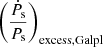 values were calculated but the
  values were not corrected for in Abbott et al. (2022). Moreover, the
  values were calculated using a flat rotation curve approximation, as given in Damour & Taylor (1991), which, as mentioned in the previous section, is not an accurate approach as it does not work for pulsars much further away from the Sun (Pathak & Bagchi 2018).
We therefore decided to use a Python package, ‘GalDynPsr’1 (Pathak & Bagchi 2018), to estimate more realistic ḟs,int (intrinsic spin frequency derivative) values for all the pulsars given in Abbott et al. (2022). We specifically used Model-Lb in GalDynPsr to calculate  and consequently ḟs,int. This model incorporates the use of the Milky Way potential ‘MWPotential2014wBH’, as given in galpy, to estimate the acceleration components required to calculate
  and
and  . GalDynPsr also calculates the Shklovskii effect contribution, that is,
  . Consequently, after having calculated the total dynamical contribution, that is,
  +
+  +
+  , GalDynPsr calculates the intrinsic value of the spin period derivative. In order to calculate ḟs,int using GalDynPsr, we required the values of the observable parameters: Galactic longitude (l), Galactic latitude (b), distance (d), proper motion in the right ascension direction (μα), proper motion along the declination (μδ), spin period (Ps), and the observed value of the spin period derivative (Ṗs,obs) (Pathak & Bagchi 2018).
For the observables l, b, μα, μδ, and ḟs,obs, we used the values given in version 1.70 of the ATNF pulsar catalogue (Manchester et al. 2005) for those 237 pulsars. For d and fs, we used the values given in Tables 3 and 4 of Abbott et al. (2022). For five of those pulsars, distance values are not available and so  values are not reported for these pulsars in Abbott et al. (2022). We dropped these five pulsars from our calculations as well and calculated
  values for the remaining pulsars using GalDynPsr.
Moreover, Abbott et al. (2022) found 13 pulsars (out of the remaining 232 pulsars) for which, after correcting for the dynamical effects, the Ṗs values turned out to be negative (Ṗs,int should be positive) and so  values are not reported by Abbott et al. (2022) for these pulsars either. However, for three (PSRs J1125+7819, J1300+1240, and J1832-0836) out of these 13 pulsars, we got a positive Ṗs,int value using GalDynPsr and so we calculated the
  value for these three. For the remaining ten pulsars (out of 13), we also got a negative value of Ṗs,int and we dropped those pulsars from our calculation of
  . After using GalDynPsr we found an additional five pulsars with negative Ṗs,int values and dropped these pulsars too from our calculation of
  .
.
For 77 of the 232 pulsars, proper motion values are not reported in the ATNF pulsar catalogue and so, for those pulsars,  does not have a contribution from
  . In the future, with improvements in timing precision, the proper motion values might be measured. Additionally, eight out of the 232 pulsars are globular cluster pulsars. For these pulsars, there will be an additional contribution to
  from the respective cluster potentials. Further investigation is required in order to calculate the respective cluster potentials and accelerations resulting from them, and hence, for both sets of pulsars discussed above (for which a complete contribution to
  is unavailable), after subtracting the available dynamical effects from the ḟs,obs values we actually got residual frequency derivative values (ḟs,res) instead of truly intrinsic frequency derivative values.
Finally, after ignoring the cases without distance measurements, with negative Ṗs,int values, without proper motion measurements, and those in globular clusters, we are left with 139 pulsars. Table A.1 contains the parameters for all these 139 pulsars. For five of these pulsars (indicated by superscript ϵ), Abbott et al. (2022) did not correct for dynamical effects. For 93 of the 139 pulsars, there is an increase in the ḟs,int values, implying an increase in  values when we compare the values calculated by us with those reported by Abbott et al. (2022). There are two pulsars (PSRs J2222-0137 and J1400-1431) for which the percentage increase in
  values is greater than 100%. For three pulsars (PSRs J2322-2650, J1709+2313, and J2010-1323), the percentage increase in
  values is between 20% and 100%. The first three rows of Table A.1 show the pulsars for which Abbott et al. (2022) got a negative Ṗs,int value and did not calculate
  , whereas we got a positive Ṗs,int value and calculated
  .
.
We note that Abbott et al. (2022) do not take into account errors in their estimation of the spin-down limits. We also do not provide error estimates as the Milky Way potential model that we use from galpy does not return errors in their potential and acceleration values. However, in the future, once we have a Galactic potential model that returns error values, it will not be a difficult task to incorporate that into GalDynPsr.
4. Conclusion
We know that for a pulsar to be a good candidate for the detection of continuous gravitational waves, that is, for it to be a high-value target, the ratio  should be less than one, where
  is the 95% credible upper limit of the gravitational wave amplitude, h0. Along with a precise measurement of
  , an accurate estimate of
  will improve the estimate of the ratio.
As mentioned previously, for calculating the  values using Eq. (1), ḟs,int values devoid of contamination from dynamical effects should be used. We used GalDynPsr to calculate the ḟs,int values for the pulsars given in Abbott et al. (2022).
We found that for two pulsars (PSRs J2222-0137 and J1400-1431) the percentage increase in  values was greater than 100% and for three pulsars (PSRs J2322-2650, J1709+2313, and J2010-1323) the percentage increase in
  values was between 20% and 100%. We also got a positive Ṗs,int value for three pulsars (PSRs J1125+7819, J1300+1240, and J1832-0836) using GalDynPsr, for which Abbott et al. (2022) got a negative value of Ṗs,int. We calculated the
  value for these pulsars too.
We suggest using Model Lb in GalDynPsr to calculate a more realistic value of ḟs,int before using it in the estimation of  (given the availability of all the required observables for estimating ḟs,int using GalDynPsr). For the pulsars present inside globular clusters, there will be an additional contribution from the respective cluster potentials to the
  term, and hence further investigation of cluster potential is required in order to calculate the true intrinsic value of the spin frequency derivative.
We know that pulsar distances are estimated through various methods, including from VLBI (Deller et al. 2013, 2018) or timing parallaxes (Bassa et al. 2016; Desvignes et al. 2016), from dispersion measure values using a model of free electron distribution in the Galaxy (such as the NE2001 model; Cordes & Lazio 2002, 2003), or from objects of known distance with which the pulsar has an association (such as globular clusters; Harris 1996). However, some methods are more accurate than others. Distances estimated from parallax values are generally more accurate than those measured using dispersion measure values. For example, the distance estimates for pulsars PSR J0437-4715 and PSR J1909-3744 are fairly accurate (based on timing parallaxes) and, for them, the percentage change in the  values was found to be −4.41% and 0.24%, respectively. In the future, with the increase in the number of parallax measurements of pulsars, their distance estimates will improve and using those estimates along with our formalism will give more realistic values of
  for those pulsars.
As a future scope of work, our method could turn out to be important for future gravitational wave searches. Using GalDynPsr, we got more realistic values of ḟs,int, which will improve the phase of the signal, as the phase evolution of the signal is dependent on the spin frequency and its derivatives. This may enhance the sensitivity of search pipelines for the continuous gravitational wave signals.
Acknowledgments
We are grateful to Prof. Wynn Ho for his suggestions and for drawing our attention to the recent work of Abbott et al. (2022). We would also like to thank the LIGO-Continuous Wave group, particularly Prof. Matthew Bailes, for their useful comments. We also thank Prof. Manjari Bagchi for her contribution to the formulation of GalDynPsr and for envisioning its applications. We are also grateful to Amy Hewitt and Cristiano Palomba for the information regarding the method used in Abbott et al. (2022) for the correction of dynamical effects.
References
- Abbott, R., Abe, H., Acernese, F., et al. 2022, ApJ, 935, 1 [NASA ADS] [CrossRef] [Google Scholar]
- Bassa, C. G., Janssen, G. H., Stappers, B. W., et al. 2016, MNRAS, 460, 2207 [NASA ADS] [CrossRef] [Google Scholar]
- Bovy, J. 2015, ApJS, 216, 29 [NASA ADS] [CrossRef] [Google Scholar]
- Bovy, J. 2020, arXiv e-prints [arXiv:2012.02169] [Google Scholar]
- Cordes, J. M., & Lazio, T. J. W. 2002, arXiv e-prints [arXiv:astro-ph/0207156] [Google Scholar]
- Cordes, J. M., & Lazio, T. J. W. 2003, arXiv e-prints [arXiv:astro-ph/0301598] [Google Scholar]
- Damour, T., & Taylor, J. H. 1991, ApJ, 366, 501 [NASA ADS] [CrossRef] [Google Scholar]
- Deller, A. T., Boyles, J., Lorimer, D. R., et al. 2013, ApJ, 770, 145 [NASA ADS] [CrossRef] [Google Scholar]
- Deller, A. T., Weisberg, J. M., Nice, D. J., & Chatterjee, S. 2018, ApJ, 862, 139 [NASA ADS] [CrossRef] [Google Scholar]
- Desvignes, G., Caballero, R. N., Lentati, L., et al. 2016, MNRAS, 458, 3341 [Google Scholar]
- Harris, W. E. 1996, AJ, 112, 1487 [Google Scholar]
- Lazaridis, K., Wex, N., Jessner, A., et al. 2009, MNRAS, 400, 805 [NASA ADS] [CrossRef] [Google Scholar]
- Manchester, R. N., Hobbs, G. B., Teoh, A., & Hobbs, M. 2005, AJ, 129, 1993 [Google Scholar]
- McMillan, P. J. 2017, MNRAS, 465, 76 [NASA ADS] [CrossRef] [Google Scholar]
- Nice, D. J., & Taylor, J. H. 1995, ApJ, 441, 429 [NASA ADS] [CrossRef] [Google Scholar]
- Pathak, D., & Bagchi, M. 2018, ApJ, 868, 123 [NASA ADS] [CrossRef] [Google Scholar]
- Reid, M. J., Menten, K. M., Brunthaler, A., et al. 2014, ApJ, 783, 130 [Google Scholar]
- Shklovskii, I. S. 1970, Soviet Astron., 13, 562 [NASA ADS] [Google Scholar]
Appendix A: Table
Parameters of the 139 pulsars for which all the required observables are available to calculate the complete dynamical effect contribution, using GalDynPsr to calculate the ḟs,int values. Here, l is the Galactic longitude, b is the Galactic latitude, d is the distance between the pulsar and the Solar System barycentre, μα is the proper motion in the direction of the right ascension, μδ is the proper motion in the declination, fs is the spin frequency, ḟs,obs is the observed value of the first derivative of the spin frequency, ḟs,int is the intrinsic value of the first derivative of the spin frequency,  is the spin-down limit of the pulsar (assumed to be a rotating triaxial star) calculated in this work,
  is the 95% credible upper limit of the gravitational wave amplitude h0, and
  is the spin-down limit of the pulsar (assumed to be a rotating triaxial star) as given in Abbott et al. (2022). The last column shows the percentage increase in the spin-down limit values. We display the results till the third decimal place. †: Pulsars for which Abbott et al. (2022) got a positive ḟs,int but we got a negative ḟs,int. ϵ: Pulsars for which the spin frequency derivative was not corrected for dynamical effects by Abbott et al. (2022).
All Tables
Parameters of the 139 pulsars for which all the required observables are available to calculate the complete dynamical effect contribution, using GalDynPsr to calculate the ḟs,int values. Here, l is the Galactic longitude, b is the Galactic latitude, d is the distance between the pulsar and the Solar System barycentre, μα is the proper motion in the direction of the right ascension, μδ is the proper motion in the declination, fs is the spin frequency, ḟs,obs is the observed value of the first derivative of the spin frequency, ḟs,int is the intrinsic value of the first derivative of the spin frequency, is the spin-down limit of the pulsar (assumed to be a rotating triaxial star) calculated in this work, is the 95% credible upper limit of the gravitational wave amplitude h0, and is the spin-down limit of the pulsar (assumed to be a rotating triaxial star) as given in Abbott et al. (2022). The last column shows the percentage increase in the spin-down limit values. We display the results till the third decimal place. †: Pulsars for which Abbott et al. (2022) got a positive ḟs,int but we got a negative ḟs,int. ϵ: Pulsars for which the spin frequency derivative was not corrected for dynamical effects by Abbott et al. (2022).
Current usage metrics show cumulative count of Article Views (full-text article views including HTML views, PDF and ePub downloads, according to the available data) and Abstracts Views on Vision4Press platform.
Data correspond to usage on the plateform after 2015. The current usage metrics is available 48-96 hours after online publication and is updated daily on week days.
Initial download of the metrics may take a while.