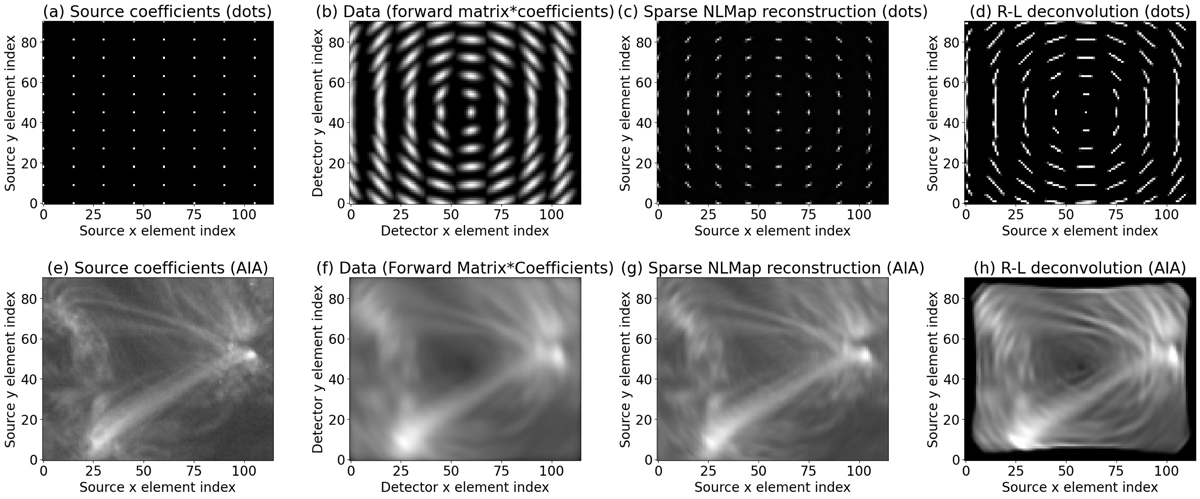
Two-dimensional example reconstructions with spatially varying PSF. Upper row: Test pattern of dots to show how the PSF appear. Panel a: Original pattern of dots. Panel b: Pattern with the PSF applied. Panel c: Pattern with the PSF and our correction algorithm. Here our algorithm is called “Sparse NLMap”, with “NL” standing for “nonlinear”. Panel d: Attempt to correct the data with a standard Richardson-Lucy (R–L) deconvolution. This approach does not incorporate a spatially varying PSF. With no noise and well-isolated features, resolution comparable to the original can be restored with our Sparse NLMap algorithm, but R–L fails to recover the original test pattern. Lower row: Application to AIA image also shown in Fig. 9 except at full rather than half AIA resolution. Panel e: Original image. Panel f: Image with varying PSF (same as upper panels) and noise applied. Panel g: Sparse NLMAP correction applied. Panel h: Attempt to correct with R-L. The reconstruction of AIA is much sharper and closer to the original source than the “data” is, although it is inevitably impacted somewhat by noise. The R–L deconvolution, on the other hand, shows many obvious artifacts of the variation and elongation of the PSF.