| Issue |
A&A
Volume 677, September 2023
|
|
|---|---|---|
| Article Number | A121 | |
| Number of page(s) | 14 | |
| Section | Numerical methods and codes | |
| DOI | https://doi.org/10.1051/0004-6361/202346914 | |
| Published online | 15 September 2023 | |
A deep learning approach for automated segmentation of magnetic bright points in the solar photosphere★
1
Yunnan Normal University, School of Information,
Kunming,
Yunnan
650500, PR China
e-mail: This email address is being protected from spambots. You need JavaScript enabled to view it.
2
Yunnan Normal University, School of Physics and Electronic Information,
Kunming,
Yunnan
650500, PR China
3
Key Laboratory on Adaptive Optics, Chinese Academy of Sciences,
Chengdu,
Sichuan
610209, PR China
4
Institute of Optics and Electronics, Chinese Academy of Sciences,
Chengdu,
Sichuan
610209, PR China
e-mail: This email address is being protected from spambots. You need JavaScript enabled to view it.
5
University of Chinese Academy of Sciences,
Beijing
100049, PR China
6
School of Electronic, Electrical and Communication Engineering, University of Chinese Academy of Sciences,
Beijing
100049, PR China
Received:
16
May
2023
Accepted:
4
July
2023
Abstract
Context. Magnetic bright points (MBPs) are small, bright, and conspicuous magnetic structures observed in the solar photosphere and are widely recognized as tracers of magnetic flux tubes. Previous studies have underscored the significance of MBPs in elucidating the mechanisms of coronal heating. The continuous advancement of solar telescopes and observation techniques has significantly enhanced the resolution of solar images, enabling a more detailed examination of MBP structures. In light of the growing availability of MBP observation images, the implementation of large-scale automated and precise MBP segmentation methods holds tremendous potential to facilitate significant progress in solar physics research.
Aims. The objective of this study is to propose a deep learning network called MBP-TransCNN that enables the automatic and precise pixel-level segmentation of MBPs in large quantities, even with limited annotated data. This network is designed to effectively handle MBPs of various shapes and backgrounds, including those with complex features.
Methods. First, we normalized our sample of MBP images. We then followed this with elastic deformation and rotation translation to enhance the images and expand the dataset. Next, a dual-branch encoder was used to extract the features of the MBPs, and a Transformer-based global attention mechanism was used to extract global contextual information, while a convolutional neural network (CNN) was used to extract detailed local information. Afterwards, an edge aware module was proposed to extract detailed edge features of MBPs, which were used to optimize the segmentation results. Focal loss was used during the training process to address the problem of the small number of MBP samples.
Results. The average values of precision, recall, F1, pixel accuracy, and intersection over union of the MBP-TransCNN are 0.976, 0.827, 0.893, 0.999, and 0.808, respectively. Experimental results show that the proposed MBP-TransCNN deep learning network can quickly and accurately segment the fine structure of MBPs.
Key words: techniques: image processing / Sun: photosphere / methods: observational
All the code and datasets used in this study have been made publicly available and can be accessed at the following link: https://github.com/yangpeng6/MBP-TransCNN
Haicheng Bai is the co-first author of the article.
© The Authors 2023
 Open Access article, published by EDP Sciences, under the terms of the Creative Commons Attribution License (https://creativecommons.org/licenses/by/4.0), which permits unrestricted use, distribution, and reproduction in any medium, provided the original work is properly cited.
This article is published in open access under the Subscribe to Open model. This email address is being protected from spambots. You need JavaScript enabled to view it. to support open access publication.
1 Introduction
Magnetic bright points (MBPs) are small, observable bright magnetic structures in the solar photosphere. Typically appearing in intergranular lanes, MBPs are the result of continuous interaction between magnetic flux tubes and the photosphere and are thus considered to be the footpoints of magnetic flux tubes (Berger et al. 1998; De Pontieu 2002; Yang et al. 2016). When pushed into intergranular lanes, MBPs oscillate under the jittering of granules, exciting magnetohydrodynamic (MHD) waves that propagate through the flux tubes and transfer energy to the chromosphere and lower corona, heating these regions of the solar atmosphere (Jess et al. 2009; Fedun et al. 2010; Vigeesh et al. 2012; Mumford & Erdélyi 2015; Mumford et al. 2015; Gao et al. 2021). Recent studies by Hofmeister et al. (2019) and Magyar et al. (2021) have elucidated the intricate linkage between MBPs and the footpoints of prominent atmospheric structures, such as coronal holes. Furthermore, these investigations have proposed the intriguing possibility that MBPs may serve as viable source regions for the newly detected phenomenon of magnetic switchbacks in the solar wind. Therefore, MBPs play a critical role in the study of various active behaviors of magnetic elements in the photosphere and in explaining coronal heating. With the development of ground-based solar telescopes and adaptive optics systems, the resolution of solar images has been increasing, revealing finer structures of MBPs. With the increasing number of observations of solar images, the automatic and accurate identification and segmentation of MBPs has become an important prerequisite for studying MBPs.
There are mainly two types of existing methods for identifying MBPs: traditional techniques and deep learning methods. Typical traditional approaches use the Laplacian operator combined with region growing or morphological methods, or they use intensity gradients to determine MBPs. Crockett et al. (2009) used computed intensity gradients in multiple directions to determine MBPs, followed by a region growing algorithm to obtain the recognized MBP size. Feng et al. (2012) first calculated candidate seed regions using the Laplacian operator, then used morphological methods to obtain the edge and size of MBPs. Xiong et al. (2017) proposed an edge detection and tracking method to detect MBPs followed by 3D methods for region growing. Liu et al. (2018) used the Laplacian operator as the seed for region growing to detect MBPs. Saavedra et al. (2022) segmented MBPs using multiple threshold values.
In addition to these typical MBP recognition techniques, deep learning methods have also been used for MBP recognition and segmentation in recent years. Yang et al. (2019) proposed a convolutional neural network (CNN) based on backpropaga-tion for morphological classification of small-scale MBPs. Xu et al. (2021) proposed a CNN based on tracking regions to identify MBPs, which was used to match the properties of isolated MBPs in multiple wavelengths.
Magnetic bright points are usually divided into isolated bright points (IBPs) and non-isolated bright points (NIBPs). The IBPs represent bright points that do not merge with or split into several bright points during their lifetime, while NIBPs do the opposite. In terms of morphology, IBPs are point-like, while NIBPs are elongated and knee-shaped or flower-shaped (Dunn & Zirker 1973; Berger et al. 1995; Müller et al. 2000; Abramenko et al. 2010; Xiong et al. 2017; Yang et al. 2019).
In recent years, many detection methods for MBPs have been developed using traditional image processing techniques. These methods have achieved good detection results by identifying MBPs from solar images based on gradients, intensity gradients, and other features. While these methods work well for isolating MBPs, they are less effective at segmenting complex non-isolated MBPs.
There are several reasons for this. First, the shapes of non-isolated MBPs vary and their edges are often unclear, making fine-grained segmentation difficult. Second, some of the granulation edges have high gradient values, making it challenging for traditional methods to exclude false positives. To address these challenges, traditional methods often use restrictions such as size thresholds (Utz et al. 2009), peripheral darkness (Yang et al. 2014; Xiong et al. 2017), and the Τ = aγ + bδ formula (where γ and δ represent the image’s mean and variance, and a and b are empirical values) to calculate the threshold for binary segmentation of the Laplacian image. However, these methods may be inaccurate for certain image data, and seed selection in region growing methods can lead to either missed or extra detections.
Yang et al. (2019) and Xu et al. (2021) have used the deep learning methods of Mask Region-based Convolutional Neural Network (Mask RCNN; see Appendix A; He et al. 2017) to train networks on manually annotated datasets of hundreds of MBPs. They achieved good segmentation accuracy using Mask RCNN to segment MBPs in G-band and TiO-band images. However, as the abundance of astronomical image data is substantial and MBPs are often small and have complex shapes, making manual annotation is time consuming and costly. In addition, the prediction speed of deep learning methods is relatively slow, at around 15 s per frame.
To address these issues, this paper proposes a deep learning MBP recognition and segmentation method based on a mixed encoder of CNN and Transformer (see Appendix A). The approach we propose has four main contributions: (1) To achieve effective learning on a small number of annotated images, we designed a Transformer branch in the hybrid encoder architecture with CNN that extracts global attention and then performs feature fusion with the initial network branch in order to enhance global semantic information. (2) The boundary between MBPs and the background is often fuzzy and challenging to discern, making it difficult to accurately localize the boundaries of MBPs without introducing additional prior information. Existing methods often struggle to achieve complete segmentation of MBP boundaries. To address this issue, we integrated an edge aware module (EAM) into the encoder structure to extract edge details from the image and enhance the precise segmentation of MBP boundaries. (3) To address the challenge of having only a small proportion of pixels being occupied by MBPs in the image, we used a weighted loss that assigns a larger training weight to the positive samples of MBPs and a smaller weight to the negative samples of the background. (4) To address the challenge of limited solar MBP image data, which requires a large amount of annotated data for deep learning training, we annotated only ten frames of the original dataset and generated a substantial number of synthetic images using data augmentation techniques. Elastic deformation was applied to the annotated dataset, which is particularly crucial for solar image segmentation, as this type of deformation is well-suited for solar images, and the deformed images still bear resemblance to the original real solar images.
The purpose of this article is to apply deep learning techniques in image processing to MBP segmentation. Deep learning networks have achieved state-of-the-art results in various fields due to their powerful learning abilities. This article presents the first attempt to mix CNNs and Transformers for precise pixel-level segmentation of MBPs.
The organization of this article is as follows. Section 2 provides a detailed description of the data, including the dataset and how to augment it. Section 3 introduces in detail the method of using the combination of CNN and Transformer to train the MBP segmentation network. Section 4 presents the experimental results of this method. Section 5 concludes the article by summarizing the method presented in Sect. 4.
2 Datasets and preprocessing
Deep learning methods require large annotated datasets for network training. In the process of deep learning, or machine learning, data are the main driving force for the model. By training with existing data, we obtain corresponding network parameters, allowing our designed model to have a generalized ability to predict unknown or unseen samples. Applying these parameters to practical applications is the main process of model training. The cleanliness, completeness, and other aspects of the data are critical factors affecting the quality of network learning. Therefore, the establishment of our MBP dataset is crucial and directly impacts the final segmentation performance.
2.1 Dataset
In this article, observational data from the 1.6-m aperture Goode Solar Telescope (GST) at the Big Bear Solar Observatory (BBSO; Cao et al. 2010) were used to segment solar MBPs. This telescope is equipped with an adaptive optics system that can accurately correct atmospheric distortions to obtain clear images. Imaging observations of the photosphere were performed using a broadband filter imager (BFI) and a TiO bandpass filter with a wavelength of 705.7 nm and a field of view occupying the central 70″ × 70″ of the solar disk (Anđić et al. 2011). The exposure time for each frame was 2 ms, with a frame cadence of 15 s. The TiO bandpass is widely used in the study of MBPs and sunspots. The observational data and observation logs from GST can be requested for download1.
Parameters of six datasets.
2.2 Building the dataset
We utilized observational data from six distinct time periods captured in the quiet region of the Sun. We processed these observational data using Bai (2022) normalization method and subsequently stored them as three-channel images. Table 1 lists the relevant details of these datasets.
We selected D1 as our training dataset, which corresponds to a day of quiet solar observations. This day was chosen to include variations in lighting conditions and a diverse range of clear MBP configurations. This selection is particularly effective in training a robust network that can handle various possible morphologies of MBPs. To ensure coverage of the observed data quality for most of the MBPs on that day, we included a temporal dimension in the selection of the training dataset. We curated a testing dataset comprising D2, D3, D4, D5, and D6, encompassing MBP observations from five distinct dates. The purpose of this selection is to showcase the robust performance of our algorithm across the majority of quiet solar regions while ensuring the preservation of MBP quality. These datasets span various time intervals, with some capturing shorter periods and others spanning more extended durations. The chosen images exhibit a diverse range of characteristics, encompassing instances with abundant MBP group formations as well as those featuring only a few instances. Furthermore, the image quality varies from blurry to clear. This comprehensive dataset encompasses a wide spectrum of observed MBP qualities. The successful identification and segmentation results achieved with this diverse collection of images serve as a testament to the efficacy of our algorithm.
To ensure high accuracy of the Ground Truths, the dataset utilized in this study was constructed by combining the detection results obtained from the algorithm of Bai (2022) with the expertise of several domain specialists. Specifically, building upon the identification performed by the Bai (2022) algorithm, our team of three domain specialists conducted further refinement to achieve highly accurate annotations. Regarding the identification outcomes, if two or more experts agreed on classifying a pixel as an MBP, we made the pixel white using Photoshop. Conversely, if two or more experts deemed a pixel to not be an MBP, we made it black. After annotating ten frames from the datasets, we expanded the dataset using elastic deformation. The steps for elastic deformation are as follows.
(a) Creating a random displacement field: Randomly generate two displacement fields ∆x(x,y) = rand(−1,+1) and ∆y(x,y) = rand(−1, +1) of the same size as the original image where each value at each position is a random number between −1 and 1. (b) Applying Gaussian convolution to the displacement field: Use a Gaussian kernel to convolve the displacement field to simulate small distortions and deformations that may exist in the image. The size of the convolution kernel is determined by a standard deviation parameter σ. The value of σ is determined by multiplying the width of the image by 0.08. After convolution, the values of the displacement field become smoother and more continuous. (c) Controlling deformation intensity (degree): multiply the displacement field by a scaling factor α to control the intensity (degree) of elastic deformation. The value of α is obtained by multiplying the width of the image by two. (d) Applying affine transformation to the image: apply affine transformation to the original image, including translation, rotation, scaling, and so on, to increase the degree of variation of the image. The parameters of the transformation matrix are randomly generated. The boundaries of the transformed image will have values that mirror the values near the original boundaries. The range of variation for the scaling parameters of the two axes is (−51.2, 51.2). (e) Applying the displacement field: apply the elastic deformation displacement field to the image after affine transformation to achieve elastic shape changes. For each pixel, move its position to the corresponding position in the displacement field and interpolate based on the values of neighboring pixels. (f) Returning the interpolated image: The image that has undergone deformation and affine transformation has greater variability and can be used as augmented data.
For a more comprehensive understanding of elastic deformation, readers can refer to the paper by Simard et al. (2003). The outcomes of elastic deformation are illustrated in Fig. 1. Eventually, we augmented the D1 dataset by transforming ten annotated images into 1000 via elastic deformation and used them as the training set for the network training.
3 Methods
In this study, our aim is to predict the H × W feature map of a high-resolution image with MBPs, having a spatial resolution of H × W and C channels, on a pixel-by-pixel basis. In the context of images, H refers to height, W represents width, and C denotes the three color channels of the image. Unlike conventional approaches that either utilize CNNs to directly encode images into high-resolution feature maps or utilize Transformers to encode images, our proposed method combines Transformers with CNNs. Specifically, in the encoder module, we leverage a Vision Transformer branch (ViTA) and a Vision Transformer hybrid CNN-Transformer branch (ViTB) to integrate high-level semantic information with low-level features. Additionally, we introduce an Edge aware module (EAM), which is simple yet effective, to incorporate low-level local edge information and high-level global positional information under explicit boundary supervision. This module enables us to explore the edge semantics related to object boundaries and helps us achieve accurate segmentation results.
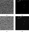 |
Fig. 1 Elastic deformation of the image and the result. (a) Original image of the MBP. (b) Binary image labeled MBP. (c) Original image after elastic transformation. (d) Binary image of the same labeled image after the same elastic deformation. |
3.1 MBP-TransCNN
To improve the segmentation of fine MBPs in complex data with limited visibility, we propose a novel dual-branch encoder network architecture. This architecture extracts both local low-resolution features of MBPs and global contextual information at each stage. To enhance the global modeling capability of the Transformer, we utilize a dual-branch encoder with parallel Transformers and Trans-CNN. This approach uses the CNN as a feature extractor and extracts patches from the feature map obtained from the CNN rather than from the original image, which helps model the global context of the image. In addition, to address the challenge posed by blurry edges and the difficulty in fine-grained segmentation of MBPs, we incorporated an EAM into our approach. The EAM module utilizes high-level semantic features as auxiliary information and exploits the spatial information to facilitate the exploration of edge-related features of these small objects (i.e., MBPs). The primary purpose of the EAM module is to provide valuable edge priors for the subsequent segmentation, enabling the network to better delineate the contours of these tiny and complex objects.
We chose this dual-branch design in order to use the intermediate high-resolution feature maps of the CNN, which can be combined in the decoder with high-level semantic information and low-level features for better segmentation performance. The proposed architecture is shown in Fig. 2, which includes the cascaded upsamplers for refining the segmentation results. By leveraging the self-attention mechanism of the Transformer, our proposed approach can model global, dynamic receptive fields and extract both local and global features, which can lead to improved MBP segmentation performance.
Decoder. To decode the hidden features and output the final segmentation mask, we used the cascaded upsampler (CUP) proposed in the TransUNet (Chen et al. 2021), which consists of multiple upsampling steps. After reshaping the hidden fea-ture sequence  into
into  represents the side length of the image patch, and the embedding dimension D can be obtained by calculating P2 × C, which is the product of the area of the image patch and the number of channels. The cascaded upsampler is instantiated through multiple cascaded upsampling blocks to achieve full resolution from
  to H × W, where each block consists of a 2× upsampling operator, a 3 × 3 convolution layer, and a Rectified Linear Unit (ReLU; see Appendix A) layer in that sequence. As shown in Fig. 2, this architecture achieves feature aggregation at different resolution levels by concatenating the features extracted by the CNN with the features upsampled by the dual-branch encoder via skip connections. The detailed architecture of CUP and the intermediate skip connections are shown on the right side of Fig. 2.
3.2 Transformer branch encoder
3.2.1 Transformer as encoder
Image sequentialization. In accordance with Dosovitskiy et al. (2020), we first input an H × W × C. We then transformed the image into a sequence of flattened two-dimensional blocks, denoted by xp ∈ N × (P2 × C), where C represents the number of channels in the image, each patch is of size P × P, and  is the number of image patches (i.e., the input sequence length). Each xp corresponds to a (P2 × C)-dimensional block, and the total number of such blocks is (H × C)/P2.
Patch embedding. To convert the flattened two-dimensional block sequence of xp ∈ N × (P2 × C) into the desired input matrix of size (N, D) required by Transformer, we performed a patch embedding operation. This operation applies a linear transformation to each vector, compressing the dimensions of the block sequence into D. To capture spatial information about each block’s location, we also learned location-specific embeddings, which are added to the block embeddings to encode position information as follows:
![Mathematical equation: ${Z_0} = \left[ {x_p^1E;x_p^2E; \ldots ;x_p^nE} \right] + {E_{{\rm{pos}}}},$](/articles/aa/full_html/2023/09/aa46914-23/aa46914-23-eq5.png) (1)
(1)
where E is a linear transformation (i.e., a fully connected layer),  ; the input channel is P2 · C; the output channel is N; and Epos ∈ ℝN×D denotes the position embedding.
The Transformer encoder consists of L layers of multihead self-attention (MSA) and multi-layer perceptron (MLP) blocks (Eqs. (2) and (3); see Appendix A). Therefore, the output of the ℓth layer can be written as follows:
 (2)
(2)
 (3)
(3)
where LN (·) is Lay er norm, after which the residual connection is applied at each block, and Zℓ is the image representation encoding. The structure of the Transformer layer is shown in Fig. 3. In our study, both ViT_A and ViT_B in Fig. 3 are composed of 12 such transformer layers.
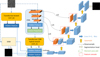 |
Fig. 2 Overview of the framework of the proposed MBP-TransCNN. |
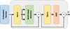 |
Fig. 3 Schematic of the Transformer layer. |
3.2.2 Edge aware module
Effective edge detection is crucial for accurate segmentation and localization in target detection. However, while lower-level features may contain rich edge details, many non-object edges may also be present. The presence of noise in these low-level features can make accurate detection difficult. To address this issue, the EAM module leverages high-level semantic features to aid in the exploration of edge features related to the target object. By promoting the exploration of such features, the EAM module provides valuable edge priors for subsequent segmentation and helps the network better segment the edge profiles of small, complex objects such as MBPs.
To achieve this, the input image is first convolved and reshaped to generate both low-level features (as shown in Fig. 3) and high-level features from a Vision Transformer model (ViTA), as illustrated in Fig. 4. The low-level features are extracted through a combination of 7 × 7 and 1 × 1 convolutions and reshaped into blocky features. The convolu-tional features are then concatenated with the advanced features from the ViTA model and passed through a sigmoid function to generate the edge feature fe. The EAM module is a simple and efficient method for extracting specific edge features, as demonstrated in Fig. 4, where EAM effectively learns the edge semantics associated with object boundaries. The dice loss was chosen as the marginal loss function in this module.
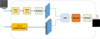 |
Fig. 4 Schematic diagram of EAM. EAM is designed to excavate marginal features related to small target objects. |
3.2.3 Focal loss
Focal loss is another solution to address the problem of imbal-anced MBP samples from the perspective of loss function Lin et al. (2020). From Fig. 1, it can be seen that the proportion of MBPs to all pixels is small. The specific form of Focal loss is
 (4)
(4)
 (5)
(5)
In practice, we consolidate an αt-balanced variant of the Focal loss expression into a unified formulation
 (6)
(6)
The parameter αt is the balancing factor that adjusts the contribution of each class based on its rarity or importance. The variable y takes values of one and zero, representing the foreground and background, respectively. Meanwhile, the variable p ∈ [0, 1] denotes the model’s estimated probability for the class labeled as y = 1, indicating the predicted probability of belonging to the foreground class.
The parameter γ ranges from zero to five and is used to reduce the contribution of easy samples to the loss function, thereby increasing the proportion of difficult samples. When pt approaches one, indicating that the sample is easy to distinguish, the modulation factor tends to zero, indicating that the contribution to the loss is small, which in turn reduces the proportion of easy samples. Conversely, when pt is very small, indicating that a sample is classified as a positive sample but the probability of being in the foreground is very small, it is misclassified as a positive sample. At this time, the modulation factor tends to one, and the impact on the loss function is not significant.
The parameter αt is used to suppress the imbalance in the number of positive and negative samples, and γ is used to control the imbalance between simple and difficult samples. Based on the proportion of positive samples occupied by MBPs and repeated experiments, we set αt to 0.95 and γ to two in this paper.
3.3 Training and testing
We used our improved Transformer and CNN hybrid encoding model, called MBP-TransCNN, for MBP segmentation based on Transformer and Resnet-50 (He et al. 2016). The MBP-TransCNN was deployed using a PC with RTX 3090 (24 GB device RAM) for training and testing. In the design of the hybrid encoder, we combined ResNet-50 and ViT to create “R50-ViT”. All transformer backbones (i.e., ViT) and ResNet-50 (denoted as “R-50”) were pre-trained on ImageNet (Deng et al. 2009). To reduce training time, we used the Chen et al. (2021) pre-trained network as the base point for training. The input resolution and patch size P were set to 224 × 224 and 16, respectively. Afterwards, we input a resolution of 640 × 640 into our proposed model and trained it with the Stochastic gradient descent (SGD) optimizer at a learning rate of 0.01, a momentum of 0.9, and a weight decay of 1 e-4. The default batch size was one, and the dataset contained 1000 images. The total number of training iterations for 100 epochs was 100 000. We refer to our trained network as MBP-TransCNN. The loss value stabilized after 10k iterations, which took approximately 9 h of training time.
To evaluate the segmentation performance of our network, we used five evaluation metrics for image segmentation in order to quantify the segmentation performance (Long et al. 2015). These metrics are precision, recall, F1 score, pixel accuracy (PA), and intersection over union (IoU). To calculate the above indicators, TP, TN, FP, and FN were required. The definitions of these terms are as follows: true positive (TP) is the number of pixels that are predicted to be positive and are actually positive. True negative (TN) is the number of pixels that are predicted to be negative and are actually negative. False positive (FP) is the number of pixels that are predicted to be positive but are actually negative. False negative (FN) is the number of pixels that are predicted to be negative but are actually positive.
In our dataset, there are two classes (0, 1), where zero represents the background and one represents MBPs. We used Ρii to represent the number of samples that are originally in class i and are predicted as class i, which corresponds to TP and TN. Next, Pijrepresents the number of samples that are originally in class i but predicted as class j, which corresponds to FP and FN. If class i is the positive class, then Ρii represents TP, Pjj represents TN, Pij represents FP, and Pij represents FN when i = j.
Pixel accuracy means to predict the proportion of pixels with correct categories in the total number of pixels. The calculation formula is as follows:
 (7)
(7)
Recall is the proportion of the predicted positive sample and the true positive sample out of all the true positive samples. In general, the higher the recall, the more positive samples that will be correctly predicted by the model and the better the model’s effect will be. The formula is  .
.
Accuracy, also known as precision, measures the accuracy of a model in predicting positive samples. The higher the accuracy, the greater the probability that the true label will also be positive in the predicted positive samples. The calculation formula is  .
.
The F1 score is a combination of the recall and precision, and it can reflect the model's ability to search accurately and comprehensively. The calculation formula is as follows:
 (8)
(8)
The intersection over union ratio representation refers to the ratio of intersection and union of predicted results and real values of a certain category. For image segmentation, it is found by calculating the intersection ratio between the predicted mask and the real mask. The calculation formula is  .
.
Table 2 presents the average PA, recall, F1 score, and IoU for MBP segmentation in five datasets. The mean values of precision, F1 score, and PA are all greater than 0.9, with the average values of precision, F1 score, and PA being 0.999, 0.920, and 0.963, respectively. We note that we employed pixel-level IoU, which is more accurate and sensitive to pixel changes, making it particularly suitable for detecting small objects such as MBPs. The recall and IoU are 0.887 and 0.854, respectively. These high accuracy metrics demonstrate the satisfactory performance of MBP-TransCNN in MBP detection and segmentation.
3.4 Detection and segmentation of MBPs
Our trained MBP-TransCNN network performed well on datasets D2–D6, exhibiting excellent segmentation results for MBP images. As shown in Fig. 5, each bright point is marked with a white label on a binary image, and the corresponding TiO-band image with bright points is labeled in green. The pixel-wise segmentation has segmented MBPs with clear boundaries.
Testing metrics.
4 Experimental results
In this experiment, we utilized TiO-band images obtained from the Big Bear Solar Observatory on multiple dates, including 2018 June 7, 2019 June 18, 2019 June 24, 2020 July 18, and 2021 April 30. Then, we used the dataset to conduct ablation experiments, comparative experiments, and robustness experiments. These three sets of experiments are presented in Sects. 4.1 and 4.2. All training experiments were performed on a single computer equipped with an RTX 3090 GPU and a memory capacity of 24 GB. All testing experiments were carried out on another single computer featuring a GTX 1660 GPU with a memory capacity of 6 GB.
4.1 Ablation experiments
In Sect. 4.1.1, we discuss how we trained a Transformer network with only a serial structure and compared its performance with that of a network with an additional Transformer branch (Sect. 3.2.1). In Sect. 4.1.2, we present a comparison of the performance of a network with an EAM edge guidance module and a network without an edge guidance module. In these ablation experiments, we used the same annotated data and training hyperparameters, that is, 100 training epochs, a learning rate of 0.01, and a batch size of one.
4.1.1 Branch encoder
In Fig. 6, we present the segmentation results of a dual-branch network and a single-branch network on three images captured at different time intervals. By extracting features using the dual-branch network, some of these large MBPs were fully recognized as correct shapes of MBPs. Due to the global attention mechanism of the transformer, not only were local MBPs taken into account but also the entire image during feature extraction. As a result, the misclassified MBPs were adjusted to their correct segmentation areas, as illustrated in the yellow and red box in Fig. 6, allowing the network to better segment MBPs with complex shapes. The improved segmentation performance of the model with the transformer branch is evident.
4.1.2 Edge aware module
Figure 7 shows the segmentation results with and without the EAM (Sect. 3.2.2) in the MBP-TransCNN network. The first column displays the prediction results of the MBP-TransCNN network with the EAM operation introduced in Sect. 3.2.2, while the second column shows the segmentation results without any operations for MBP segmentation. Figure 7 reveals that some edges of misdetected MBPs were correctly identified as correct edges when using the EAM. This is because the edges of some MBPs are extremely close to the intensity and grayscale of dark channels, making it difficult to distinguish between the two. It is difficult to achieve ideal segmentation results for these confusing and difficult-to-distinguish areas without some methods. However, the EAM contains prior knowledge of the edges of MBPs and achieved a fine segmentation of the edges, as much as possible.
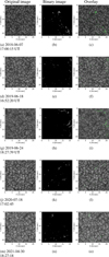 |
Fig. 5 Segmentation results of our trained MBP-TransCNN network. The first column shows the original image of the MBPs. The second column presents a binary image labeled as a MBP. The third column shows the corresponding TiO-band image with MBPs marked in green. |
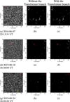 |
Fig. 6 Segmentation results with and without the Transformer branch. The first column corresponds to the input image, the second column displays the segmentation result without the Transformer branch, and the third column shows the segmentation result obtained using the Transformer branch. The red boxes indicate examples where the use of a dual-branch network leads to more precise feature extraction and improved MBP segmentation. The yellow boxes indicate instances where the dual-branch network results in fewer misidentifications of MBPs. |
4.2 Comparative experiment
In this section, we present a comparative analysis of our proposed MBP-TransCNN segmentation network with regard to existing methods for MBP segmentation. We compare our results with the traditional MBP segmentation method proposed by Liu et al. (2018) in Sect. 4.2.1 as well as with the deep learning method proposed by Yang et al. (2019) in Sect. 4.2.2. The runtime and the five evaluation metrics of the segmentation methods proposed by Yang et al. (2019) and by us are presented in Sect. 4.2.3.
We note that the code for the methods of Liu et al. (2018) and Yang et al. (2019) was either not provided or could not be executed. For the method of Liu et al. (2018), we made every effort to replicate it as presented in the paper proposed by Liu et al. (2018). As for the method of Yang et al. (2019), we utilized the Mask RCNN implementation in Wu et al. (2019) and followed the preprocessing steps and network parameter settings outlined in Yang et al. (2019) to ensure a fair and comprehensive comparison.
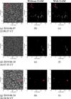 |
Fig. 7 Segmentation results with and without the EAM. The first column corresponds to the input image, the second column displays the segmentation result without the EAM, and the third column shows the segmentation result obtained using the EAM. The red boxes indicate examples where edge features extracted by the EAM algorithm lead to better segmentation results of the MBPs. |
4.2.1 Comparison to traditional methods
In this section, we compare our method with the traditional MBP recognition method of Liu et al. (2018) using ten Big Bear Solar Observatory images in the TiO-band. These images contain MBPs from different time periods and with different shapes and thus presented various challenges to achieving accurate segmentation of the fine structures of the MBPs.
Figure 8 illustrates that the traditional MBP recognition method of Liu et al. (2018) has many misidentifications and that it cannot recognize complete contours of blocky and complex-shaped MBPs. This is mainly because, in traditional methods, the edge gradient of sun granulation is high, and after using Laplacian, the edge of sun granulation is easily misidentified as MBPs. Moreover, traditional methods are sensitive to brightness, and when there are brightness fluctuations, the recognition performance is poor, and they cannot robustly handle various complex situations. In contrast, our proposed MBP-TransCNN method based on powerful CNNs and Transformers can effectively learn the features of MBPs, which significantly reduces the impact of brightness changes and leads to more robust results for complex MBP contours and shapes.
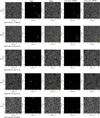 |
Fig. 8 Segmentation results of our method and the method of Liu et al. (2018). The first column shows the input image, and the second and third columns present the segmentation results of our method. The fourth and fifth columns show the segmentation results from the method of Liu et al. (2018). The red boxes and yellow boxes indicate that our method outperforms the method of Liu et al. (2018) significantly. The red boxes indicate that our method produces good segmentation results for complex-shaped MBPs, while the yellow boxes indicate that our method detects fewer misidentified MBPs than the method of Liu et al. (2018). |
Running time of our method and that of Yang et al. (2019).
4.2.2 Comparison to the deep learning Mask RCNN method
We also attempted to reproduce the deep learning Mask RCNN method of Yang et al. (2019). The goal was to compare it to our proposed method using the same annotated MBP dataset for training.
To ensure a fair comparison with the Mask RCNN method proposed by Yang et al. (2019), we followed their preprocessing method. Specifically, we first standardized and normalized all images in our dataset and then applied a 3 × 3 Laplacian kernel convolution filter to enhance the gradient of MBPs. Subsequently, we constructed the dataset by feeding the Laplacian images into the Mask RCNN for training. We adopted the same training parameters as specified in the paper of Yang et al. (2019), such as RPN anchor ratios of 1,2,4,8, and 16; a batch size of ten; and a learning rate of 0.001. In both methods, we used random cropping and rotation for the input dataset. The input image size was set to 640 × 640, and the network was trained for 100 000 iterations until it achieved stable convergence, which required approximately 5 h of training time. We refer to the network trained using the Yang et al. (2019) method as GBP-MRCNN. For our proposed method, we followed the same training strategy, maintaining the image size and number of iterations as mentioned above.
From Fig. 9, it can be seen that the deep learning method of Yang et al. (2019) achieves good results in recognizing point-like MBPs, but for MBPs with complex shapes, such as block-shapes or flower-shapes, the method fails to accurately segment the contours of the MBPs. Thanks to the powerful global feature learning ability of the Transformer, our MBP-TransCNN method shows good robustness regarding complex-shaped MBPs and is less affected by changes in brightness and shape. On the other hand, since the edges of MBPs are not distinct enough, the method of Yang et al. (2019) does not achieve precise edge segmentation of MBPs. In contrast, our proposed EAM method specifically focuses on fine segmentation of MBP edges, ultimately achieving satisfactory segmentation results.
4.2.3 Running time and five evaluation metrics
In this section, we present a comparative analysis of the runtimes and five testing metrics between our proposed method and the method proposed by Yang et al. (2019). Our method directly inputs the original image to predict the MBPs, while the method of Yang et al. (2019) requires preprocessing steps, such as standardization, normalization, and enhancing gradients using the Laplacian convolution kernel, before the image can be used as input in the network to make predictions. Therefore, our inference time does not include any preprocessing time, whereas the inference time of Yang et al. (2019) includes the time for preprocessing. For the time comparison, we used a five-day dataset with the same field of view. The results are presented in Table 3.
Table 3 shows that the average runtime of our proposed method on the five-day dataset is lower than that of the Yang et al. (2019) method (2.06 s). The main reason for this is that the MBPs are embedded in complex backgrounds with significant noise, and the method by Yang et al. (2019) cannot effectively extract the features of the MBPs directly from the original image. As a result, the image needs to be preprocessed to enhance the gradients, which increases the segmentation time.
Table 4 displays the test results of the proposed MBP-TransCNN method and the Yang et al. (2019) GBP-MRCNN method for five time points. The data cover most of the complex MBP scenarios, and the segmentation IoU fluctuates greatly. The Yang et al. (2019) method ranges from 0.234 to 0.413, while our method ranges from a low of 0.715 to a high of 0.880. The average values of precision, recall, F1, PA, and IoU of MBP-TransCNN are 0.976, 0.827, 0.893, 0.999, and 0.808, respectively. In comparison, the Yang et al. (2019) method achieves 0.916, 0.374, 0.526, 0.995, and 0.360 for the same metrics. Our method outperforms the method of Yang et al. (2019) in all the average metrics, particularly in the accuracy metrics calculated pixel by pixel, such as IoU, where our method exhibits greater effectiveness.
4.3 Stability experiment
In order to demonstrate the stability of our segmentation algorithm, we present in Fig. 10 a sequence of 15 consecutive frames showing the segmented MBPs from 2018 June 7. As can be observed from the original frames, the brightness fluctuates slightly over the course of the 15 frames, allowing for a clear view of the evolution of the MBPs. Our segmentation results also exhibit minimal variation and do not introduce significant errors, thus providing an excellent foundation for observing and analyzing the evolution of the MBPs.
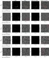 |
Fig. 9 Segmentation results of our method and the method of Yang et al. (2019). The first column shows the input image, and the second and third columns present the segmentation results of our method. The fourth and fifth columns show the segmentation results from the method of Yang et al. (2019). The red boxes show that our method can effectively deal with complex-shaped MBPs, while the method of Yang et al. (2019) misses some detections and produces incomplete segmentation of complete block-shaped MBPs. |
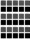 |
Fig. 10 Segmentation results for the time period from 18:55:51 UT to 19:02:51 UT on 2018 June 7. The first, third, and fifth rows display the original images input during this time period, while the second, fourth, and sixth rows display the corresponding segmentation results generated by our proposed MBP-TransCNN method. |
Testing metrics of our method and that of Yang et al. (2019).
5 Conclusions
Magnetic bright points are considered to be good tracers of mag-netic flux tubes on the surface of the solar photosphere. Due to the influence of local convective motions, MBPs often exhibit various morphologies, including simple dot-like shapes, as well as complex shapes, such as chain-like, flower-like, and knee-shaped structures. The dot-like shapes usually represent single, elongated magnetic flux tubes, while the other shapes represent multiple flux tubes located at different positions in concentrated, granular dark regions. The dot-like shapes are mostly isolated MBPs, while the other shapes mostly represent non-isolated MBPs.
With the development of solar observation techniques and astronomical telescopes, the number of solar images has increased, and their resolutions have become higher. In this study, we proposed a deep learning method called MBP-TransCNN, which is based on CNNs and Transformers, to achieve fine structure segmentation of MBP images. By utilizing the strong feature extraction and supervised learning capabilities of CNNs and Transformers, we constructed a dataset of ten original MBP images and used elastic deformation data augmentation to expand the training set to 1000 images for training. The MBP-TransCNN algorithm was trained on a computer equipped with a RTX 3090 (24 GB RAM device), and after 100 000 iterations, it required 9 h of training time until the loss value stabilized and converged. The trained model was tested on the annotated ten-frame MBP dataset captured at different time intervals. The results, as shown in Fig. 5, indicate a good segmentation performance, with an average precision of 0.999, a recall of 0.887, an F1 of 0.920, a PA of 0.963, and a segmentation IoU of 0.854. The experimental results demonstrate that the MBP-TransCNN deep learning method can accurately and rapidly segment the MBP structures in GST observational data.
Our method achieves stable and satisfactory segmentation results for complex and small MBPs. Therefore, our approach can automatically process a large amount of observational data and generate reproducible MBP segmentation results that can facilitate research on solar physics and the solar magnetic field. Our proposed MBP-TransCNN can be readily extended to perform pixel-level segmentation of other types of solar images, a topic that we plan to investigate in future studies.
Acknowledgements
This work was supported by Yunnan Province Ten thousand Talents Program. This work was funded by the National Natural Science Foundation of China (11727805). We gratefully acknowledge the use of data from the Goode Solar Telescope (GST) of the Big Bear Solar Observatory (BBSO). The BBSO operation is supported by US NSF AGS-1821294 grant and New Jersey Institute of Technology. GST operation is partly supported by the Korea Astronomy and Space Science Institute and the Seoul National University.
Appendix A A small machine learning glossary
| Machine Learning Terms | Brief Explanation |
|---|---|
| Encoder | An neural network architecture that transforms input data into a high-dimensional representation, commonly utilized for tasks involving feature extraction and representation learning. |
| CNN (Convolutional Neural Network) | A widely used deep learning model suitable for tasks involving data with grid-like structures, such as images and audio. It utilizes convolutional operations to extract local features from the input data. |
| Transformer | A neural network architecture based on self-attention mechanisms, primarily used for processing sequential data, such as natural language and time series data. It exhibits parallel computation capability and the ability to model long-range dependencies. |
| Hybrid Encoder | A technique that combines different types of encoders to leverage their respective strengths. It often involves the combination of structures like CNN and Transformer to enhance representation learning in tasks involving complex data, such as images. |
| Global Attention | An attention mechanism that considers all positions in a sequence during computation at each position. It aims to capture global semantic information. |
| Feature Fusion | The process in the fields of computer vision and image processing where features from different sources or processing stages are combined to extract richer and more representative information, thereby improving model performance. |
| Global Semantic Information | This refers to the portion of data that encompasses the overall semantic information rather than just local or regional information. |
| Weighted Loss | In the training of neural networks, this is the process of assigning different weights to the loss function for different samples or different parts in order to adjust their influence on the model training. |
| ReLU (Rectified Linear Unit) | A commonly used activation function in neural networks. It is used to introduce non-linearity by setting negative input values to zero and preserving positive input values. |
| Vision Transformer | A neural network model based on the Transformer architecture specifically designed for processing image data. It divides the image into smaller patches and employs Transformers for feature extraction and modeling. |
| Mask RCNN (Mask Region-based Convolutional Neural Network) | A deep learning model that combines object detection and semantic segmentation tasks and is capable of simultaneously detecting the positions of objects in an image and generating precise pixel-level segmentation masks for the objects. |
| Multihead Self-Attention | A mechanism that allows an input sequence to attend to different parts of itself simultaneously using multiple attention heads, enhancing its ability to capture complex relationships and dependencies. |
| Multi-Layer Perceptron (MLP) | A type of feedforward neural network architecture composed of multiple layers of interconnected nodes, or neurons, where each neuron in a layer is connected to every neuron in the subsequent layer, enabling the model to learn complex nonlinear relationships between inputs and outputs. |
References
- Abramenko, V., Yurchyshyn, V., Goode, P., & Kilcik, A. 2010, ApJ, 725, L101 [NASA ADS] [CrossRef] [Google Scholar]
- Anđić, A., Chae, J., Goode, P., et al. 2011, ApJ, 29 [Google Scholar]
- Bai, H. 2022, ArXiv e-prints [arXiv:2210.02635] [Google Scholar]
- Berger, T. E., Schrijver, C. J., Shine, R. A., et al. 1995, ApJ, 454, 531 [NASA ADS] [CrossRef] [Google Scholar]
- Berger, T. E., Löfdahl, M. G., Shine, R. A., et al. 1998, ApJ, 506, 439 [NASA ADS] [CrossRef] [Google Scholar]
- Cao, W., Gorceix, N., Coulter, R., et al. 2010, Astron. Nachr., 331, 636 [Google Scholar]
- Chen, J., Lu, Y., Yu, Q., et al. 2021, ArXiv e-prints [arXiv:2102.04306] [Google Scholar]
- Crockett, P. J., Jess, D. B., Mathioudakis, M., & Keenan, F. 2009, MNRAS, 397, 1852 [CrossRef] [Google Scholar]
- Deng, J., Dong, W., Socher, R., et al. 2009, in 2009 IEEE Conference on Computer Vision and Pattern Recognition, 248 [CrossRef] [Google Scholar]
- De Pontieu, B. 2002, ApJ, 569, 474 [CrossRef] [Google Scholar]
- Dosovitskiy, A., Beyer, L., Kolesnikov, A., et al. 2020, ArXiv e-prints [arXiv:2010.11929] [Google Scholar]
- Dunn, R. B., & Zirker, J. B. 1973, Solar Phys., 33, 281 [NASA ADS] [CrossRef] [Google Scholar]
- Fedun, V., Shelyag, S., & Erdélyi, R. 2010, ApJ, 727, 17 [Google Scholar]
- Feng, S., Ji, K.-F., Deng, H., Wang, F., & Fu, X.-D. 2012, J. Korean Astron. Soc., 45, 167 [NASA ADS] [CrossRef] [Google Scholar]
- Gao, Y., Li, F., Li, B., et al. 2021, Solar Phys., 296, 184 [NASA ADS] [CrossRef] [Google Scholar]
- He, K., Zhang, X., Ren, S., & Sun, J. 2016, in Proceedings of the IEEE Conference on Computer Vision and Pattern Recognition, 770 [Google Scholar]
- He, K., Gkioxari, G., Dollár, P., & Girshick, R. 2017, in Proceedings of the IEEE International Conference on Computer Vision, 2961 [Google Scholar]
- Hofmeister, S. J., Utz, D., Heinemann, S. G., Veronig, A., & Temmer, M. 2019, A&A, 629, A22 [NASA ADS] [CrossRef] [EDP Sciences] [Google Scholar]
- Jess, D. B., Mathioudakis, M., Erdélyi, R., et al. 2009, Science, 323, 1582 [Google Scholar]
- Lin, T.-Y., Goyal, P., Girshick, R., He, K., & Dollár, P. 2020, IEEE Trans. Pattern Anal. Mach. Intell., 42, 318 [CrossRef] [Google Scholar]
- Liu, Y., Xiang, Y., Erdelyi, R., et al. 2018, ApJ, 856, 17 [NASA ADS] [CrossRef] [Google Scholar]
- Long, J., Shelhamer, E., & Darrell, T. 2015, in Proceedings of the IEEE Conference on Computer Vision and Pattern Recognition, 3431 [Google Scholar]
- Magyar, N., Utz, D., Erdélyi, R., & Nakariakov, V. M. 2021, ApJ, 911, 75 [NASA ADS] [CrossRef] [Google Scholar]
- Müller, H.-R., Zank, G. P., & Lipatov, A. S. 2000, J. Geophys. Res., 105, 27419 [CrossRef] [Google Scholar]
- Mumford, S. & Erdélyi, R. 2015, MNRAS, 449, 1679 [NASA ADS] [CrossRef] [Google Scholar]
- Mumford, S., Fedun, V., & Erdélyi, R. 2015, ApJ, 799, 6 [NASA ADS] [CrossRef] [Google Scholar]
- Saavedra, G. B., Utz, D., Domínguez, S. V., et al. 2022, A&A, 657, A79 [NASA ADS] [CrossRef] [EDP Sciences] [Google Scholar]
- Simard, P. Y., Steinkraus, D., Platt, J. C., et al. 2003, Seventh International Conference on Document Analysis and Recognition, 2003. Proceedings Edinburgh, 958 [Google Scholar]
- Utz, D., Hanslmeier, A., Möstl, C., et al. 2009, A&A, 498, 289 [NASA ADS] [CrossRef] [EDP Sciences] [Google Scholar]
- Vigeesh, G., Fedun, V., Hasan, S., & Erdélyi, R. 2012, ApJ, 755, 18 [NASA ADS] [CrossRef] [Google Scholar]
- Wu, Y., Kirillov, A., Massa, F., Lo, W.-Y., & Girshick, R. 2019, https://github.com/facebookresearch/detectron2 [Google Scholar]
- Xiong, J., Yang, Y., Jin, C., et al. 2017, ApJ, 851, 42 [NASA ADS] [CrossRef] [Google Scholar]
- Xu, L., Yang, Y., Yan, Y., et al. 2021, ApJ, 911, 32 [NASA ADS] [CrossRef] [Google Scholar]
- Yang, Y.-F., Lin, J.-B., Feng, S., et al. 2014, Res. Astron. Astrophys., 14, 741 [CrossRef] [Google Scholar]
- Yang, Y., Li, Q., Ji, K., et al. 2016, Solar Phys., 291, 1089 [NASA ADS] [CrossRef] [Google Scholar]
- Yang, Y., Li, X., Bai, X., et al. 2019, ApJ, 887, 129 [NASA ADS] [CrossRef] [Google Scholar]
All Tables
All Figures
|
Fig. 1 Elastic deformation of the image and the result. (a) Original image of the MBP. (b) Binary image labeled MBP. (c) Original image after elastic transformation. (d) Binary image of the same labeled image after the same elastic deformation. |
| In the text | |
|
Fig. 2 Overview of the framework of the proposed MBP-TransCNN. |
| In the text | |
|
Fig. 3 Schematic of the Transformer layer. |
| In the text | |
|
Fig. 4 Schematic diagram of EAM. EAM is designed to excavate marginal features related to small target objects. |
| In the text | |
|
Fig. 5 Segmentation results of our trained MBP-TransCNN network. The first column shows the original image of the MBPs. The second column presents a binary image labeled as a MBP. The third column shows the corresponding TiO-band image with MBPs marked in green. |
| In the text | |
|
Fig. 6 Segmentation results with and without the Transformer branch. The first column corresponds to the input image, the second column displays the segmentation result without the Transformer branch, and the third column shows the segmentation result obtained using the Transformer branch. The red boxes indicate examples where the use of a dual-branch network leads to more precise feature extraction and improved MBP segmentation. The yellow boxes indicate instances where the dual-branch network results in fewer misidentifications of MBPs. |
| In the text | |
|
Fig. 7 Segmentation results with and without the EAM. The first column corresponds to the input image, the second column displays the segmentation result without the EAM, and the third column shows the segmentation result obtained using the EAM. The red boxes indicate examples where edge features extracted by the EAM algorithm lead to better segmentation results of the MBPs. |
| In the text | |
|
Fig. 8 Segmentation results of our method and the method of Liu et al. (2018). The first column shows the input image, and the second and third columns present the segmentation results of our method. The fourth and fifth columns show the segmentation results from the method of Liu et al. (2018). The red boxes and yellow boxes indicate that our method outperforms the method of Liu et al. (2018) significantly. The red boxes indicate that our method produces good segmentation results for complex-shaped MBPs, while the yellow boxes indicate that our method detects fewer misidentified MBPs than the method of Liu et al. (2018). |
| In the text | |
|
Fig. 9 Segmentation results of our method and the method of Yang et al. (2019). The first column shows the input image, and the second and third columns present the segmentation results of our method. The fourth and fifth columns show the segmentation results from the method of Yang et al. (2019). The red boxes show that our method can effectively deal with complex-shaped MBPs, while the method of Yang et al. (2019) misses some detections and produces incomplete segmentation of complete block-shaped MBPs. |
| In the text | |
|
Fig. 10 Segmentation results for the time period from 18:55:51 UT to 19:02:51 UT on 2018 June 7. The first, third, and fifth rows display the original images input during this time period, while the second, fourth, and sixth rows display the corresponding segmentation results generated by our proposed MBP-TransCNN method. |
| In the text | |
Current usage metrics show cumulative count of Article Views (full-text article views including HTML views, PDF and ePub downloads, according to the available data) and Abstracts Views on Vision4Press platform.
Data correspond to usage on the plateform after 2015. The current usage metrics is available 48-96 hours after online publication and is updated daily on week days.
Initial download of the metrics may take a while.