| Issue |
A&A
Volume 677, September 2023
|
|
|---|---|---|
| Article Number | A65 | |
| Number of page(s) | 17 | |
| Section | Atomic, molecular, and nuclear data | |
| DOI | https://doi.org/10.1051/0004-6361/202346518 | |
| Published online | 05 September 2023 | |
Rotational spectrum and interstellar detection of the first torsionally excited state of methylamine★
1
Univ. Lille, CNRS, UMR 8523 – PhLAM – Physique des Lasers Atomes et Molécules,
59000
Lille, France
e-mail: roman.motiyenko@univ-lille.fr
2
Max-Planck-Institut für Radioastronomie,
Auf dem Hügel 69,
53121
Bonn, Germany
3
Université Paris-Cité and Univ. Paris-Est Creteil, CNRS, LISA,
75013
Paris, France
4
Radiospectrometry Department, Institute of Radio Astronomy of NASU,
Mystetstv 4,
61002
Kharkiv, Ukraine
5
Faculty of Chemistry, Adam Mickiewicz University in Poznań,
ul. Uniwersytetu Poznańskiego 8,
61-614
Poznań, Poland
Received:
28
March
2023
Accepted:
14
June
2023
Context. Methylamine (CH3NH2) was first detected in the interstellar medium (ISM) toward Sgr B2 almost 50 years ago by observation of rotational transitions in its torsional ground state. Methylamine exhibits two large-amplitude motions (LAMs), the methyl torsion and amine wagging, which complicate the spectral analysis, especially in excited vibration states. The lack of an accurate model of the two coupled LAMs has also hampered the identification in the ISM of rotational transitions in excited vibrational states.
Aims. The aim of this work is to study the terahertz and microwave rotational spectra of methylamine experimentally and theoretically in order to provide a reliable basis for the detection of its rotational transitions in the first torsionally excited state, υt = 1, in the ISM.
Methods. The terahertz spectrum of methylamine was measured from 150 to 1520 GHz with the Lille fast scan spectrometer. Using a new “hybrid” Hamiltonian model, we were able to analyze the nuclear quadrupole hyperfine structure and to accurately fit the rotational spectrum of the υt = 1 state of methylamine. We used the imaging spectral line survey ReMoCA performed with the Atacama Large Millimeter/submillimeter Array (ALMA) to search for rotational transitions of methylamine in its first torsionally excited state toward the high-mass star forming region Sgr B2(N). The observed spectra are modeled under the assumption of local thermodynamic equilibrium (LTE).
Results. Accurate spectral predictions were obtained for the ground and first excited states of CH3NH2. We report the first interstellar detection of methylamine in the υt = 1 state toward the offset position Sgr B2(N1S) in the hot molecular core Sgr B2(N1). The LTE parameters derived previously from the rotational emission of methylamine in its torsional ground state toward Sgr B2(N1S) yield synthetic spectra of methylamine in the υt = 1 state that are fully consistent with the ALMA spectra and allow us to identify five rotational lines of this state.
Key words: ISM: molecules / methods: laboratory: molecular / submillimeter: ISM / molecular data / line: identification
Full Tables B.1 and B.2 are only available at the CDS via anonymous ftp to cdsarc.cds.unistra.fr (130.79.128.5) or via https://cdsarc.cds.unistra.fr/viz-bin/cat/J/A+A/677/A65
© The Authors 2023
 Open Access article, published by EDP Sciences, under the terms of the Creative Commons Attribution License (https://creativecommons.org/licenses/by/4.0), which permits unrestricted use, distribution, and reproduction in any medium, provided the original work is properly cited.
This article is published in open access under the Subscribe to Open model. Subscribe to A&A to support open access publication.
1 Introduction
Methylamine (CH3NH2) is a seven-atom organic molecule and the simplest primary alkylamine. It is considered to be a possible precursor of the simplest amino acid, glycine, NH2CH2COOH (Holtom et al. 2005). In particular, the radical–radical reaction of CH2NH2 and HOCO in the gas phase, on grain surface, and in bulk ice is considered to be one of the most feasible glycine formation routes (see Joshi & Lee 2022, and references therein). Another recent review (see Aponte et al. 2017, and references therein) provides an analysis of potential synthetic routes of glycine and methylamine from a common set of precursors present in carbonaceous chondrite meteorites, as both molecules have also been detected in multiple extraterrestrial samples (e.g., Pizzarello & Holmes 2009).
Methylamine was first detected in the interstellar medium (ISM) almost 50 years ago by observation of rotational transitions in its torsional ground state toward the high-mass star forming region Sagittarius B2 (Sgr B2) located in the Galactic center region (Kaifu et al. 1974; Fourikis et al. 1974). For a long time, methylamine was only securely detected toward Sgr B2, in particular in its hot molecular cores, Sgr B2(N) and Sgr B2(M) (Belloche et al. 2013; Halfen et al. 2013). With the imaging spectral line survey Re-exploring Molecular Complexity with ALMA (ReMoCA) performed toward Sgr B2(N) with the Atacama Large Millimeter/submillimeter Array (ALMA; Belloche et al. 2019), the abundance of methylamine was found to be 0.07 relative to methanol toward the main hot core of Sgr B2(N) (Kisiel et al. 2022; Motiyenko et al. 2020). Methylamine was also detected in G+0.693−0.27, a shocked region of the Sgr B2 molecular cloud complex not related to the hot cores, with an abundance of 0.2 relative to methanol, which is close to the value derived toward the main hot core of Sgr B2(N) (Zeng et al. 2018; Rodríguez-Almeida et al. 2021)1. A tentative detection for the first time outside the Galactic center region was reported with ALMA in the nearby star forming region Orion KL by Pagani et al. (2017).
Nondetections of methylamine were reported in a number of hot cores by Ligterink et al. (2015) with upper limits to the abundance ratio of methylamine to methanol of between 0.02 and 2, most of them being at a similar level to the ratio measured toward the main hot core of Sgr B2(N). However, a nondetection was also reported toward the low-mass Class 0 protostar IRAS 16293–2422B, where the abundance of methylamine relative to methanol was determined to be lower than 5.3 × 10⁻⁵, which is nearly three orders of magnitude lower than in Sgr B2(N) (Ligterink et al. 2018). This substantial difference departs from the overall good correlation found by Jørgensen et al. (2020) between the abundances of complex organic molecules, that is, carbon-bearing molecules containing at least six atoms (Herbst & van Dishoeck 2009), in IRAS 16293-2422B and the secondary hot core of Sgr B2(N).
Ohishi et al. (2019) detected methylamine with the Nobeyama radio telescope in another hot core, G10.47+0.03. Bøgelund et al. (2019) also managed to detect CH3NH2 with ALMA toward at least one hot core within the molecular cloud complex NGC 63342, with an abundance ratio relative to methanol of about one order of magnitude lower than that found for the main hot core of Sgr B2(N). These detections, along with the detection in Orion KL, suggest that methylamine is more widespread – albeit difficult to detect – in our Galaxy than initially thought. Methylamine has even been detected with the Australia Telescope Compact Array (ATCA) in the disk of a spiral galaxy at a redshift of 0.89 (Muller et al. 2011). The detection was made in absorption against the bright background quasar PKS 1830–211. Muller et al. (2011) derived a methylamine abundance on the order of 0.1–0.2 relative to methanol, which is similar to the ratios measured in the main hot core of Sgr B2(N) and G+0.693−0.027.
On the chemical modeling side, the recent models of gasgrain chemistry in hot molecular cores presented by Garrod et al. (2022) predict that methylamine is predominantly formed in the ice mantles of dust grains at low temperature during the prestellar phase. The ratio of peak gas-phase abundances of methylamine to methanol during the warm-up phase predicted by these models is in the range 0.03−0.04 depending on the warm-up timescale, which agrees within a factor of about two with the ratio reported above for the main hot core of Sgr B2(N). This agreement suggests that the formation of methylamine in Sgr B2 is dominated by radical reactions in the solid phase rather than gas-phase chemistry.
Given the intensities of the υt = 0 transitions of methylamine measured toward Sgr B2(N1S) with the ReMoCA survey and their rotational temperature of ~230 K (Kisiel et al. 2022), we expected the strongest υt = 1 transitions of methylamine to be detectable above the 3σ level in this survey. Detecting such rotational transitions within the first torsionally excited state requires laboratory measurements and a good spectroscopic modeling of their frequencies and intensities.
So far, methylamine has only been detected in its ground torsional state, mainly due to the lack of a complete and precise spectroscopic database in the excited states. In this paper, we derive those parameters for the first excited torsional state of methylamine. The methylamine rotational spectrum has a complex structure due to two coupled large-amplitude motions: the methyl torsion and the amine inversion, or wagging. The ground rotational state of methylamine was successfully analyzed using the effective Hamiltonian approach (high-barrier “tunneling” approach) of Ohashi and Hougen (Ohashi & Hougen 1987). In this approach, each υt torsional state is fitted separately (with its own set of molecular parameters). The analysis yielded an accurate model of the rotational spectrum in the υt= 0 state (Ilyushin et al. 2005; Motiyenko et al. 2014), but showed some limitations with respect to the υt= 1 state. To overcome these limitations, we use a new hybrid model and the BELGI-hybrid code described in Kleiner & Hougen (2015) which takes into account all the torsional states arising from internal rotation of the methyl group of methylamine in a global way (Kleiner & Hougen 2020). The second large-amplitude motion of the NH2 inversion is taken into account within the tunneling approach.
In our first paper on CH3NH2 (Kleiner & Hougen 2020), we used a dataset for υt = 0 and 1 that combines previously published data in the infrared (Ohashi et al. 1987, 1988; Gulaczyk et al. 2017) with data in the microwave spectral range (Motiyenko et al. 2014; Ohashi et al. 1989; Kreglewski & Wlodarczak 1992; Ilyushin et al. 2005; Ilyushin & Lovas 2007), which were fitted using the tunneling formalism from Hougen and Ohashi. We successfully fitted 11880 υt= 1 ← 0 transitions in the far-infrared spectral range, as well as 2288 rotational transitions belonging to the ground torsional state υt= 0 in the microwave spectral range, but we only fitted a limited number (137) of pure rotational transitions belonging to the first excited state υt = 1−1. The aim of this paper is to extend our analysis of the first torsionally excited state of methylamine using the “hybrid” approach.
The paper is divided into five further sections. Section 2 describes the experimental details. Section 3 presents the spectral data used in the present fit. Section 4 describes the Hamiltonian theoretical model and BELGI-hybrid code that we used, including the nuclear quadrupole hyperfine structure and the intensity calculation. Section 5 presents the results of the search for υt = 1 rotational transitions of methylamine in the ISM, and Sect. 6 gives a discussion of some spectroscopic and observational issues connected to our current results. The conclusions of this work are presented in Sect. 7.
2 Experimental details
We performed a new series of measurements of the rotational spectrum of methylamine in the framework of the present study. All the spectra were recorded in absorption mode using the Lille fast-scan hybrid spectrometer (Zakharenko et al. 2015; Motiyenko et al. 2019). The measurements cover the frequency range 150 – 1520 GHz with a few small gaps. We used a 99% pure commercial sample of methylamine purchased from Sigma-Aldrich. The optimal gas pressure in the absorption cell for the best signal-to-noise ratio (S/N) of the recorded spectra was between 30 µbar and 60 µbar, with higher pressures preferred at higher frequencies. Due to partially resolved or unresolved nuclear quadrupole hyperfine structure, the measurement uncertainty is estimated to be around 60 kHz for relatively strong isolated lines and 100 kHz for weak or slightly distorted line shapes, and for the lines measured above 1 THz due to line broadening effects (both Doppler and pressure).
As the main goal of the study is the assignment of excited vibrational states, the spectra were acquired with an increased amplitude resolution. In standard conditions, the spectral amplitude resolution is limited by the resolution of the analog-to-digital converter. In the present study, we used a SR7270 DSP lock-in amplifier, the ADC of which has a resolution of 16 bits. To increase the amplitude resolution, each spectral segment was recorded twice with two gain factors that differed by 20 dB. Lower gain spectra were used to assign the strongest lines, whereas higher gain spectra were particularly useful for the assignment of weak lines in excited torsional states.
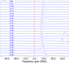 |
Fig. 1 Loomis-Wood diagram centered on predicted frequencies of E1 cQ-type series of transitions of methylamine with |

3 Spectral data
3.1 Microwave, millimeter, and submillimeter data
The assignment of the rotational spectrum of methylamine in excited vibrational states was aided by Loomis-Wood-type diagrams (Loomis & Wood 1928). These diagrams allow the accurate assignment of broadband spectra, especially at the initial stage of analysis when predicted transition frequencies may be significantly different from observed ones. The technique consists in superposing portions of spectra centered on predicted frequencies of a particular series of transitions where only one quantum number is varied and the rest are kept constant. In this case, the shifts of the observed lines with respect to the predicted ones exhibit a smooth (typically polynomial) behavior as a function of the varied quantum number and can be easily located on the diagram. An example of a Loomis-Wood plot for a series of υt = 1−1 rotational transitions is shown in Fig. 1. This latter was built using the predicted frequencies from our previous study (Kleiner & Hougen 2020). Even if the lines are shifted with respect to predictions by 15 to 20 MHz, the smooth variation allows easy identification. After the series was included in the fit, and after the refinement of the Hamiltonian parameters, the newly predicted frequencies almost coincide with the observed ones. In this case, all experimental lines would be vertically aligned on the new diagram. To build Loomis-Wood plots, we used home-made software for spectral analysis, which is available from the corresponding author upon request.
In the present study, using the new spectra records, the dataset for the ground torsional state υt = 0−0 was increased to 2790 microwave, millimeter and submillimeter transitions, compared to the published 2400 transitions up to J = 40 from the supplementary material from Motiyenko et al. (2014) and compared to our previous fit of 2288 transitions from Kleiner & Hougen (2020). For the first excited state, about 212 microwave lines existed in the literature (Ohashi et al. 1987, Ohashi et al. 1988; Gulaczyk et al. 2017) and in our previous paper we only fitted 137 of them (Kleiner & Hougen 2020). In the present work, we were able to assign and fit 2921 new υt = 1−1 rotational transitions. These were combined with previously assigned υt = 1−1 lines in the frequency range 49–149 GHz (Motiyenko, priv. comm.). These assignments were done using the spectrum records obtained for methylamine by Ilyushin et al. (2005). In addition, 40 υt = 2−2 rotational transitions were also newly assigned and fitted. We also replaced 3 lines from Kreglewski & Wlodarczak (1992) and 132 lines from Ohashi et al. (1989) with our more accurate measurements.
As in our previous paper, the frequency measurement uncertainties of microwave transitions ranged between 20 kHz, 50 kHz, 60 kHz, 100 kHz, 200 kHz, and 500 kHz depending on the measurement source. The hyper fine structure was removed for most of those lines in the literature, but for some of them this was done only by visual inspection, and so they were given a weight of 500 kHz, whereas the hyperfine splittings for the lines from Motiyenko et al. (2014) were removed properly, and so they were given weights from 20 to 200 kHz (see Sect. 2 of Kleiner & Hougen 2020).
3.2 Far-infrared data
The number of transitions in the far-infrared fundamental band υt = 1 ← 0 was kept about the same (11643) as in our previous paper (11880) with J up to 40 and K up to 17. In the present fit, we added 6155 transitions belonging to the hot band υt = 2 ← 1 and 5253 transitions belonging to the overtone υt = 2 ← 0 from (Gulaczyk et al. 2018; Gulaczyk & Kreglewski 2020). We decided to include neither the previously published ground state υt = 0 combination differences (GSCDs) – as their large number tends to decrease the impact of the more accurate microwave transitions, thus causing the parameters to drift – nor the pure rotational transitions υt = 0−0, υt = 1−1 or υt = 2−2, which were initially measured in the far-infrared range, as for a number of them our remeasurements in high-resolution THz spectra obtained in this study showed discrepancies in the measured frequencies of up to 30 MHz, which is much higher than the microwave measurement accuracy.
3.3 Hyperfine structure analysis
In methylamine, the interaction of the 14N electric quadrupolar moment with the molecular field gradient results in the hyperfine structure of the rotational spectrum. The interaction couples the nuclear spin I to the molecular rotational angular momentum J to form a resultant total angular momentum vector F. As the nuclear spin of 14N is I = 1, each rotational level of methylamine is split into three hyperfine sublevels: F = J + 1, F = J, and F = J−1. The transitions between hyperfine levels obey the selection rules ∆F = 0, ±1 and can give rise to a complex hyperfine structure for low- J rotational transitions. With increasing J, only hyperfine transitions with ∆F = ∆J selection rule are usually observed, as their sum of relative intensities represents more than 99% of the total intensity of the hyperfine components for a given rotational transition. Therefore, the hyperfine structure for high- J transitions of methylamine is usually represented by three components.
Due to Doppler-limited spectral resolution, the hyperfine structure in the spectrum of methylamine has only been partially resolved for a limited number of rotational transitions. A resolved pattern of the hyperfine structure was observed as a doublet with an intensity ratio of 2:1. The stronger doublet component contains unresolved transitions with F′ = J′ + 1 ← F′ = J + 1 and F′ = J′ – 1 ← F = J – 1 selection rules, whereas the weaker doublet component corresponds to the F′ = J′ ← F = J transition. An example of partially resolved hyperfine structure for a υt = 1–1 rotational transition of methylamine is shown in Fig. 2.
Each hyperfine transition frequency may be expressed as
 (1)
(1)
where frot is the hyperfine-free central frequency and Ehf denotes the addition to the energy due to hyperfine coupling. Ehf may be expressed in terms of rotational angular momentum operators and nuclear quadrupole coupling tensor components χij, i, j = a, b, c as (Ilyushin et al. 2005):
![$\matrix{ {{E_{{\rm{hf}}}}\left( {I,J,F} \right) = \left[ {{1 \over 2}{\chi _ + }\left\langle {J_b^2 + J_c^2 - 2J_a^2} \right\rangle - {1 \over 2}{\chi _ - }\left\langle {J_b^2 - J_c^2} \right\rangle } \right.} \hfill \cr {\left. {\,\,\,\,\,\,\,\,\,\,\,\,\,\,\,\,\,\,\,\,\,\,\,\,\,\,\,\,\,\, + {\chi _{ab}}\left\langle {{J_a}{J_b} + {J_b}{J_a}} \right\rangle } \right]{{2f\left( {I,J,F} \right)} \mathord{\left/ {\vphantom {{2f\left( {I,J,F} \right)} {J\left( {J + 1} \right)}}} \right. \kern-\nulldelimiterspace} {J\left( {J + 1} \right)}}} \hfill \cr } $](/articles/aa/full_html/2023/09/aa46518-23/aa46518-23-eq3.png) (2)
(2)
where χ+ = −χaa, χ− = χcc − χbb and f(I, J, F) is the Casimir function (Gordy & Cook 1984).
Equations (1) and (2) were used to obtain hyperfine-free rotational transition frequencies frot for the global fit. We used a perturbation approach similar to that used for acetamide, a Cs molecule with one methyl internal rotor large-amplitude motion, and one nitrogen quadrupole nucleus (see Eq. (1) of Suenram et al. 2001). The same approach was also used in the analysis of the ground-state rotational spectrum of 12C–methylamine (Ilyushin et al. 2005; Motiyenko et al. 2014) and 13C–methylamine (Motiyenko et al. 2016). Using the BELGI-hybrid code, we obtained the rotation-torsion eigenvalues and eigenvectors from the usual two-step diagonalization of the Hamiltonian HWTR, as described in Sect. 4. The global fitting BELGI-hybrid program was modified to output expectation values of 〈Ja〉2, 〈Jb〉2, 〈Jc〉2, and 〈JaJb + JbJa〉 in the rho axis system (a, b, c). To obtain hyperfine-free rotational transition frequencies, each hyperfine component was fitted to Eq. (1). The linear least-squares Gauss-Newton algorithm was applied using a dedicated Python code. In the present study, we assigned 324 partially resolved hyperfine components of υt = 1–1 rotational transitions. These were fitted together with 1132 υt = 0–0 components from this and previous studies (Ilyushin et al. 2005; Motiyenko et al. 2014) to yield 653 hyperfine-free rotational transition frequencies and two hyperfine constants χ+ and χ−, the values of which are given in Table 1. As a point of comparison, the last column of Table 1 provides the corresponding values obtained using high-barrier tunneling Hamiltonian expectation values. As can be seen from Table 1, the χ+ values match well, whereas the χ− values are outside the confidence intervals of both studies. This significant difference in the χ− parameter probably arises from the different Hamiltonians used for obtaining expectation values of the necessary rotational operators. In this connection, it is interesting to note that our current value for χ− = 6.4058(85) MHz is in much better agreement with χ− = 6.3746(81) MHz obtained by Kreglewski et al. (1992), which supports our hypothesis that the difference with our previous result is caused by the difference in the Hamiltonian models used.
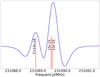 |
Fig. 2 Partially resolved hyperflne structure of the υt = 1–1 141,13–140,14 E1 transition of methylamine. The stick spectrum shows the calculated positions of hyperflne components. |
14N nuclear quadrupole coupling parameters for methylamine
4 Theoretical model and analysis
The theoretical Hamiltonian model used in our fit is the so-called hybrid Hamiltonian, which allows us to deal with the two coupled large-amplitude motions present in methylamine, namely the internal rotation of the methyl group CH3 and the back-and-forth oscillatory inversion motion, or wagging, of the amine group NH2. This approach has been tested in the ground torsional state of methyl-malonaldehyde (Kleiner & Hougen 2015), and also in our previous study of the ground and first excited state of methylamine (Kleiner & Hougen 2020).
As the hybrid model and the BELGI-hybrid code have been presented in detail elsewhere (Kleiner & Hougen 2015, 2020), here we only give a short summary of the approach. In the hybrid Hamiltonian, we mix two methods to deal with the coupling of two large-amplitude motions. The first method treats the internal rotation of the CH3 group in a similar way to the method presented in the series of BELGI programs (Kleiner et al. 1992; Kleiner 2010). Those “BELGI”-type terms contain an explicit form for the potential barrier hindering the methyl internal rotation or torsion. For the internal rotation of the CH3 group, the rotation–torsion Hamiltonian has the form:
 (3)
(3)
where F is the internal rotation constant, Pα is the internal rotation angular momentum, ρ is the coupling constant between internal and global rotation, Jx, Jy, and Jz are angular momentum projections along x, y, and z molecular axes, and V(α) is the potential internal rotation barrier described as a Fourier series:
 (4)
(4)
The second method treats the back-and-forth (wagging) motion of the amino group NH2 using the tunneling approach as described by Ohashi & Hougen (1987). Those tunneling-type terms, which contain matrix elements associated with tunneling between the two positions of the amino group, do not contain any explicit form for the double-well tunneling potential. Instead H = T + V for the wagging motion is replaced with one tunneling splitting parameter plus higher-order torsion-rotation corrections.
Here, we used a two-step diagonalization procedure similar to the one used in the one-top BELGI code (Kleiner et al. 1992; Kleiner 2010). In the first step, we diagonalize the torsion-K-rotation part of the matrix associated with the two first terms of the Hamiltonian given in Eq. (3). We separate the nonde-generate torsional-wagging-rotational (twr) states (of symmetry species twrA1 ⊕ twrA2 ⊕ twrB1 ⊕ twrB2) from the set of doubly degenerate states (of species twrE1 ⊕ twrE2) using the σ = 0 and σ = +1 characters associated with irreducible representations of the permutation-inversion G12 group. We then separately diagonalize the Hamiltonian matrix for each of those two sets.
This torsion-wagging-rotational hybrid Hamiltonian matrix Htwr is partitioned into four square submatrices, as shown in Eq. (1) of Kleiner & Hougen (2020), with blocks noted by L(eft)L(eft), L(eft)R(ight), RL, and RR:
![$\left[ H \right] = \left[ {\matrix{ {{\rm{LL}}} & {{\rm{LR}}} \cr {{\rm{RL}}} & {{\rm{RR}}} \cr } } \right],$](/articles/aa/full_html/2023/09/aa46518-23/aa46518-23-eq6.png) (5)
(5)
where HRR corresponds to the torsion-rotation Hamiltonian, which is identical to that used in the BELGI series of codes for the one-top molecules, where the amino group NH2 of the methylamine molecule is locked in one of its two symmetrically equivalent equilibrium inversion positions and is localized in a well on the positive side of the γ axis, where γ designates the inversion or wagging coordinate. HLL represents the BELGI matrix, which corresponds to a methylamine molecule with the amino group locked in the other of the two symmetrically equivalent equilibrium inversion positions and localized in the negative side of the γ axis. HRL and HLR contain matrix elements that describe the amino group tunneling from the positive region of γ to the negative region, or vice versa; that is, they describe inversion motion.
Overview of a fit of 28 802 transitions of methylamine with J ≤ 40, K ≤ 17, using 79 parameters floated to give a weighted standard deviation of 1.53.
4.1 Fit with the hybrid formalism
The BELGI-hybrid code globally fits a large microwave, millimeter, and submillimeter dataset for 2790 υt = 0–0, 2921 υt = 1–1, and 40 υt = 2 – 2 pure rotational transitions, as well as the far-infrared dataset involving 11643 υt = 1 ← 0, 6155 υt = 2 ← 1, and 5253 υt = 2 ← 0 transitions up to J = 40.
As can be seen from Table 2, we achieve a global unitless standard deviation of 1.53 for 28802 transitions. The quality of the fit is satisfactory, although not completely within experimental uncertainty for the microwave transitions. The upper part of the table presents transitions grouped by their torsional υt quantum numbers (and spectral range) and/or symmetry species. The lower part of the table shows root-mean-squared deviations grouped by assigned measurement uncertainty.
The 79 floated molecular parameters (plus eight additional parameters, which were fixed at values from previous fits, such as F, V9, DK, WCPG (which multiplies the PγJy operator), and some higher order K dependent parameters) are listed in Table A.1 and compared to the 74 floated and two fixed parameters in the previous work, where we fitted a total of 15081 transitions (Kleiner & Hougen 2020). The increase in the number of parameters is very reasonable considering that the number of lines increased by almost a factor of two. As detailed in Kleiner & Hougen (2020), the first column of Table A.1, labeled ntrw, contains four indices describing the order of the term with n = t + r + w, where t and r are the traditional torsional and rotational orders and w is the amino wagging order (see Kleiner & Hougen 2020 for details). The second column gives the name of the molecular parameter as used in the BELGI-hybrid code and the operator that it multiplies. These operators must all be: (i) Hermitian, (ii) of species A1 in the permutation-inversion group G12 (Kleiner & Hougen 2015), and (iii) invariant to time reversal. The third column gives numerical values for the molecular parameters obtained from the previous fit (Kleiner & Hougen 2020), and the fourth column gives the values of the parameters as obtained from the present fit described in Table 2, together with their standard errors. As already mentioned in Kleiner & Hougen (2020), we note that a factor of γ was omitted in three operators of Table 5 of Kleiner & Hougen (2015), namely those multiplied by the coefficients DAB, ODAB, and ODELTA in that table. The correct operators are those given in Table A.1 here, where we also change the name of the ODELTA parameter to AXGK.
Compared to our previous fit, the variation of the second-order term in the potential (V6) is relatively large, showing the influence of the υt = 1 and 2 excited states in determining the potential terms in the Fourier expansion. We also noticed that a number of low-order parameters have changed sign (such as V6, AXG, and DAB which multiply  , γPα Jx term and γ{Jx, Jz} respectively).
Compared to the previous tunneling fits of the literature, here a large reduction in parameters is obtained in our global fit, because the 55 + 88 = 143 tunneling parameters used in the final fit of Gulaczyk & Kreglewski (2020) are reduced by almost a factor of 1.6 to 79 (+8 fixed parameters) in Table A.1. For the far-infrared data, our rms deviations for the fundamental band υt = 1 ← 0, the hot band υt = 2 ← 1, and the overtone υt = 2 ← 0 are 0.00015 cm−1 for 11643 lines, 0.00063 cm−1 for 6155 lines, and 0.00064 cm−1 for 5253 lines compared to the rms of 0.00058 cm−1 for 12237 lines, 0.00209 cm−1 for 6609 lines, and 0.00197 cm−1 for 7735 lines obtained in Gulaczyk & Kreglewski (2020) for the same bands, respectively. This comparison is not totally fair because the number of transitions fitted in Gulaczyk & Kreglewski (2020) is not the same as ours; in their study they fit up to J = 50. In the present work, because of the size of the matrix that we need to take into consideration in our global approach and the computer time required subsequently, we decided to fit only up to J = 40.
In the microwave spectral range, the rms we obtained for the fit of the ground torsional υt = 0–0 state is higher (154 kHz) than the rms obtained by the tunneling approach (102 kHz), but we included 236 more lines in our fit (2790 lines instead of 2554 lines) than in Gulaczyk & Kreglewski (2020). For the first excited state υt = 1–1, we obtained a rms of 218 kHz for 2921 lines. In Gulaczyk & Kreglewski (2020), only 214 transitions were available at that time and these authors fitted them with a rms of 183 kHz. Finally, our υt = 2–2 data fit with a rms of 289 kHz.
In a general way, and this was also noticed in our previous paper (Kleiner & Hougen 2020), poorly fitted lines belong to high J and/or high K transitions and this tendency is also visible in the microwave spectral range. A number of transitions υt = 1 – 1 with K = 0 and 1 in the A and B nondegenerate species did not fit either within experimental accuracy, and large observed-calculated values of up to 1 or 2 MHz are observed. The energy levels of those transitions were shown by Ohashi et al. (1989, see their Figs. 1 and 2) to contribute to an avoided crossing in the case of the B species and to an unavoided crossing for the A species series. We used several Hamiltonian terms with matrix elements connecting energy levels differing by ∆K = ±1 to take into account this perturbation, such as DAB, AXG, DAC (see Table A.1) and so on, but we did not succeed in decreasing the observed-calculated values for those lines with K = 0 and 1 and we finally omitted them in the fit.
The lists of rotational and rovibrational transitions of methylamine are presented in Tables B.1 and B.2 and are available at the CDS3. In the first ten columns of both tables, the quantum numbers for each spectral line are given: υt, J, Ka, Kc, and symmetry label Γ. In the subsequent four columns, we provide the observed transition frequencies, measurement uncertainties, residuals from the fit, and a binary flag indicating whether the transition was included in the final fit. The last column of Table B.1 contains a reference from which the measurements were obtained. The last column of Table B.2 contains an optional flag “L” for υt = 2 ← 1 and υt = 2 ← 0 transitions of A1, A2, B1, and B2 symmetries. The flag indicates that the Ka = 2 and Ka = 4 labels are reversed compared to the labels from Gulaczyk & Kreglewski (2020). This difference in the labeling occurs during the procedure of assignment of the Ka quantum number after the diagonalization of the Hamiltonian matrix and reveals the mixing of the eigenfunctions.
4.2 Intensity calculation
The BELGI-hybrid code was modified to provide the line strength calculations for methylamine transitions. The line strength (S) of the torsion-rotation transition between the level L′ containing all (2 J′ + 1) M′ components and the level L containing all (2 J + 1) M components is given by the formula (Ilyushin & Lovas 2007):
 (6)
(6)
where |K, υt, σ, w〉 and | J, K, M〉 are the torsion-rotation-inversion and symmetric rotor basis functions used to set up the waggingtorsion-rotation Hamiltonian matrix for the second diagonalization step; the coefficients  are the eigenvectors coefficients obtained after diagonalization of the waggingtorsion-rotation Hamiltonian matrix; the ΦZg represents direction cosines, and µg is the electric dipole moment along the molecular-fixed g = x,y, z axis. The electric dipole moment is a function of the methyl torsion angle α and of the amino umbrella γ coordinate (Ilyushin & Lovas 2007). The torsional dependence of µg is given as a Fourier expansion in the torsional angle (see Eq. (19) of Hougen et al. 1994). For the present work, we are concerned with the intensities of pure rotational transitions and so we neglect the cosine and sine dependence of the dipole moment components, and keep only the leading (independent of α) terms. We also neglected the tunneling contributions in γ of the dipole moments, as was also done in Ilyushin & Lovas (2007). For methylamine, the nonzero value of the dipole moment components are µa (µz) and µc (µx ± iµy).
In the Principal Axis Method (PAM), the dipole moment components are measured using Stark effect measurements by Lide (1957), and are then corrected by Takagi & Kojima (1973) with µa = −0.307 D and µc = 1.258 D. In the Rho Axis Method (RAM), those values need to be transformed using Eq. (20) of Kleiner (2010), but since for methylamine the angle between PAM and RAM is very small, the values we used for the dipole moments in this system, namely µa = −0.226 D and µc = 1.275 D, are very close to the PAM ones.
As the hyperfine splittings for methylamine can reach up to a few MHz and are essential in correctly fitting the astronomical spectra, we also calculate the relative intensities of the quadrupole hyperfine components using the formula given by Townes & Schawlow (1955). We multiply the µ2S of each rotational transition by the relative intensity of the quadrupole component. For the intensity calculation we also had to take into account the nuclear spin statistical weight (Wst), which is equal to 1 for A1, A2, and E2 species and to 3 for B1, B2, and E1.
The calculated υt = 1–1 rotational spectrum of methylamine is available at the Lille Spectroscopic Database4 (LSD) in two versions: (1) pure rotational transition frequencies, and (2) a rotational spectrum, taking the nuclear hyperfine structure into account. The spectra may be generated with different line “intensity” units: line strength (D2), Einstein Aij coefficients (s−1), and absorption cross-sections (nm2MHz/molecule). For the latter, the rotational partition function calculated from first principles by Motiyenko et al. (2014) is used. We also note that although the “hybrid” global model used in the present study predicts both υt = 0–0 and υt = 1–1 rotational transitions, in the LSD, we decided to keep the spectral predictions calculated by Motiyenko et al. (2014) as the entries for υt = 0–0 spectra. We did this for two reasons. First, the effective high-barrier tunneling Hamiltonian model from Motiyenko et al. (2014) covers the wider range of rotational quantum numbers up to J ≤ 50, whereas present hybrid model fits rotational levels only up J ≤ 40 (this reduction in the upper value of J is caused by the necessity to keep the computation time within reasonable limits in the case of the hybrid approach because it deals with a much larger basis set than high-barrier tunneling Hamiltonian). Second, we believe that for the υt = 0–0 transitions, high-barrier tunneling formalism provides predictions of slightly better accuracy, as evidenced by the better rms and weighted rms deviations achieved for υt = 0–0 in Motiyenko et al. (2014) in comparison with our current result with the hybrid approach. This is due to the fact that separate state models of the high-barrier tunneling approach do not need to accommodate torsion–rotation and intervibrational perturbations from higher excited states in methylamine. However, this advantage of the high barrier tunneling formalism becomes a disadvantage when we need to deal with the first excited torsional state, where the hybrid approach indeed shows much better results. Therefore, at present, we believe that it is better to use predictions based on the high-barrier tunneling Hamiltonian of Motiyenko et al. (2014) for υt = 0–0 transitions and predictions based on the current hybrid approach for υt = 1–1 transitions.
To illustrate the quality of the rotational transitions of methylamine in the ground and first excited torsional states calculated in this study, we compare an experimental (in blue) and a modeled (in red) spectrum around 1.38 THz in Fig. 3; here, we also show individual contributions of υt = 0−0 and υt = 1−1 transitions. Overall, the agreement in terms of frequency and relative intensity is good. We also note that, in this frequency region, the great majority of strong lines refer to υt = 0−0 and υt = 1−1 transitions.
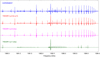 |
Fig. 3 Observed (in blue) and predicted (in red) υt = 0–0 and υt = 1–1 rotational spectrum of methylamine around 1.38 THz. The individual contributions of υt = 0–0 and υt = 1–1 transitions are shown in magenta and green, respectively. Regular series of lines refer to cQ-type transitions with Ka = 9 ← 8 and symmetry selection rules: E1 ← E1 for υt = 0–0, and E1 ← E1 (stronger) and E2 ← E2 (weaker) for υt = 1–1. |
Parameters of our best-fit LTE model of methylamine (with hyperfine structure) toward Sgr B2(NIS).
5 Interstellar detection of methylamine in its first torsionally excited state
5.1 Observations
The imaging spectral line survey Reexploring Molecular Complexity with ALMA (ReMoCA) targeted the high-mass star forming protocluster Sgr B2(N) with ALMA. We used this survey to carry out an interstellar search for methylamine in its first torsionally excited state. The main features of the survey are summarized below. More details about the observations and data reduction can be found in Belloche et al. (2019). The phase center is located at the equatorial position (α,δ)J2000=(17h47m19s.87, −28º22′16″.0), which is halfway between the two hot molecular cores Sgr B2(N1) and Sgr B2(N2). The survey covers the frequency range from 84.1 GHz to 114.4 GHz at a spectral resolution of 488 kHz (1.7 to 1.3 km s−1). This coverage was obtained with five different frequency tunings. The observations achieved a sensitivity per spectral channel ranging between 0.35 mJy beam−1 and 1.1 mJy beam−1 (rms) depending on the setup, with a median value of 0.8 mJy beam−1. The angular resolution (half-power beam width, HPBW) varies between ~0.3″ and ~0.8″ with a median value of 0.6″ that corresponds to ~4900 au at the distance of Sgr B2 (8.2 kpc, Reid et al. 2019). Here, we used the slightly improved version of the data reduction that one of us described in Melosso et al. (2020).
As in Belloche et al. (2019), we analyzed the spectrum obtained toward the position Sgr B2(N1S) at (α,δ)J2000=(17h47m19s.870, −28º22′19.″48), which is offset by about 1″ to the south of the main hot core Sgr B2(N1). This position was chosen for its lower continuum opacity compared to the peak of the hot core. We compared the observed spectrum to synthetic spectra computed under the assumption of local thermodynamic equilibrium (LTE) with the astronomical software Weeds (Maret et al. 2011). This assumption is justified by the high densities of the regions where hot-core emission is detected in Sgr B2(N) (> 1 × 107 cm−3, see Bonfand et al. 2019).
The software takes the angular resolution of the observations and the optical depth of the rotational transitions into account. We derived a best-fit synthetic spectrum for each molecule separately, and then added together the contributions of all identified molecules. Each species was modeled with a set of five parameters: size of the emitting region (θs), column density (N), temperature (Trot), line width (ΔV), and velocity offset (Voff) with respect to the assumed systemic velocity of the source, Vsys = 62 km s−1. The line width and velocity offset are obtained directly from the well-detected and uncontaminated lines. The emission of complex organic molecules is extended over several arcseconds around Sgr B2(N1) (see Busch et al. 2022). For the LTE modeling, we assumed an emission size of 2″, as in Belloche et al. (2019), which is much larger than the beam, meaning that the derived column densities do not depend on the exact value of this size parameter.
5.2 Detection of CH3NH2 in its first torsionally excited state
One of us reported the detection of methylamine in its torsional ground state toward Sgr B2(N1S) in Kisiel et al. (2022; see their Fig. A.5). The analysis presented in this latter study used the spectroscopic entry 31008 (version 1) available in the Jet Propulsion Laboratory (JPL) spectroscopic database (Pickett et al. 1998), which is based on the combined fit by Ilyushin et al. (2005). This entry does not account for the hyperfine structure of methylamine. However, we found that the spectral broadening due to the hyperfine structure is not negligible for some methylamine lines given the typical line width of 5 km s−1 (about 1.7 MHz) toward Sgr B2(N1S). Therefore, here we used the spectroscopic entry 31802 (version 2021.08) of the LSD, which is based on Motiyenko et al. (2014) and accounts for the hyperfine structure.
The LTE synthetic spectrum computed with the LSD entry using the same LTE parameters as those reported in Table 3 of Kisiel et al. (2022) is compared to the ReMoCA spectrum of Sgr B2(N1S) in Fig. C.1. These LTE parameters are listed in Table 3. A detailed comparison of Fig. A.1 to Fig. A.5 of Kisiel et al. (2022) shows that the hyperfine structure does indeed broaden several lines of methylamine and in turn reduces their peak temperature compared to the previous study, where the hyperfine structure was not accounted for (see, e.g., the lines at 84.215, 86.075, or 95.146 GHz). As a result, several lines that were counted as detected in Table 3 of Kisiel et al. (2022) are now below the threshold considered here to count a line as firmly detected. The adopted threshold depends on the degree of contamination of the line, but it roughly corresponds to two-thirds of the peak of the observed line. To count a given line as detected, we also require that there be a clear peak in the observed spectrum at the frequency of this line, and that the peaks of both the synthetic and observed lines be above three times the rms noise level (dotted lines in the figures). With these criteria, we count 10 lines of methylamine in its torsional ground state as detected in Fig. C.1 while 15 were counted in the previous study that ignored the hyperflne structure of methylamine. The ten detected ground-state lines of methylamine are marked with a green star in Fig. C.1.
We computed an LTE synthetic spectrum of the rotational transitions of methylamine in its first torsionally excited state using the spectroscopic predictions obtained in Sect. 4 and assuming the same LTE parameters as for the torsional ground state. This synthetic spectrum is a good match to the ReMoCA spectrum of Sgr B2(N1S) (see Fig. 4). Many transitions are contaminated by emission from other molecules, but five lines of CH3NH2 υt = 1 are strong enough and sufficiently uncontaminated to be counted as detected. They are highlighted with a green star in Fig. 4. One comment should be made concerning the υt = 1 line of methylamine at 86657 MHz. The two strong transitions on each side of this line are from ethylene glycol (CH2OH)2. As can be seen in Fig. 4, the LTE model displayed in blue, which includes the contribution of all identified molecules, slightly overestimates the widths of these ethylene glycol lines in this frequency range, which artificially increases the contamination of the methylamine line that lies in between. This is why we still consider this line of methylamine as being sufficiently uncontaminated.
We produced a population diagram that includes transitions from both torsional states (Fig. 5). After correction for the optical depth of the lines and subtraction of the contamination from other molecules included in our full model (i.e., the difference between the blue and red spectra in Figs. C.1 and 4), the observed data points are roughly distributed along a straight line, which indicates that the emission of methylamine in both torsional states can be described by a single temperature component. A fit to the population diagram yields a rotational temperature of 222 ± 8 K, as reported in Table 4. The temperature that we assumed for the LTE synthetic spectra (see Table 3) is consistent with the temperature derived from the population diagram within 1σ. The partition function of both the υ = 0 and υt = 1 spectroscopic entries includes only the rotational part. The column density derived in Table 3 was corrected to account for the vibrational part of the partition function. This correction was computed in the harmonic approximation using the vibrational energies of methylamine provided by Shimanouchi (1972) and Gulaczyk & Kręglewski (2020).
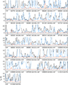 |
Fig. 4 Selection of rotational transitions of methylamine CH3NH2 in its first torsionally excited state covered by the ReMoCA survey. The LTE synthetic spectrum of CH3NH2 υt = 1 is displayed in red and overlaid on the observed spectrum of Sgr B2(N1S) shown in black. The blue synthetic spectrum contains the contributions of all molecules identified in our survey so far, including the contribution of the species shown in red. The values written below each panel correspond from left to right to the half-power beam width, the central frequency in MHz, the width in MHz of each panel in parentheses, and the continuum level in K of the baseline-subtracted spectra in brackets. The y-axis is labeled in brightness temperature units (K). The dotted line indicates the 3σ noise level. The green stars highlight the lines of methylamine in its first torsionally excited state that are not excessively contaminated by emission from other species and are counted as detected lines in Table 3. |
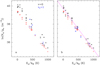 |
Fig. 5 Population diagram of CH3NH2 toward Sgr B2(N1S). The observed data points are shown in black for υ = 0 and in blue for υt = 1 while the synthetic populations are shown in red. No correction is applied in panel a. In panel b, the optical depth correction has been applied to both the observed and synthetic populations and the contamination by all other species included in the full model has been subtracted from the observed data points. The purple line is a linear fit to the observed populations (in linear-logarithmic space). |
Rotational temperature of methylamine derived from its population diagram toward Sgr B2(N1S).
6 Discussion
It is evident that we came up against problems in current analysis that prevented us from achieving a fit within the experimental error for the available dataset. Indeed, as seen from Table 2, even for the torsional ground state, the weighted rms deviation for the microwave data is 2.38. The fact that we get greater rms deviation for the ground state in comparison with the previous fit with the tunneling approach is not surprising. This is because in the present study, we worked with a semi-global approach, which fits the data belonging to a number of torsional states with one set of parameters, and therefore the problems with fitting excited torsional states may also diminish the quality of fitting for the ground state. On the one hand, we are not able to rule out a situation where our current fit corresponds to some local minimum in vicinity of the global minimum in the functional space of Hamiltonian parameters. Indeed, here we deal with the two large-amplitude vibrational motions, which produce a rather complicated landscape in the Hamiltonian parameter space. The fact that a number of low-order parameters (such as V6, AXG, DAB) have changed sign in comparison with our first methylamine study using the hybrid approach (Kleiner & Hougen 2020) shows that, at least with respect to our previous study, we changed our position in the Hamiltonian parameter space quite significantly and therefore we could still be out of a global minimum with our fit. Further extension of the analysis to the second torsionally excited state may provide necessary information for improving the situation with the global versus local minimum by putting additional constraints on the Hamiltonian parameter set. On the other hand, this problem might be circumvented simply by finding an optimal set of high-order parameters in our Hamiltonian model that allow us to take into account all peculiarities of the energy level structure of the excited torsional states. Here, the fact that poorly fitted lines belong to high J and/or high K transitions – as mentioned above – may be considered as an argument in favor of this explanation. Although our search for the high-order Hamiltonian terms that could help to improve the situation was quite extensive, it was not exhaustive, because this search is very time consuming in view of the complexity of the Hamiltonian parameter space in the case of two coupled, large-amplitude motions.
A further possible explanation for the remaining problems with fitting the available dataset is the strong influence of intervibrational interactions arising from low-lying nontorsion vibrations in the molecule. In methylamine, the third excited torsional state is already close in energy to the NH2 wagging mode (see e.g., Fig. 2 of Gulaczyk et al. 2017) and strong Fermi and Coriolis-type resonances have been reported for this state (Gulaczyk et al. 2010). Therefore, it is quite probable that these perturbations propagate down through numerous intertorsional interactions and affect the energy level structure of the lower torsional states. Our current model is not capable of explicitly taking these intervibrational interactions into account since the tunneling part of the hybrid approach represents only a separate wagging state (in our current case, this is the ground wagging state). Therefore, perturbations arising from this intervibrational interaction may only be taken into account indirectly by our current theoretical approach through some additional high-order wagging-torsion-rotation Hamiltonian terms with no guarantee that all the perturbations are accommodated in this way. It may be that it will be impossible to get a fit within experimental error for the current dataset without building a new theoretical approach allowing us to explicitly take into account the intervibrational interactions arising from nontorsion vibrations.
On the observational side, in Sect. 5.2 we claim the detection of methylamine in its first torsionally excited state on the basis of five relatively uncontaminated lines. While this would be insufficient for the secure identification of a new molecule in the ISM, the situation here is different. We already presented a secure detection of methylamine in its torsional ground state toward Sgr B2(N1S), from which we derived LTE parameters (Kisiel et al. 2022). The synthetic spectrum of methylamine in its υt = 1 state computed with the same set of LTE parameters was found here to be consistent with the observed spectrum of Sgr B2(N1S). Five transitions are even sufficiently free of contamination, which means that this match is unlikely due to chance. Other COMs in Sgr B2(N) were also detected in υ = 0 and υ>0 states with intensities consistent with a single set of LTE parameters per molecule (see, e.g., the case of aminoacetonitrile in Melosso et al. 2020). Therefore, we believe our claim of a detection of methylamine in its υt = 1 state to be robust given the combination of the fact that the synthetic spectra computed with the same set of LTE parameters match lines in both the ground and first torsionally excited states of methylamine and the fact that five υt = 1 lines are relatively uncontaminated.
7 Conclusions
We carried out a new analysis of the rotational spectrum for the first excited torsional state of CH3NH2 up to 1.52 THz. Improving upon the results of the tunneling approach used previously for the ground state analysis and having shown limitations for analyzing the microwave and millimeter-wave data of the first excited state υt = 1, we were able to generate global fits for υt = 0, 1, and 2 using our new hybrid Hamiltonian model. In addition, a number of far-infrared transitions are fitted alongside microwave data, achieving a weighted standard deviation of 1.53.
We report the first interstellar detection of methylamine in its first torsionally excited state. The detection was obtained with ALMA toward the offset position Sgr B2(N1S) of the hot molecular core Sgr B(N1). Five lines were unambiguously assigned to rotational transitions of this state and their measured intensities are consistent with the emission of methylamine in the torsional ground state at a temperature of about 230 K with a column density of 1.4 × 1018 cm−2.
The identification of a handful of rotational lines from the first torsionally excited state of methylamine contributes to our efforts to reduce the number of unidentified lines in the ReMoCA survey. The identification of new molecules in such a survey – with its high spectral line density— requires us to account for the contribution of all known interstellar species in order to avoid erroneous assignments. Therefore, expanding the spectroscopic predictions of known interstellar molecules to account for rotational transitions in their torsionally and vibrationally excited states is of prime importance for the analysis of astronomical spectral line surveys and should be continued.
Acknowledgements
Part of this work has been funded by French ANR agency under contract No. ANR-11-LABX-0005-01 CaPPA (Chemical and Physical Properties of the Atmosphere) and also supported by the Programme National “Physique et Chimie du Milieu Interstellaire” (PCMI) of CNRS/INSU with INC/INP co-funded by CEA and CNES. This paper makes use of the following ALMA data: ADS/JAO.ALMA#2016.1.00074.S. ALMA is a partnership of ESO (representing its member states), NSF (USA), and NINS (Japan), together with NRC (Canada), NSC and ASIAA (Taiwan), and KASI (Republic of Korea), in cooperation with the Republic of Chile. The Joint ALMA Observatory is operated by ESO, AUI/NRAO, and NAOJ. The interferometric data are available in the ALMA archive at https://almascience.eso.org/aq/. Part of this work has been carried out within the Collaborative Research Centre 956, subproject B3, funded by the Deutsche Forschungsgemeinschaft (DFG) – project ID 184018867.
Appendix A Molecular parameters of methylamine
Appendix B Assigned microwave and FIR transitions of methylamine
A part of the table available in CDS, with measured pure rotational transitions of methylamine.
A part of the table available in CDS, with measured rovibrational transitions of methylamine.
Appendix C ReMoCA detection of methylamine in its torsional ground state
Figure C.1 shows the rotational transitions of methylamine in its torsional ground state that are covered by the ReMoCA survey and contribute significantly to the signal detected toward Sgr B2(N1S). The spectroscopic entry used to produce the synthetic spectra of methylamine accounts for the hyperfine structure, which was not the case for the synthetic spectra shown in Fig. A.5 of Kisiel et al. (2022).
References
- Aponte, J. C., Elsila, J. E., Glavin, D. P., et al. 2017, ACS Earth Space Chem., 1, 3 [NASA ADS] [CrossRef] [Google Scholar]
- Belloche, A., Müller, H. S. P., Menten, K. M., Schilke, P., & Comito, C. 2013, A&A, 559, A47 [NASA ADS] [CrossRef] [EDP Sciences] [Google Scholar]
- Belloche, A., Müller, H. S. P., Garrod, R. T., & Menten, K. M. 2016, A&A, 587, A91 [NASA ADS] [CrossRef] [EDP Sciences] [Google Scholar]
- Belloche, A., Garrod, R. T., Müller, H. S. P., et al. 2019, A&A, 628, A10 [NASA ADS] [CrossRef] [EDP Sciences] [Google Scholar]
- Bøgelund, E. G., McGuire, B. A., Hogerheijde, M. R., van Dishoeck, E. F., & Ligterink, N. F. 2019, A&A, 624, A82 [NASA ADS] [CrossRef] [EDP Sciences] [Google Scholar]
- Bonfand, M., Belloche, A., Garrod, R. T., et al. 2019, A&A, 628, A27 [NASA ADS] [CrossRef] [EDP Sciences] [Google Scholar]
- Busch, L. A., Belloche, A., Garrod, R. T., Müller, H. S. P., & Menten, K. M. 2022, A&A, 665, A96 [NASA ADS] [CrossRef] [EDP Sciences] [Google Scholar]
- Fourikis, N., Takagi, K., & Morimoto, M. 1974, ApJ, 191, L139 [Google Scholar]
- Garrod, R. T., Jin, M., Matis, K. A., et al. 2022, ApJS, 259, 1 [NASA ADS] [CrossRef] [Google Scholar]
- Gordy, W., & Cook, R. L. 1984, Microwave Molecular Spectra, Techniques of Chemistry, XVIII (New York: Wiley) [Google Scholar]
- Gulaczyk, I., & Kreglewski, M. 2020, JQSRT, 252, 107097 [NASA ADS] [CrossRef] [Google Scholar]
- Gulaczyk, I., Lodyga, W., Kreglewski, M., & Horneman, V.-M. 2010, Mol. Phys., 108, 2389 [CrossRef] [Google Scholar]
- Gulaczyk, I., Kreglewski, M., & Horneman, V. 2017, J. Mol. Spectrosc., 342, 25 [NASA ADS] [CrossRef] [Google Scholar]
- Gulaczyk, I., Kreglewski, M., & Horneman, V.-M. 2018, JQSRT, 217, 321 [NASA ADS] [CrossRef] [Google Scholar]
- Halfen, D. T., Ilyushin, V. V., & Ziurys, L. M. 2013, ApJ, 767, 66 [NASA ADS] [CrossRef] [Google Scholar]
- Herbst, E., & van Dishoeck, E. F. 2009, ARA&A, 47, 427 [NASA ADS] [CrossRef] [Google Scholar]
- Holtom, P. D., Bennett, C. J., Osamura, Y., Mason, N. J., & Kaiser, R. I. 2005, ApJ, 626, 940 [Google Scholar]
- Hougen, J. T., Kleiner, I., & Godefroid, M. 1994, J. Mol. Spectrosc., 163 [Google Scholar]
- Ilyushin, V. V., & Lovas, F. J. 2007, J. Phys. Chem. Ref. Data, 36, 1141 [NASA ADS] [CrossRef] [Google Scholar]
- Ilyushin, V., Alekseev, E., Dyubko, S., Motiyenko, R., & Hougen, J. T. 2005, J. Mol. Spectrosc., 229, 170 [NASA ADS] [CrossRef] [Google Scholar]
- Jørgensen, J. K., Belloche, A., & Garrod, R. T. 2020, ARA&A, 58, 727 [Google Scholar]
- Joshi, P. R., & Lee, Y.-P. 2022, Commun. Chem., 5, 62 [CrossRef] [Google Scholar]
- Kaifu, N., Morimoto, M., Nagane, K., et al. 1974, ApJ, 191, L135 [Google Scholar]
- Kisiel, Z., Kolesniková, L., Belloche, A., et al. 2022, A&A, 657, A99 [NASA ADS] [CrossRef] [EDP Sciences] [Google Scholar]
- Kleiner, I. 2010, J. Mol. Spectrosc., 260, 1 [NASA ADS] [CrossRef] [Google Scholar]
- Kleiner, I., & Hougen, J. T. 2015, J. Phys. Chem. A, 119, 10664 [NASA ADS] [CrossRef] [Google Scholar]
- Kleiner, I., & Hougen, J. T. 2020, J. Mol. Spectrosc., 368, 111255 [NASA ADS] [CrossRef] [Google Scholar]
- Kleiner, I., Hougen, J. T., Suenram, R. D., Lovas, F. J., & Godefroid, M. 1992, J. Mol. Spectrosc., 153, 578 [CrossRef] [Google Scholar]
- Kreglewski, M., & Wlodarczak, G. 1992, J. Mol. Spectrosc., 156, 393 [NASA ADS] [Google Scholar]
- Kreglewski, M., Stahl, W., Grabow, J.-U., & Wlodarczak, G. 1992, Chem. Phys.Lett., 196, 155 [NASA ADS] [CrossRef] [Google Scholar]
- Lide, D. R., Jr. 1957, J. Chem. Phys., 27, 343 [NASA ADS] [CrossRef] [Google Scholar]
- Ligterink, N. F. W., Tenenbaum, E. D., & van Dishoeck, E. F. 2015, A&A, 576, A35 [NASA ADS] [CrossRef] [EDP Sciences] [Google Scholar]
- Ligterink, N. F. W., Calcutt, H., Coutens, A., et al. 2018, A&A, 619, A28 [NASA ADS] [CrossRef] [EDP Sciences] [Google Scholar]
- Loomis, F., & Wood, R. 1928, Phys. Rev., 32, 223 [NASA ADS] [CrossRef] [Google Scholar]
- Maret, S., Hily-Blant, P., Pety, J., Bardeau, S., & Reynier, E. 2011, A&A, 526, A47 [NASA ADS] [CrossRef] [EDP Sciences] [Google Scholar]
- Melosso, M., Belloche, A., Martin-Drumel, M. A., et al. 2020, ApJ, 641, A160 [Google Scholar]
- Motiyenko, R. A., Ilyushin, V. V., Drouin, B. J., Yu, S., & Margulès, L. 2014, A&A, 563, A137 [NASA ADS] [CrossRef] [EDP Sciences] [Google Scholar]
- Motiyenko, R. A., Margulès, L., Ilyushin, V. V., et al. 2016, A&A, 587, A152 [NASA ADS] [CrossRef] [EDP Sciences] [Google Scholar]
- Motiyenko, R. A., Armieieva, I., Margulès, L., Alekseev, E., & Guillemin, J.-C. 2019, A&A, 623, A162 [NASA ADS] [CrossRef] [EDP Sciences] [Google Scholar]
- Motiyenko, R. A., Belloche, A., Garrod, R. T., et al. 2020, A&A, 642, A29 [NASA ADS] [CrossRef] [EDP Sciences] [Google Scholar]
- Muller, S., Beelen, A., Guélin, M., et al. 2011, A&A, 535, A103 [NASA ADS] [CrossRef] [EDP Sciences] [Google Scholar]
- Ohashi, N., & Hougen, J. T. 1987, J. Mol. Spectrosc., 121, 474 [NASA ADS] [CrossRef] [Google Scholar]
- Ohashi, N., Takagi, K., Hougen, J. T., Olson, W. B., & Lafferty, W. J. 1987, J. Mol. Spectrosc., 126, 443 [NASA ADS] [CrossRef] [Google Scholar]
- Ohashi, N., Takagi, K., Hougen, J. T., Olson, W. B., & Lafferty, W. J. 1988, J. Mol. Spectrosc., 132, 242 [NASA ADS] [CrossRef] [Google Scholar]
- Ohashi, N., Tsunekawa, S., Takagi, K., & Hougen, J. T. 1989, J. Mol. Spectrosc., 137, 33 [NASA ADS] [CrossRef] [Google Scholar]
- Ohishi, M., Suzuki, T., Hirota, T., Saito, M., & Kaifu, N. 2019, PASJ, 71, 86 [NASA ADS] [CrossRef] [Google Scholar]
- Pagani, L., Favre, C., Goldsmith, P. F., et al. 2017, A&A, 604, A32 [NASA ADS] [CrossRef] [EDP Sciences] [Google Scholar]
- Pickett, H. M., Poynter, R. L., Cohen, E. A., et al. 1998, JQSRT, 60, 883 [NASA ADS] [CrossRef] [Google Scholar]
- Pizzarello, S., & Holmes, W. 2009, Geochim. Cosmochim. Acta, 73, 2150 [NASA ADS] [CrossRef] [Google Scholar]
- Reid, M. J., Menten, K. M., Brunthaler, A., et al. 2019, ApJ, 885, 131 [Google Scholar]
- Rodríguez-Almeida, L. F., Jiménez-Serra, I., Rivilla, V. M., et al. 2021, ApJ, 912, L11 [Google Scholar]
- Schimanouchi, T. 1972, Tables of Molecular Vibrational Frequencies, Vol. I: consolidated (Washington, DC: National Bureau of Standards) [Google Scholar]
- Suenram, R. D., Golubiatnikov, G. Y., Leonov, I., et al. 2001, J. Mol. Spectrosc., 208, 188 [NASA ADS] [CrossRef] [Google Scholar]
- Takagi, K., & Kojima, T. 1973, ApJ, 181, L91 [NASA ADS] [CrossRef] [Google Scholar]
- Townes, C. H., & Schawlow, A. L. 1955, Microwave Spectroscopy (New York, NY: McGrawHill) [Google Scholar]
- Zakharenko, O., Motiyenko, R. A., Margulès, L., & Huet, T. R. 2015, J. Mol.Spectrosc., 317, 41 [NASA ADS] [CrossRef] [Google Scholar]
- Zeng, S., Jiménez-Serra, I., Rivilla, V. M., et al. 2018, MNRAS, 478, 2962 [Google Scholar]
The column density of methylamine reported in Table 2 of Zeng et al. (2018) is erroneous. The value should be ten times higher. However, the abundance of methylamine relative to H2 reported in their Table 5 is correct (V. Rivilla, priv. comm.).
The other two detections reported in Fig. 2 of Bøgelund et al. (2019) are debatable.
All Tables
Overview of a fit of 28 802 transitions of methylamine with J ≤ 40, K ≤ 17, using 79 parameters floated to give a weighted standard deviation of 1.53.
Parameters of our best-fit LTE model of methylamine (with hyperfine structure) toward Sgr B2(NIS).
Rotational temperature of methylamine derived from its population diagram toward Sgr B2(N1S).
A part of the table available in CDS, with measured pure rotational transitions of methylamine.
A part of the table available in CDS, with measured rovibrational transitions of methylamine.
All Figures
|
Fig. 1 Loomis-Wood diagram centered on predicted frequencies of E1 cQ-type series of transitions of methylamine with |
| In the text | |
|
Fig. 2 Partially resolved hyperflne structure of the υt = 1–1 141,13–140,14 E1 transition of methylamine. The stick spectrum shows the calculated positions of hyperflne components. |
| In the text | |
|
Fig. 3 Observed (in blue) and predicted (in red) υt = 0–0 and υt = 1–1 rotational spectrum of methylamine around 1.38 THz. The individual contributions of υt = 0–0 and υt = 1–1 transitions are shown in magenta and green, respectively. Regular series of lines refer to cQ-type transitions with Ka = 9 ← 8 and symmetry selection rules: E1 ← E1 for υt = 0–0, and E1 ← E1 (stronger) and E2 ← E2 (weaker) for υt = 1–1. |
| In the text | |
|
Fig. 4 Selection of rotational transitions of methylamine CH3NH2 in its first torsionally excited state covered by the ReMoCA survey. The LTE synthetic spectrum of CH3NH2 υt = 1 is displayed in red and overlaid on the observed spectrum of Sgr B2(N1S) shown in black. The blue synthetic spectrum contains the contributions of all molecules identified in our survey so far, including the contribution of the species shown in red. The values written below each panel correspond from left to right to the half-power beam width, the central frequency in MHz, the width in MHz of each panel in parentheses, and the continuum level in K of the baseline-subtracted spectra in brackets. The y-axis is labeled in brightness temperature units (K). The dotted line indicates the 3σ noise level. The green stars highlight the lines of methylamine in its first torsionally excited state that are not excessively contaminated by emission from other species and are counted as detected lines in Table 3. |
| In the text | |
|
Fig. 5 Population diagram of CH3NH2 toward Sgr B2(N1S). The observed data points are shown in black for υ = 0 and in blue for υt = 1 while the synthetic populations are shown in red. No correction is applied in panel a. In panel b, the optical depth correction has been applied to both the observed and synthetic populations and the contamination by all other species included in the full model has been subtracted from the observed data points. The purple line is a linear fit to the observed populations (in linear-logarithmic space). |
| In the text | |
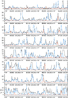 |
Fig. C.1 Same as Fig. 4 but for CH3NH2, υ = 0. |
| In the text | |
Current usage metrics show cumulative count of Article Views (full-text article views including HTML views, PDF and ePub downloads, according to the available data) and Abstracts Views on Vision4Press platform.
Data correspond to usage on the plateform after 2015. The current usage metrics is available 48-96 hours after online publication and is updated daily on week days.
Initial download of the metrics may take a while.