| Issue |
A&A
Volume 677, September 2023
|
|
|---|---|---|
| Article Number | A132 | |
| Number of page(s) | 10 | |
| Section | The Sun and the Heliosphere | |
| DOI | https://doi.org/10.1051/0004-6361/202244129 | |
| Published online | 18 September 2023 | |
The nature of the solar wind electron temperature and electron heat flux
II. Case of a spiral interplanetary magnetic field
1
Department of Chemistry, University of British Columbia, Vancouver V6T 1Z1, Canada
e-mail: This email address is being protected from spambots. You need JavaScript enabled to view it.
2
Space Sciences Laboratory, University of California, Berkeley, CA 94720, USA
e-mail: This email address is being protected from spambots. You need JavaScript enabled to view it.
Received:
27
May
2022
Accepted:
22
February
2023
Abstract
Aims. We aim to analyze the solutions of the solar wind electron energy equation in a spherical expansion with a spiral interplanetary magnetic field (IMF), a radial power law of the electron heat flux with a constant index α, and a constant or a smooth increase of the solar wind speed.
Methods. Generic analytical electron temperature profiles for constant co-latitude of the radial vector r and different power law indices of the electron heat flux are established. We concentrate on the solution of the energy equation for an expansion in the heliospheric equatorial plane. We define a critical electron heat flux that is a fraction of the electron thermal energy convected at the solar wind speed and plays a crucial role in the electron energy equation solution.
Results. When the electron heat flux density is equal to the critical heat flux, the electron temperature is driven by the dissipation of the electron heat flux and the effect of the IMF. This corresponds to a heat dissipation dominated (HDD) expansion of the electrons. When the electron heat flux is not equal to the critical electron heat flux, three effects drive the electron temperature evolution: an adiabatic cooling, the dissipation of the electron heat flux and the spiral IMF effect. These contributions are quantitatively evaluated along the radial expansion. For a same electron heat flux and solar wind velocity, we show an important effect, that the solar wind electron temperature with a spiral IMF is higher than with a radial IMF up to some large radial distances, and that this difference increases with an increasing power law index α up to −2. Based on the phenomenological energy equation, we show that the Spitzer and Härm law is approximately verified in a spiral IMF for moderate radial distances from the Sun lower than 2 AU, with an electron heat flux power law index a little lower than −2.40 and an electron temperature with a power law a little higher than −0.40. A complete study requires the solution of the electron fluid equation for different solar wind speed profiles. The study of data collected on the Ulysses mission, along a portion of a southward high-latitude orbit, needs a specific analysis because a large variation of the co-latitude is observed along that orbit leg. From this study, we conclude that the dissipation of the electron heat flux between 1.52 and 2.3 AU cannot sustain the measured total electron temperature in this distance range; we show that the core-strahl electron population has a temperature driven by the heat flux dissipation between 1.52 and 2.3 AU, and that this core-strahl temperature profile has the property of an HDD expansion.
Conclusions. The results, in Parts 1 and 2, suggest we should study the energetics of the solar wind core-strahl electron population as a whole and revisit the Spitzer and Härm law corresponding to this population while taking into account the spiral IMF.
Key words: Sun: heliosphere / solar wind / plasmas / conduction / magnetic fields / methods: analytical
© The Authors 2023
 Open Access article, published by EDP Sciences, under the terms of the Creative Commons Attribution License (https://creativecommons.org/licenses/by/4.0), which permits unrestricted use, distribution, and reproduction in any medium, provided the original work is properly cited.
This article is published in open access under the Subscribe to Open model. This email address is being protected from spambots. You need JavaScript enabled to view it. to support open access publication.
1. Introduction
In Paper I (Hubert et al. 2023), we set up a phenomenological model of the solar wind electron energy equation in spherical expansion, with the assumption of a radial interplanetary magnetic field (IMF) and an electron heat flux given by a radial power law with a constant index. The energy equation is solved explicitly in a range of radial distances where the solar wind V is a constant; we show that this solution can be extended directly to a range of radial distances with a smooth increase in solar wind speed such that r V−1 ∂V/∂r is equal to a positive constant, with r being the radial distance. We define a critical electron heat flux that plays a crucial role in the solution of the energy equation. If the electron heat flux is equal to the critical electron heat flux at some radial origin, the electron temperature evolution is controlled uniquely by the dissipation of the heat flux. This defines a heat dissipation dominated (HDD) expansion of the solar wind electrons. If the electron heat flux is not equal to the critical heat flux, both an adiabatic cooling and the dissipation of the electron heat flux govern the electron temperature evolution. We provide generic analytical electron temperature laws for different power law indices of the electron heat flux; from these generic analytical laws, the adiabatic cooling and the heat flux dissipation effects are quantitatively evaluated. Revisiting the solution of the electron energy equation with the Spitzer & Härm (1953, hereafter SH) conduction law as a closure of the equation, we establish that the electron temperature evolution is ∝r−0.4 in the range of radial distances where the solar wind speed is constant or smoothly increasing. A necessary condition for the SH law to be valid along large radial distance is that the power law index of the electron heat flux is equal to −2.4. An application of the generic electron temperature law to kinetic numerical simulations with a radial IMF describes the characteristics of the electron temperature and its evolution with precision (Landi et al. 2012). In these kinetic simulations the electron distribution functions display the typical core-strahl features observed in solar wind data (e.g. Feldman et al. 1975; Pilipp et al. 1987a,b; Maksimovic et al. 2005; Salem et al. 2023).
In Paper II, we extend the phenomenological model of the solar wind energy equation set up in Paper I to include a spiral IMF and a constant or a smooth increase solar wind speed. The IMF topology is defined by the spiral model developed by Parker (1958). A number of studies pointed out the effect of a spiral IMF on the solar wind temperature radial profile in one-fluid approach (Urch 1969; Gentry & Hundhausen 1969). In a two-fluid approach, Wolff et al. (1971) showed that the electron temperature decrease in the heliospheric equatorial plane is lower than in a similar model with a radial IMF. Figure 3.12 in Hundhausen (1972) compares the temperature profile of the one-fluid model in a radial IMF (Whang & Chang 1965) to the one-fluid model with a spiral IMF. A lower temperature decrease is obtained in a spiral IMF up to about 6 AU, and at further radial distances the opposite is obtained, that is a larger temperature decrease in a spiral IMF. In the exospheric approach, Pierrard et al. (2001) showed that the electron temperature in the heliospheric equatorial plane with a spiral IMF is higher at radial distance between 100 Rs and the limit of their calculations, 300 Rs, were Rs is the Sun radius, than in a radial IMF where the electron temperature is provided by Meyer-Vernet & Issautier (1998). Other solar wind models include a spiral IMF but do not comment on the consequences on the electron temperature or the heat flux characteristics such as the multi-moment model by Li (1999). In the study by Li (1999), the electron model includes a heat flux equation with a spiral IMF in the heliospheric equatorial plane. Their results for a fast solar wind show, for example in their model 3, that the electron heat flux is a radial power law with an index around −2.6, in the range of radial distances from 20 Rs to 300 Rs. The electron temperature decreases also as a radial power law, with an index around −0.4 in the same range of radial distances, which suggest an effect of the spiral IMF if we compare this decrease to the ones obtained in Paper I with a radial IMF. The electron temperature radial profiles being impacted by the spiral IMF, one needs to specifically address the validity of the SH law. The goal is to predict electron heat-flux power law models that verify the SH law along large radial distances from the Sun, as obtained in Paper I.
The assumption that the electron heat flux is a power law along large radial distances from the Sun is supported by electron measurements made in the solar wind by many spacecraft missions such as Helios or Ulysses. Data from the Helios 1 and 2 missions, collected in the ecliptic plane from 0.3 to 1 AU, display a wide range of power law indices of the electron heat flux, relevant to the slow and fast solar wind (Pilipp et al. 1990). Analyzing the energetics of solar wind electrons in Helios 1 and 2 data, Pilipp et al. (1990) concluded that for the relatively uniform high-speed solar wind, the total electron temperature cannot be explained only by the electron heat flux dissipation. They suggest that the electrons undergo external heating processes. Recently, Štverák et al. (2015), revisiting the Helios 1 and 2 data, concluded that the electrons do not need a significant heating mechanism to explain the observed total temperature gradient in the fast solar wind. We stress that these authors did not address the role of the heat flux dissipation with respect to the thermal evolution of the different populations of the solar wind electron distribution functions.
During a period of minimum solar activity, interesting plasma measurements have been obtained on the Ulysses mission from the south solar pole to the north solar pole. Indeed, Issautier et al. (1998) identified a period of stationary fast solar wind with a flow speed of around 750 km s−1 (McComas et al. 2000, 2003) and an electron core density decreasing as ∝r−2, while the core electron temperature, the total electron temperature (Le Chat et al. 2011), and the electron heat fluxes (Scime et al. 1999) follow radial power laws southward of 40° heliospheric latitudes at distances from 1.52 to 2.30 AU. Le Chat et al. (2011) analyzed the total electron temperature using Ulysses data, and their power law fit to the data yields uncertainties comparable to a fit using the exospheric model by Meyer-Vernet & Issautier (1998). This exospheric model contains an adiabatic contribution of the core component of the electron distribution function and an isothermal contribution with an equal weight at 1 AU. We note that the core electron temperature ∝r−0.64 (Issautier et al. 1998) is far from an adiabatic decrease and that the large variation from 40° to 80°S in the heliospheric latitude is not taken into account in the temperature analysis by Le Chat et al. (2011).
In Sect. 2, we study the solution of the electron energy equation with a spiral heliospheric IMF and a radial power law for the electron heat flux. We define the conditions to obtain an analytical solution of the phenomenological electron energy equation along heliospheric trajectories. We analyze, in detail, the case of a trajectory in the heliospheric equatorial plane, and we stress the differences of the solution properties with respect to the radial IMF case. In Sect. 3, we address the validity of the SH law with a spiral IMF in a range of large radial distance from the Sun. Section 4 is devoted to a specific analysis of the electron energy equation that applies to data collected at high heliospheric latitude on the Ulysses mission, along an orbit with a variable co-latitude. We look for some rationale between the electron heat flux dissipation and the balance of energy of the different populations composing the electron velocity distribution function, namely the total temperature of the three populations defined as a whole and the temperature of the core-strahl population. We discuss the results in Sect. 5, and Sect. 6 is devoted to a conclusion of this study.
2. Phenomenological electron energy equation model
We set up a solar wind model composed of electrons and protons with isotropic temperatures. Charge neutrality and zero electrical current conditions are assumed through the equality of the electron and proton densities, such that ne = np = n, and through the equality of the electron and proton bulk flow speeds, such that Ve = Vp = V. We consider a spherical expansion with a flow tube cross-section of S = r2, where r is the radial distance from the center of the Sun. The stationary radial equation describing the evolution of the electron temperature Te is
 (1)
(1)
In this equation, k is the Boltzmann constant, Tp is the proton temperature, me and mp are, respectively, the electron and the proton mass, qe is the electron heat flux intensity at the radial distance r, and νep is the electron-proton collision frequency. The electron heat flux vector is qe(r) = qe(r)b, where b is the local direction of the unit vector of the IMF in r. The angle between the radial vector r and the IMF direction in r is ϕ(r); in Eq. (1), the cosine of this angle appears because the electron heat flux contribution needs to be projected along the radial vector r.
The topology of the IMF is defined by Parker’s model (Parker 1958), which uses the following relations: tanϕ(r) = (ω r/V) sin θ for r > 10 Rs and tanϕ(r) = 0 for r ≤ 10 Rs, where r is the modulus of r, Rs is the solar radius, ω = 2.7 × 10⁻⁶ rad s−1 is the Sun’s rotation angular velocity, and θ is the heliocentric co-latitude of r. For a constant solar wind speed and a constant co-latitude different from 0 or 180°, the angle ϕ(r) increases for an increasing radial distance of r > 10 Rs; the larger the flow speed, the smaller the angle ϕ(r) for a given distance r. For a given solar wind speed and a given radial distance larger than 10 Rs, the angle ϕ(r) increases with a co-latitude increasing from 0 to 90° or a co-latitude decreasing from 180 to 90°. For a co-latitude θ equal to 0 or 180°, the angle ϕ(r) is equal to zero degrees, and then the IMF is radial. The function cos ϕ(r) in Eq. (1) can be complicated along an orbit with variation of the heliospheric co-latitude with the radial distance; an example is provided by Ulysses’ solar pole-to-pole journey in 1994–1995 (McComas et al. 2000).
We analyze the solution of the electron thermal energy governed by Eq. (1), where the electron heat flux intensity is qe(r) = q0 (r/r0)α with q0 = qe(r0) and where the power law index α is a constant. We want to compare the predictions derived from Eq. (1) to solar wind data that are currently available at large radial distances from the Sun. We consider the solution of Eq. (1) for radial distances r ≥ r0, where the flow speed V(r) = V(r0) = V0 is constant; the case of a smoothly increasing flow speed is commented on at the end of this section. The small electron-to-proton mass ratio and the low value of the electron-proton collisional frequency at radial distances larger than some 0.1 AU imply that the thermal energy exchange between these two populations is very small (Hartle & Sturrock 1968) and is ignored in Eq. (1), which we also did in Paper I. With the electron heat flux model above, the explicit expression of cos ϕ(r), (Parker 1958), and a spherical expansion with n V = n0 V0 (r/r0)−2 where n0 = n(r0), we can rewrite Eq. (1) as
![Mathematical equation: $$ \begin{aligned} \frac{\partial T_{\rm e}}{\partial r} + \frac{4\,T_{\rm e}}{3\,r}+ \frac{2\,q_0\,\,r_{0}^{-(\alpha +2)}}{3\,n_0\,k\,V_0}\,\frac{\partial }{\partial r}\left(\frac{r^{\alpha +2}}{\left[1+(\omega \,r\,\sin \theta /V_0)^2\right]^{1/2}}\right) = 0. \end{aligned} $$](/articles/aa/full_html/2023/09/aa44129-22/aa44129-22-eq2.gif) (2)
(2)
Equation (2) is a first-order, linear, non-homogeneous, differential equation, where the electron temperature evolution is coupled to the heat flux through the third term on the left. With Cs a constant of integration, the electron temperature is given by
![Mathematical equation: $$ \begin{aligned} T_{\rm e}(r) = r^{-4/3} \left[C_{\rm s} - \frac{2\,q_0 r_0^{-\alpha -2}}{3\,n_0\,k\,V_0}\,I_{\rm s}(\alpha ,\omega ,\theta ,V_0,r)\right], \end{aligned} $$](/articles/aa/full_html/2023/09/aa44129-22/aa44129-22-eq3.gif) (3)
(3)
where
![Mathematical equation: $$ \begin{aligned} I_{\rm s}(\alpha ,\omega ,\theta ,V_0,r) = \int \mathrm{d}r\;r^{-4/3}\;\frac{\partial }{\partial r}\left(\frac{r^{\alpha +2}}{[1+(\omega \,r\,\sin \theta /V_0)^2]^{1/2}}\right)\cdot \end{aligned} $$](/articles/aa/full_html/2023/09/aa44129-22/aa44129-22-eq4.gif) (4)
(4)
The constant of integration defined from initial conditions at a radial distance r0 is:
 (5)
(5)
The electron temperature in Eq. (3) exhibits two contributions, as long as Cs is not equal to zero. The first contribution is the adiabatic cooling, and the second contribution includes both the dissipation of the electron heat flux and the effect of the spiral IMF embedded in the solar wind flow. The integral in Eq. (4) depends on the electron heat flux power law index, the angular rotation velocity of the Sun, the solar wind speed, and any specific trajectory in the heliosphere. It is a complex function that does not reduce to a unique expression if the co-latitude depends on the radial distance. However, for a trajectory with a constant heliocentric co-latitude of θ0, we obtain generic expressions. With α ≠ −10/3, we obtain
![Mathematical equation: $$ \begin{aligned} I_{\rm s}(\alpha ,\omega ,\theta _0,V_0,r) =&3\;\frac{r^{\alpha +10/3}}{3\alpha +10}\left[(\alpha +1)F\left(\frac{1}{2},\alpha ,\omega ,\theta _0,V_0,r\right)\right.\nonumber \\&+ \left. F\left(\frac{3}{2},\alpha ,\omega ,\theta _0,V_0,r\right) \right], \end{aligned} $$](/articles/aa/full_html/2023/09/aa44129-22/aa44129-22-eq6.gif) (6)
(6)
in which F(1/2, α, ω, θ0, V0, r) and F(3/2, α, ω, θ0, V0, r) are defined from the generalized hypergeometric series (Abramowitz & Stegun 1965) as
 (7)
(7)
and
 (8)
(8)
For α = −10/3 with a constant co-latitude, the integral in Eq. (4) is
![Mathematical equation: $$ \begin{aligned} I_{\rm s}\left(\frac{-10}{3},\omega ,\theta _0, V_0, r\right) =&-\frac{4}{3}\log r + \frac{V_0}{\sqrt{V_0^2 + \omega ^2\,r^2\,\sin ^2\theta _0}}\nonumber \\&+ \frac{4}{3}\log \left[V_0\left(V_0 + \sqrt{V_0^2 + \omega ^2\,r^2\,\sin ^2\theta _0}\right)\right]. \end{aligned} $$](/articles/aa/full_html/2023/09/aa44129-22/aa44129-22-eq9.gif) (9)
(9)
With a defined co-latitude of θ0, the electron temperature in Eq. (3) is therefore analytical. By setting the co-latitude as equal to 0° or 180°, that is, sin θ0 = 0 in Eqs. (6) and (9), we obtain the corresponding quantities derived in Paper I that are devoted to the radial IMF topology. In Paper II, we consider a trajectory in the heliospheric equatorial plane with the co-latitude equal to 90°, that is with sin θ0 = 1. The expression in Eq. (4), where we omit θ0 (θ0 = 90°), is then
 (10)
(10)
As noted above, we distinguished two cases with respect to the power law index: α ≠ −10/3 and α = −10/3.
2.1. Case with α ≠ −10/3
From Eqs. (6) and (10), we obtain
![Mathematical equation: $$ \begin{aligned} I_{\rm s}(\alpha ,\omega ,V_0,r) =&3\,\frac{r^{\alpha +10/3}}{3\alpha +10} \,\left[(\alpha +1)\,F\left(\frac{1}{2},\alpha ,\omega ,V_0,r\right)\right. \nonumber \\&+ \left.F\left(\frac{3}{2},\alpha ,\omega ,V_0,r\right)\right], \end{aligned} $$](/articles/aa/full_html/2023/09/aa44129-22/aa44129-22-eq11.gif) (11)
(11)
with F(1/2, α, ω, V0, r) and F(3/2, α, ω, V0, r), respectively, defined in Eqs. (7) and (8), with sin θ0 = 1. For α > −2, the function Is(α, ω, V0, r) in Eq. (11) has positive values for radial distances lower than about 2 AU and becomes abruptly negative at larger radial distances. Then, the electron temperature evolution also shows an abrupt increase without a clear physical meaning; therefore, in the remainder of this section we consider α ≤ −2. As long as −10/3 < α ≤ −2, the properties of the generalized hypergeometric series, F(1/2, α, ω, V0, r) and F(3/2, α, ω, V0, r), are similar with respect to the radial distance, with F(1/2, α, ω, V0, r)≥F(3/2, α, ω, V0, r). They decrease from around 1.0 at radial distances r < 0.2 AU to 0.0 at very large radial distances. They both converge to 1.0 whatever the radial distance, when the power law index α converges to −10/3. From the relative values of F(1/2, α, ω, V0, r) and of F(3/2, α, ω, V0, r), we show that Is(α, ω, V0, r) in Eq. (11) is negative. For α < −10/3, we have F(1/2, α, ω, V0, r)≤F(3/2, α, ω, V0, r) and these two functions increase from 1.0 at r < 0.2 AU to values larger than 1.0 with an increasing radial distance; we show that the quantity Is(α, ω, V0, r) in Eq. (11) is then positive. The constant of integration in Eq. (5) with sin θ0 = 1 is
 (12)
(12)
2.2. Constant Cs = 0
A necessary condition for the constant Cs to be equal to zero is that the power law index α lies in the range of −10/3 < α ≤ −2. With Cs equal to zero, the adiabatic contribution to the electron temperature in Eq. (3) disappears, and the electron temperature is driven entirely by the dissipation of the electron heat flux and the effect of the spiral IMF. This defines a heat dissipation dominated (HDD) expansion of the electrons in the equatorial heliospheric plan with a spiral IMF with a temperature of
 (13)
(13)
where the function J(α, ω, V0, r) is defined as follows:
 (14)
(14)
With Cs = 0, the electron heat flux intensity at r0 takes a specific expression in terms of the electron thermal energy at r0 convected at the solar wind speed; indeed, from Eq. (12), we have
 (15)
(15)
It is straightforward to show that as Eq. (15) is verified at r0, its generalization to any radial distance r is also verified.
The analysis of the function J(α, ω, V0, r) in Eq. (14), from the properties of its constitutive functions, shows that it converges to zero as the power law index α converges to −2. Therefore, the electron heat flux in Eq. (15) increases to infinity as α converges to −2; it is equal to the free streaming heat flux for a certain power law index of α1 < −2. As the free streaming heat flux is the maximum possible heat flux, this implies a second constraint on the electron heat flux power law indices α ≤ α1, in order to define a HDD expansion. Then, the range of power law indices for an HDD expansion is limited to −10/3 < α ≤ α1.
The electron temperature in Eq. (13), in an HDD expansion of the electrons with a spiral IMF, is not equal to the electron temperature in a radial IMF. J−1(α, ω, V0, r0)⋅J(α, ω, V0, r) is the ratio of Te in a spiral IMF in the heliospheric equatorial plane over Te in a radial IMF. This ratio is a function of the radial distances, r0 and r, of the solar wind speed and of the power law index α. Figure 1 shows this ratio for a solar wind flow speed of 550 km s−1 and different indices α in the range of radial distances from 0.1 to 50 AU. For α = −3.3, J−1(α, ω, V0, r0)⋅J(α, ω, V0, r) is nearly equal to 1.0 whatever the radial distance because the constitutive functions of J(α, ω, V0, r) converge toward 1.0 whatever the distance when α converges to −10/3; then, the electron temperature profiles in a radial, and in a spiral IMF are the same and vary as ∝r−1.3.
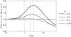 |
Fig. 1. Ratio J−1(α, ω, V0, r0)⋅J(α, ω, V0, r) as a function of radial distance from r0 = 0.1 AU up to 50 AU, for a solar wind speed of 550 km s−1 and for different values of the electron heat flux power law index α. |
For α = −2.9, the ratio J−1(α, ω, V0, r0)⋅J(α, ω, V0, r) in Fig. 1 is a little higher than 1.0 up to 4 AU and decreases to values lower than 1.0 at larger radial distances; therefore, at distances larger than 4 AU the electron temperature in a spiral IMF is lower than in a radial IMF. The ratio J−1(α, ω, V0, r0)⋅J(α, ω, V0, r) increases up to around 3 AU and then decreases to values lower than 1.0 at some larger radial distances for α = −2.4 and α = −2.2. For α = −2.4, the maximum is 1.4 around 3 AU, and the ratio decreases to values lower than 1.0 further than 8 AU; for α = −2.2, the maximum is around 2.1 at 3 AU, and the ratio decreases to values lower than 1.0 further than 20 AU. These ratios that are higher than 1.0 and later lower than 1.0 indicate that with the same electron heat flux, the electron temperature in a spiral IMF is higher than the electron temperature in a radial IMF, up to distances r1 depending on the power law index α; at larger distances, the opposite trend is obtained, that is the electron temperature in a spiral IMF is lower than in a radial IMF. The distance r1 increases with an increasing power law index α. For a slow solar wind speed of 350 km s−1 and a fast solar wind speed of 750 km s−1, the ratios J−1(α, ω, V0, r0)⋅J(α, ω, V0, r) have the same general properties as functions of the power law index α and the radial distance. Indeed, the respective maximum of J−1(α, ω, V0, r0)⋅J(α, ω, V0, r) for α = −2.4 and α = −2.2 is the same for a slow solar wind and a fast solar wind. However, for a slow (fast) solar wind the maximum is located at smaller (larger) radial distances, and the ratios decrease to lower values than 1.0 at smaller (larger) radial distances than for a solar wind velocity of 550 km s−1.
Figure 2 shows electron temperature profiles for a solar wind speed of 550 km s−1 from 0.1 to 50 AU in HDD expansion, in a radial IMF (see Paper I, Eq. (6)), and in a spiral IMF. The chosen electron temperature of 5 × 10⁵ K at r0 = 0.1 AU is realistic with respect to early measurements on the Parker Solar Probe (Halekas et al. 2020; Moncuquet et al. 2020). Then, we calculate that an HDD expansion is defined in the range of α with −10/3 < α ≤ −2.16, and we consider three electron heat flux power law indices in this range, α = −2.9, α = −2.4, and α = −2.2. The profiles in a radial IMF show a decrease of ∝rα + 2, but in a spiral IMF they are more complex, except for α = −2.9, where the two profiles cannot be distinguished. The electron temperature in a spiral IMF is, respectively, higher than in a radial IMF up to a distance of r1 ≃ 9 AU for α = −2.4 and r1 ≃ 20 AU for α = −2.2; at larger distances, the opposite is noted. For α = −2.2 in a spiral IMF, the electron temperature displays a significant peak around 2 AU, with the temperature higher than at the origin at 0.1 AU. It is the result of the important spiral IMF effect as seen for α = −2.2 in Fig. 1 and the dissipation effect of the electron heat flux, which decreases slowly as ∝r−2.2.
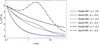 |
Fig. 2. Electron temperature profiles in HDD expansion, for a radial IMF, and for a spiral IMF for a solar wind speed of 550 km s−1 from 0.1 to 50 AU. Three electron heat flux power law indices are considered: α = −2.9, −2.4, and −2.2. |
2.3. Constant Cs ≠ 0
As Cs ≠ 0, Eq. (15) is not verified, we define a critical electron heat flux in a spiral IMF as
 (16)
(16)
Let us first consider the case Cs < 0. The constant of integration Cs, defined in Eq. (12), is negative if two simultaneous conditions are met: first the quantity Is(α, ω, V0, r0) must be negative, which requires the power law index to satisfy −10/3 < α ≤ −2, and the second condition, obtained by introducing the critical heat flux into the constant Cs as  , is qe(r0) > qcs(r0). This inequality is valid whatever the radial distance, r; as long as it is verified at r0, it also induces a limitation on the range of acceptable power law indices −10/3 < α ≤ α1, because for α > α1, the critical heat flux in Eq. (16) is important and it is larger than the free streaming heat flux. The electron temperature is then
![Mathematical equation: $$ \begin{aligned} T_{\rm e}(r) =&\left[1-\frac{q_{\rm e}(r_0)}{q_{\rm cs}(r_0)}\right]T_{\rm e}(r_0)\left(\frac{r}{r_0}\right)^{-4/3}\nonumber \\&+\frac{q_{\rm e}(r_0)}{q_{\rm cs}(r_0)}\,T_{\rm e}(r_0)\,J^{-1}(\alpha ,\omega ,V_0,r_0)\cdot J(\alpha ,\omega ,V_0,r)\,\left(\frac{r}{r_0}\right)^{\alpha +2}. \end{aligned} $$](/articles/aa/full_html/2023/09/aa44129-22/aa44129-22-eq18.gif) (17)
(17)
The electron temperature has a negative adiabatic contribution and a positive contribution due to the dissipation of the electron heat flux. At large radial distances, the main contribution is the dissipation of the electron heat flux in the second term of Eq. (17), because α + 2 > −4/3. We do not show figures for this situation, which is not realistic because it implies a large electron heat flux higher than the critical electron heat flux.
Now we consider the case with Cs > 0. There are two possibilities for the constant Cs to be positive. First, for −10/3 < α ≤ −2 with the condition qe(r0) < qcs(r0), which is shown to be valid at any radial distance r as long as it is valid at r0, and, second, for α < −10/3, because for such a value the quantity Is defined in Eq. (11) is positive. In these two scenarios the electron temperature in Eq. (17) has a positive contribution from the adiabatic term. In the first situation with −10/3 < α ≤ −2 and qe(r0) < qcs(r0), the second contribution in Eq. (17) is positive and is dominant at large radial distances as a result of the dissipation of the electron heat flux. For α < −10/3, the second contribution to the electron temperature is negative, because the critical electron heat flux is negative; at large radial distances, the adiabatic contribution is dominant.
In Fig. 3, the electron temperature profiles are shown in a radial and in a spiral IMF with a realistic electron heat flux intensity equal to 1/3 of the electron free streaming heat flux at 0.1 AU (Salem et al. 2003; Halekas et al. 2021). The critical heat flux is calculated from Eq. (16) for α = −2.9 and α = −2.2 with a solar wind speed of 550 km s−1 and an electron temperature of 5 × 10⁵ K at 0.1 AU. For α = −2.9, the critical heat flux is much lower than the free streaming heat flux; therefore, the contribution of the adiabatic cooling is important and negative. For α = −2.2, the contribution of the adiabatic cooling is positive. The electron temperature in a radial IMF is defined in Paper I in Eq. (9) and in a spiral IMF in Eq. (17). For α = −2.9, the two temperatures cannot be distinguished and decrease smoothly. For α = −2.2, while the electron temperature decreases monotonically in a radial IMF, in a spiral IMF the temperature shows a local peak around 2 AU and then decreases to values smaller than the radial temperatures at distances larger than 20 AU. For α = −2.4, the critical heat flux is slightly smaller than the considered heat flux at 0.1 AU, which is 1/3 of the free-streaming heat flux. Therefore, the adiabatic cooling is significantly small and the relevant temperatures for α = −2.4 are the same as the ones given in Fig. 2.
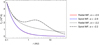 |
Fig. 3. Electron temperature evolution in a radial and spiral IMF with the power law indices α = −2.9, α = −2.2, and an electron heat flux intensity equal to 1/3 of the free streaming electron heat flux at 0.1 AU. |
2.4. Case with α = −10/3
In the heliospheric equatorial plane, Eq. (9) takes the following form:
![Mathematical equation: $$ \begin{aligned} I_{\rm s}(-10/3,\omega ,V_0,r) =&-\frac{4}{3}\,\log (r) + \frac{V_0}{\sqrt{V_0^2+\omega ^2\,r^2}}\nonumber \\&+ \frac{4}{3}\,\log \left[V_0\,\left(V_0+\sqrt{V_0^2+\omega ^2\,r^2}\right)\right]\cdot \end{aligned} $$](/articles/aa/full_html/2023/09/aa44129-22/aa44129-22-eq19.gif) (18)
(18)
The sign of the expression in Eq. (18) depends on the solar wind speed and on the radial distance. It is positive for a slow solar wind speed and a radial distance lower than 15 Rs and then it becomes negative for larger radial distance; for the fast solar wind, it is positive whatever the radial distance. With the definition of the critical electron heat flux for α = −10/3, which we distinguish from the case with α ≠ −10/3 in Eq. (16), we have
 (19)
(19)
The expression of the electron temperature is obtained from the initial conditions at r0 as
![Mathematical equation: $$ \begin{aligned} T_{\rm e}(r) =&\left[1-\frac{q_{\rm e}(r_0)}{q^{\prime }_{\rm cs}(r_0)}\right]\, T_{\rm e}(r_0)\left(\frac{r}{r_0}\right)^{-4/3}\nonumber \\&+ \frac{q_{\rm e}(r_0)}{q^{\prime }_{\rm cs}(r_0)}\,T_{\rm e}(r_0)\;\frac{I_{\rm s}(-10/3,\omega ,V_0,r)}{I_{\rm s}(-10/3,\omega ,V_0,r_0)}\,\left(\frac{r}{r_0}\right)^{-4/3}. \end{aligned} $$](/articles/aa/full_html/2023/09/aa44129-22/aa44129-22-eq21.gif) (20)
(20)
The electron temperature has two contributions: The first is adiabatic, while the second is non-adiabatic, because the function Is(−10/3, ω, V0, r) is a function of the radial distance.
2.5. Case of a non constant solar wind speed
The solutions of the empirical electron energy equation, with the assumption of a constant solar wind speed, can be extended to the range of radial distances and speed, such that r V−1∂V/∂r = δ, where “δ” is a small and positive constant to fit the solar wind speed profile. For instance, δ = 0.14 in the very slow solar wind between 0.3 and 1.0 AU (Maksimovic et al. 2020). In the high-latitude fast solar wind, the flow speed is more or less constant at around 750 km s−1 (see Sect. 4) and this yields δ ∼ 0.
Yeh (1971) noted that the energy equation structure is qualitatively the same, whether it uses a solar wind speed of the form V(r) = V(r0) (r/r0)δ or a constant solar wind speed V. Then the coefficient 4/3 in the second term of Eq. (2) is replaced by (4 + 2δ)/3, and the solution of the new energy equation is qualitatively the same as the solution in Sects. 2.2 and 2.3. Calculations show that the quantities in Fig. 1 calculated with different flow speeds for a given electron heat flux power law index have a very close maximum located at nearly the same radial distance. Similarly, the critical electron heat flux in Eq. (16) is not much impacted either. These two quantities being constitutive of the electron temperature in Eq. (17), we find that for a given power law index of the electron heat flux the electron temperature profile is not significantly modified for a smoothly increasing flow speed.
3. The SH thermal conduction law in a spiral IMF
We want to know the conditions required for the SH law to be verified in the solar wind within a spiral IMF along large radial distances from the Sun. Moreover, with the assumption that the electron heat flux is a radial power law, we want to find out whether the requirement
 (21)
(21)
is verified (Hundhausen 1972) for a given index α, with κ constant and Te the electron temperature established in Sect. 2. With the electron temperature in an HDD expansion in Eq. (13), which is not a radial power law with a constant index, we find that no electron heat flux as a power law meets the above requirement whatever the radial distance is. For a radial IMF, we find that with α = −2.4 the above requirement is verified (see Sect. 3 in Paper I). Considering Fig. 2 and the temperature profiles in a radial and in a spiral IMF for α = −2.4, one notes that for radial distances between 1 and 3 AU, for example, the right hand side in Eq. (21) is much higher than the left hand side in the spiral IMF case, and it is the opposite at distances larger than 10 AU.
In a spiral IMF, the electron temperature profile obtained with α = −2.4 in Fig. 2 is very similar to the temperature profile obtained in the fluid equation by Gentry & Hundhausen (1969; see Fig. 3.12 in Hundhausen 1972), while the solar wind speed is different in these two studies. Therefore, the SH law in Eq. (21), within the temperature profile obtained by Gentry & Hundhausen (1969), is not a radial power law either. Nevertheless, we find that the SH law is nearly verified in a spiral IMF for an electron heat flux with a power law index α a little lower than −2.4 and an electron temperature power law index β a little higher than −0.40 for a radial distance lower than 2 AU, as long as it is verified in a given distance within 2 AU.
4. Analysis of high-latitude solar wind observations
We analyze observations made on Ulysses in the fast solar wind at trajectory southward of heliospheric latitudes of 40° to 80°, from 1.52 to 2.30 AU. We select these observations as they display, for a rather long distance, a complete set of plasma parameters in a steady, fast, solar wind speed of 750 km s−1 (McComas et al. 2003). The core electron density follows the radial law ∝r−2. The core electron temperature and the total electron temperature radial evolutions are, respectively, ∝r−0.64 (Issautier et al. 1998) and ∝r−0.53 (Le Chat et al. 2011). The electron heat flux follows a radial power law of ∝r−2.9 (Scime et al. 1999) in the same range of latitude and radial distance as the electron temperatures measured on Ulysses. The cosine of the angle ϕ(r) between the radial direction r and the IMF Parker model, along the Ulysses southward orbit can be modeled as a second-order polynomial or as a radial power law. They both provide the same electron temperature at 2.3 AU from the given temperature at 1.52 AU. We select the power law model as it is more straightforward, and we obtain cos ϕ(r) = cos ϕ0 ⋅ (r/1.52)γ with cos ϕ0 = cos ϕ(r0 = 1.52) and γ = 0.35. Introducing the expression of cos ϕ(r) in Eq. (1), with the assumption that the electron-proton collision frequency is equal to zero, we follow the developments in Paper I directly, from Eqs. (2) to (9). The critical electron heat flux at r0 = 1.52 AU is thus
 (22)
(22)
The specific electron temperature law along this Ulysses orbit leg is
![Mathematical equation: $$ \begin{aligned} T_{\rm e}(r) =&\left[1-\frac{q_{\rm e}(1.52)}{q_{\rm c}(1.52)}\right] \,T_{\rm e}(r_0)\,\left(\frac{r}{r_0}\right)^{-4/3}\nonumber \\&+ \frac{q_{\rm e}(1.52)}{q_{\rm c}(1.52)}\,T_{\rm e}(r_0)\,\left(\frac{r}{r_0}\right)^{\alpha +\gamma +2}. \end{aligned} $$](/articles/aa/full_html/2023/09/aa44129-22/aa44129-22-eq24.gif) (23)
(23)
Let us now apply this temperature law (Eq. (23)) to the total electron temperature measurements by Le Chat et al. (2011). The electron heat flux qe(1.52)≃2.0 μW m−2 measured at r0 = 1.52 AU (Scime et al. 1999) is much smaller than the critical electron heat flux for the total electron temperature obtained from Eq. (22), with the thermal energy measured at 1.52 AU and the solar wind speed of 750 km s−1; indeed, we obtain qc(1.52) = 5.7 μW m−2. The total electron temperature obtained from Eq. (23), with the required parameters defined at 1.52 AU and Tem(1.52) being the total electron temperature measured at 1.52 AU, is
 (24)
(24)
At the radial distance r = 2.30 AU, we obtain Te(2.30) = 0.64 Tem(1.52), while the measured total electron temperature is 25% higher, with Tem(2.30) = 0.80 Tem(1.52), (Le Chat et al. 2011).
The core-strahl electron temperature has not been measured on Ulysses, but the core temperature has (Issautier et al. 1998). Therefore, we assumed that the core-strahl temperature along this Ulysses leg is around 15% higher than the measured core electron temperature Tc(r), as observed in data from the Wind spacecraft at 1 AU in a fast solar wind of 700 km s−1 (Salem et al. 2023). Then, from this assumption of the core-strahl electron temperature that we note,  , we define a new critical electron heat flux at r0 = 1.52 AU; it is 2.04 μW m−2, a value a little higher than the electron heat flux observed at 1.52 AU. The core-strahl electron temperature is then predicted by the following law with a small adiabatic contribution:
 (25)
(25)
Figure 4 shows the core-strahl electron temperature from 1.52 AU to 2.3 AU obtained from Eq. (25) in solid line, with  K; with a dashed line, we plot the extrapolated core-strahl temperature assuming
  K. The solid curve in Fig. 4 is very close to the dashed curve, indicating that the predicted temperature law in Eq. (25) matches the Ulysses core-strahl electron temperature well. Indeed, at r = 2.30 AU we obtain
  , while the assumption of the core-strahl electron temperature provides
  using the expression of Tc(2.3) = 0.77 Tc(1.52), (see Issautier et al. 1998). With these two temperatures, Tc − s(2.30) and
  , being very close together, the prediction from Eq. (25) is accurate.
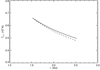 |
Fig. 4. Core-strahl electron temperature evolution from 1.52 to 2.3 AU obtained from Eq. (25) shown by the solid line and the extrapolated core-strahl temperature from the Ulysses core temperature shown by the dashed line. In 1.52 AU, the electron temperature is |

5. Discussion
The solution of the phenomenological electron solar wind energy equation in a spherical expansion, with a spiral IMF and a slowly increasing solar wind speed, is discussed with respect to the modulus and power law index of an electron heat flux model. We discuss the similarities and differences of the solutions in a spiral IMF and in a radial IMF. An application of the phenomenological model to the analysis of Ulysses data, obtained at high heliospheric latitude, enables us to discuss the role of the electron heat flux dissipation in shaping the electron distribution function.
As the stationary electron energy equation is analyzed at radial distances, where the solar wind speed is constant or smoothly increasing, the thermal energy exchange between electrons and protons or other heavy minor ions is ignored. We obtain a generic solution of the energy equation along trajectories as long as their co-latitude is constant. The solution of the phenomenological solar wind model, with a spiral IMF, is qualitatively the same as with a radial IMF. The main difference is a larger electron temperature with a spiral IMF than with a radial IMF up to a finite radial distance. This effect, maximum in the heliospheric equatorial plane, decreases with the co-latitude decreasing from 90° to 0° or increasing to 180°.
An important result is the definition of a critical electron heat flux in Eq. (16), qcs(r) = a(r) n(r) k V0 Te(r), in terms of a fraction of a(r) of the electron thermal energy convected at the solar wind speed, which sets up the electron temperature expression. Indeed, comparing the actual electron heat flux to the critical electron heat flux, at a given origin distance, r0, we quantitatively evaluate the adiabatic contribution and the electron heat flux dissipation contribution to the radial electron temperature evolution. If the actual electron heat flux is equal to the critical electron heat flux at r0, the electron temperature is completely controlled by the electron heat flux dissipation. We define this situation as an HDD expansion of the electrons. There are conditions in the range of power law indices α that allow an HDD expansion. A first condition, derived from the constant of integration equal to zero in the electron temperature solution, requires −10/3 < α ≤ −2; a second condition defines a power law index α1 through the equality of the critical heat flux to the free streaming heat flux. Then, the range of an electron heat flux power law index for an HDD expansion is −10/3 < α ≤ α1. With a spiral IMF, the fraction a(r) in Eq. (16), is a function of the power law index, α, of the flow speed and of the radial distance.
In an HDD expansion with a spiral IMF, the electron temperature profile with −10/3 < α < −2.7 is nearly the same as with a radial IMF (see Fig. 2 for α = −2.9). This result is important for an analysis of data collected in the ecliptic plane, as that, for example, by Scime et al. (1994), where the electron heat flux is a power law with α = −3.0. For a given α, with −2.7 ≤ α ≤ α1 and the same conditions at the origin, the electron temperature in an HDD model with a spiral IMF is higher than with a radial IMF up to a specific distance r1; beyond that distance, we note the opposite trend (see, in Fig. 2, the relevant curves for α = −2.4 and α = −2.2). These higher temperature values increase with α up to α1. The specific distance r1, from a few AU to tens of AU, is dependent on the power law index α and on the solar wind speed. Electron temperature profiles, very similar to those shown in Fig. 2 for α = −2.4, are presented in Fig. 3.12 (Hundhausen 1972), which shows solar wind temperature profiles obtained in one-fluid models. In these two figures, the temperatures in the radial IMF case decrease as ∝r−0.4. These temperature laws correspond to the solution of the one-fluid model by Whang & Chang (1965) and to our solution of the electron energy equation within the SH law as a closure (see Sect. 3 in Paper I). The profile of the one fluid temperature with a spiral IMF with respect to the radial IMF case was analyzed by Gentry & Hundhausen (1969) as an “inhibition conduction” with a spiral IMF, because these authors focused on the adiabatic temperature law at large distances. We stress that the increase of the electron temperature in a spiral IMF, with respect to the case of a radial IMF with the same power law for the electron heat flux, is an important characteristic not mentioned by Hundhausen (1972). The origin of this property lays in the third term of the energy Eq. (2), which quantifies the contribution of the electron heat flux dissipation. It is larger with a spiral IMF than with a radial IMF up to the distance r2 < r1. The distance r2 has the same properties with respect to the power law index α and the solar wind speed as the distance r1; it is about 0.5 r1, for example, for α = −2.4, and with a solar wind speed of 550 km s−1 one obtains r2 ≃ 4.2 AU while r1 ≃ 9 AU. At distances larger than r1 the temperature profile relevant to the spiral IMF decreases as ∝r−4/3 in Fig. 3.12 of Hundhausen (1972), while it decreases at a similar rate, ∝r−1.4, in Fig. 2. We note that the curves corresponding to α = −2.2 in Fig. 2 represent the electron temperature obtained with an unrealistic electron heat flux in the solar wind, a heat flux that is a little higher than the freely streaming heat flux at the origin.
The electron heat flux can be lower than the critical electron heat flux, at an original radial distance, r0, for −10/3 < α ≤ −2. Then, the electron temperature evolution is the result of an adiabatic contribution and of the electron heat flux dissipation, as seen in Eq. (17). The contribution of the electron heat flux dissipation is the same as in the HDD expansion, multiplied by the ratio of the actual electron heat flux to the critical electron heat flux at the radial distance r0. At large radial distances, the electron temperature is dominated by the dissipation of the electron heat flux. Examples of an electron heat flux lower than the critical electron heat flux are shown in Fig. 3, with a realistic electron heat flux equal to 1/3 of the freely streaming heat flux at the origin (Salem et al. 2003; Bale et al. 2013). For the case with α = −2.2, we note a local peak of the electron temperature with the spiral IMF case; this local peak is smaller than the unrealistic one in Fig. 2 obtained in an HDD model for α = −2.2. Our study shows that we can directly address the effect of the adiabatic cooling in solar wind data by comparing the measured electron heat flux to the critical heat flux at some original distance r0. If the measured electron heat flux is not equal to the critical electron heat flux, there is an adiabatic cooling: its weight is directly evaluated as 1 − qe(r0)/qcs(r0), and so is the weight of the electron heat flux dissipation contribution to the electron temperature evolution as qe(r0)/qcs(r0). We stress that up to now the adiabatic cooling contribution to the solar wind electron temperature has not been observed.
The electron heat flux can be larger than the critical heat flux, with −10/3 < α ≤ α1 or with α ≤ −10/3. In the first case, the adiabatic contribution to the electron temperature is negative; then, at a large radial distance, the electron temperature is dominated by the dissipation of the electron heat flux. In the second case, with α ≤ −10/3, the critical electron heat flux is negative, and the electron heat flux is obviously larger than this pseudo-critical heat flux. Then, the adiabatic contribution to the electron temperature is positive, while the contribution of the dissipation of the electron heat flux is negative. The electron temperature is dominated at large radial distance by the adiabatic contribution.
The solution of the empirical equation does not change significantly when extended to a smoothly increasing solar wind speed, as r V−1 ∂V/∂r = δ, where “δ” is a positive constant with δ ≪ 1. Therefore, data collected from the solar wind intense acceleration region, such as those collected by the Parker Solar Probe (Fox et al. 2016), can be analyzed with respect to the results obtained in the present work.
For a trajectory with a variable heliospheric co-latitude, the effect of the spiral IMF on the electron energy equation solution depends on the specific variation of the angle between the radial direction and the direction of the local IMF along the trajectory. Section 4 is devoted to this case, discussing the data collected by Ulysses at high southward heliospheric co-latitudes between 1.52 and 2.3 AU. To model the magnetic field along the Ulysses trajectory, we choose the Parker spiral model that Forsyth et al. (2002) showed to agree in a first-order to the observed IMF. Applying the specific electron temperature law in Eq. (23) to the total electron temperature from the original measurement at 1.52 AU, we predict, in Eq. (24), a temperature underestimated by 25% with respect to the observations at 2.30 AU. The total electron temperature predicted in Eq. (24) displays significant adiabatic cooling. We know that the evolution of the core temperature is not adiabatic (Issautier et al. 1998). Since the halo and strahl electrons are suprathermal populations, it is hard to decipher how the total electron temperature could include a robust adiabatic contribution (see Eq. (24)). This shows that the total electron temperature is more likely driven by competing processes including the dissipation of the electron heat flux and the formation of the halo electron population via wave-particle interactions (Pilipp et al. 1987a; Vocks et al. 2005; Salem et al. 2007; Verscharen et al. 2019). In the paradigm of the exospheric approach, the halo electron population is not predicted. Indeed, this theory predicts a truncated electron distribution far from the exobase. For the same data as those analyzed in Sect. 3, Le Chat et al. (2011) interpreted the total electron temperature in terms of the exospheric law derived by Meyer-Vernet & Issautier (1998). They concluded that the exospheric law is not more robust than the power law derived through a fitting process. We stress that the exospheric law contains two ingredients, an adiabatic contribution and an isothermal contribution, neither of which has ever been identified in the core-strahl-halo components of the electron distribution. In particular, the temperature of the Maxwellian core distribution decreasing as ∝r−0.64 is far from an adiabatic cooling (Issautier et al. 1998).
The core-strahl electron temperature in Ulysses data not being available, contrary to the core electron temperature, we made an assumption as of what the core-strahl electron temperature could be. This assumption is based on the core temperature and the core-strahl temperature measured on the Wind spacecraft in the fast solar wind (Salem et al. 2023). It is important to emphasize here that the electron core temperature evaluated at 1 AU from the Ulysses data, obtained from 1.52 AU up to 2.3 AU, is very close to the average core temperature measured by Wind in the fast solar wind at 1 AU (see Salem et al. 2023). So, this provides a reliable assumption for deducing the core-strahl electron temperature from 1.52 AU up to 2.3 AU. We find that the predicted core-strahl electron temperature at 2.3 AU from the assumed temperature at 1.52 AU, is very close to the assumed core-strahl electron temperature in 2.3 AU. We are left with the following picture. The core-strahl electron population does experience a very small adiabatic cooling, as seen in Eq. (25); it is part of an HDD expansion process whose temperature is almost solely controlled by the dissipation of the electron heat flux. The core-strahl electron temperature in Eq. (25) decreases with a power law index equal to −0.55, so it decreases more slowly than the measured core electron temperature with its power law index of −0.64 (Issautier et al. 1998). We suggest the core-strahl electron population should be considered as a whole in the evolution of the solar wind expansion, in the sense that their energetics cannot be tackled as separate components. If we had ignored the IMF spiral topology along this high co-latitude trajectory, assuming a radial IMF, the predicted core-strahl electron temperature at 2.30 AU would be badly estimated, as it would be nearly equal to the core-strahl electron temperature at r0 = 1.52 AU. The near equality of the electron temperature profiles, with a radial or a spiral IMF in the heliospheric equatorial plane, for an electron heat flux with a power law index of −10/3 < α < −2.7, does not apply for this high co-latitude trajectory, because the effective power law index of the electron heat flux in Eq. (22), −2.90 + γ = −2.55, is out of the range, −10/3 < α < −2.7.
Our core-strahl electron temperature prediction for these Ulysses data is only qualitative in nature. Indeed, we assumed that the core-strahl temperature is 15% higher than the core Ulysses electron temperature, which is based on the Wind data at 1 AU. The Ulysses measurements of the core temperature (Issautier et al. 1998) and the total temperature (Le Chat et al. 2011) are based on the analysis of the quasi-thermal noise (QTN) around the electron plasma frequency, via a QTN spectroscopy technique (Meyer-Vernet et al. 2017). While the core temperature determined by Issautier et al. (1998) is good, the determination of the total temperature by Le Chat et al. (2011) is overestimated. Therefore, the assumed core-strahl temperature between 1.52 and 2.3 AU, deduced from the core temperature, is a reasonably good approximation. Further studies need to consider the detailed contributions of the core-strahl population and the halo population to the electron heat flux and address the question of the control of the temperature evolution of the core-strahl population through the energy equation. What remains to be defined is whether the halo population plays a role in this process, while this population is collisionless, and if the halo contribution to the electron heat flux is as small in the fast solar wind as in the Wind data at 1 AU (Salem et al. 2023).
The validity of the SH law in the solar wind is based on the comparison of the observed electron heat flux to the predicted heat flux from the SH law, within the observed electron temperature along large radial distances (Scime et al. 1994). From our phenomenological energy equation in a spiral IMF, within a radial power law of the electron heat flux, we find that the heat flux predicted by the SH law with the calculated electron temperature is not a radial power law. We would obtain the same conclusion considering the temperature profile obtained in the electron fluid model (see Fig. 3.21 in Hundhausen 1972). So, with a spiral IMF, we are left with the question of whether there is an electron heat flux as a radial power law ∝rα providing, from the energy equation, the same electron temperature profile as the one predicted by the energy equation within the SH law as a closure. In Paper I, with a radial IMF, we find such an electron heat flux with α = −2.4. To answer this question completely for the IMF spiral case, one needs to devote a complete study to the solution of the electron energy equation with the SH law as a closure with different solar wind speeds.
Scime et al. (1994) found that the use of the core electron temperature provides an SH heat flux comparable to observations on Ulysses in the ecliptic plane at 1 AU but not at further radial distances. More recently, Salem et al. (2003), using the total electron temperature, and Bale et al. (2013), using the core temperature, yielded an SH heat flux comparable to heat flux measurements by the Wind spacecraft in the slow solar wind at 1 AU. However, our results show, in Parts 1 and 2, that it is the core-strahl electron population whose temperature is more likely controlled by the dissipation of the electron heat flux in the classical energy equation. This suggests that the SH law has to be revisited in data analyses focusing on the core-strahl population as a whole and its temperature and heat flux evolution. Indeed, the energy equation and the SH law are established in a collisional plasma without involving any non-collisional population such as the halo electron population observed in the solar wind.
6. Conclusion
The phenomenological model of the solar wind electron energy equation with a heat flux as a radial power law provides insight on the nature of the electron temperature evolution and the electron heat flux. We define a method to quantify the adiabatic cooling and the electron heat flux dissipation that drive the electron temperature in the expansion with a radial IMF and a spiral IMF. We provide a definition of an HDD expansion based on the electron heat flux dissipation being the process that governs the solar wind electron temperature radial evolution, excluding an adiabatic cooling contribution. This definition of an HDD expansion assumes an electron heat flux that varies as a power law, and this is the most pertinent experimental model. It is simple to implement with only two fitting parameters, flexible with a large range of possible power law indices, and neutral with respect to the observed heat flux, whether it is a conduction flux or a convective flux.
We obtain analytical generic expressions of the radial evolution of the electron temperature in a spiral IMF in the heliospheric equatorial plane, whatever the heat flux intensity and the power law index. Different power law indices of the heat flux provide different expressions of the electron temperature evolution. These results could be extended directly to any trajectory with a constant co-latitude, such as a trajectory in the ecliptic plane.
Revisiting the electron energy equation with the SH law as a closure, we establish that the electron expansion based on this equation, in a radial IMF, is an HDD expansion with a radial temperature as r−0.4 in a constant or a smooth increased solar wind speed. We define, for the first-time, criteria for the SH law to be verified along large radial distances in the solar wind with a radial IMF. Yet, the case of a solar wind in a spiral IMF needs specific further studies, which are out of the scope of this study.
An application of our findings on the phenomenological model to the analysis of Ulysses data, collected at high heliospheric latitudes, shows the importance of taking into account the topology of the IMF along the spacecraft orbit. We show from Ulysses data that despite the fact that the core-strahl electron temperature is not measured directly, the temperature of these two populations considered as a whole is more likely driven by the electron heat flux dissipation only. Moreover, we find that the total electron temperature in the Ulysses data is not controlled by the electron heat flux dissipation and that another source of energy is necessary to predict the total temperature evolution of the electron distribution function.
With complete electron temperatures as well as electron heat flux contributions of the three components of the electron distribution functions, the results of Paper I and Paper II of this study provide an approach to analyze a certain aspect of the physics of solar wind electrons, which is one of the goals of the Parker Solar Probe Mission (Fox et al. 2016; Viall & Borovsky 2020). These analyses will renew the study on the nature of the electron temperature and the electron heat flux evolution in the solar wind. What remains to be determined is whether it is the core-strahl electron heat flux or the total electron heat flux that controls the core-strahl electron temperature evolution through the classical energy equation, whether the adiabatic cooling contributes to the electron temperature evolution, how the core-strahl electron temperature is affected by wave-particle interactions, and how the SH law based on the electron core-strahl temperature in a spiral IMF compares to the observed electron heat flux based on the core-strahl components and to the total heat flux along moderate radial distances from the Sun of a few astronomical units.
Acknowledgments
D. Hubert is grateful for the extended hospitality at the Department of Chemistry of British Columbia University. He thanks warmly Bernie Shizgal for his interest in this field and Catherine Lacombe for pertinent remarks. Work at UC Berkeley was supported by NASA grant NNX16AI59G and by NSF SHINE grants 1622498 and 2203319.
References
- Abramowitz, M., & Stegun, I. A. 1965, Handbook of Mathematical Functions with Formulas, Graphs, and Mathematical Tables (New York: Dover) [Google Scholar]
- Bale, S. D., Pulupa, M., Salem, C., Chen, C. H. K., & Quataert, E. 2013, ApJ, 769, L22 [Google Scholar]
- Feldman, W. C., Asbridge, J. R., Bame, S. J., Montgomery, M. D., & Gary, S. P. 1975, J. Geophys. Res., 80, 4181 [Google Scholar]
- Forsyth, R. J., Balogh, A., & Smith, E. J. 2002, J. Geophys. Res.: Space Phys., 107, 1405 [NASA ADS] [CrossRef] [Google Scholar]
- Fox, N. J., Velli, M. C., Bale, S. D., et al. 2016, Space Sci. Rev., 204, 7 [Google Scholar]
- Gentry, R. A., & Hundhausen, A. J. 1969, J. Geophys. Res., 50, 302 [Google Scholar]
- Halekas, J. S., Whittlesey, P., Larson, D. E., et al. 2020, ApJS, 246, 22 [Google Scholar]
- Halekas, J. S., Whittlesey, P. L., Larson, D. E., et al. 2021, A&A, 650, A15 [NASA ADS] [CrossRef] [EDP Sciences] [Google Scholar]
- Hartle, R. E., & Sturrock, P. A. 1968, ApJ, 151, 1155 [NASA ADS] [CrossRef] [Google Scholar]
- Hubert, D., Salem, C. S., & Pulupa, M. 2023, A&A, 677, A131 (Paper I) [NASA ADS] [CrossRef] [EDP Sciences] [Google Scholar]
- Hundhausen, A. J. 1972, Coronal Expansion and Solar Wind (New-York: Springer-Verlag) [CrossRef] [Google Scholar]
- Issautier, K., Meyer-Vernet, N., Moncuquet, M., & Hoang, S. 1998, J. Geophys. Res.: Space Phys., 103, 1969 [NASA ADS] [CrossRef] [Google Scholar]
- Landi, S., Matteini, L., & Pantellini, F. 2012, ApJ, 760, 143 [Google Scholar]
- Le Chat, G., Issautier, K., Meyer-Vernet, N., & Hoang, S. 2011, Sol. Phys., 271, 141 [NASA ADS] [CrossRef] [Google Scholar]
- Li, X. 1999, J. Geophys. Res., 104, 19773 [NASA ADS] [CrossRef] [Google Scholar]
- Maksimovic, M., Zouganelis, I., Chaufray, J.-Y., et al. 2005, J. Geophys. Res.: Space Phys., 110, A09104 [NASA ADS] [CrossRef] [Google Scholar]
- Maksimovic, M., Bale, S. D., Berčič, L., et al. 2020, ApJS, 246, 62 [Google Scholar]
- McComas, D. J., Barraclough, B. L., Funsten, H. O., et al. 2000, J. Geophys. Res., 105, 10419 [Google Scholar]
- McComas, D. J., Elliott, H. A., Schwadron, N. A., et al. 2003, Geophys. Res. Lett., 30, 1517 [Google Scholar]
- Meyer-Vernet, N., & Issautier, K. 1998, J. Geophys. Res.: Space Phys., 103, 29705 [NASA ADS] [CrossRef] [Google Scholar]
- Meyer-Vernet, N., Issautier, K., & Moncuquet, M. 2017, J. Geophys. Res.: Space Phys., 122, 7925 [NASA ADS] [CrossRef] [Google Scholar]
- Moncuquet, M., Meyer-Vernet, N., Issautier, K., et al. 2020, ApJS, 246, 44 [Google Scholar]
- Parker, E. N. 1958, ApJ, 128, 664 [Google Scholar]
- Pierrard, V., Issautier, K., Meyer-Vernet, N., & Lemaire, J. 2001, Geophys. Res. Lett., 28, 223 [CrossRef] [Google Scholar]
- Pilipp, W. G., Muehlhaeuser, K.-H., Miggenrieder, H., Montgomery, M. D., & Rosenbauer, H. 1987a, J. Geophys. Res.: Space Phys., 92, 1075 [NASA ADS] [CrossRef] [Google Scholar]
- Pilipp, W. G., Muehlhaeuser, K.-H., Miggenrieder, H., Rosenbauer, H., & Schwenn, R. 1987b, J. Geophys. Res.: Space Phys., 92, 1103 [NASA ADS] [CrossRef] [Google Scholar]
- Pilipp, W. G., Muehlhaeuser, K.-H., Miggenrieder, H., Rosenbauer, H., & Schwenn, R. 1990, J. Geophys. Res.: Space Phys., 95, 6305 [NASA ADS] [CrossRef] [Google Scholar]
- Salem, C., Hubert, D., Lacombe, C., et al. 2003, ApJ, 585, 1147 [Google Scholar]
- Salem, C., Bale, S. D., & Maksimovic, M. 2007, ESA SP, 641, 9 [NASA ADS] [Google Scholar]
- Salem, C. S., Pulupa, M., Bale, S. D., & Verscharen, D. 2023, A&A, 675, A162 [NASA ADS] [CrossRef] [EDP Sciences] [Google Scholar]
- Scime, E. E., Bame, S. J., Feldman, W. C., et al. 1994, J. Geophys. Res.: Space Phys., 99, 23 [NASA ADS] [Google Scholar]
- Scime, E. E., Badeau, A. E., Jr., & Littleton, J. E. 1999, Geophys. Res. Lett., 26, 2129 [NASA ADS] [CrossRef] [Google Scholar]
- Spitzer, L., & Härm, R. 1953, Phys. Rev., 89, 977 [Google Scholar]
- Urch, I. H. 1969, Sol. Phys., 10, 219 [NASA ADS] [CrossRef] [Google Scholar]
- Štverák, Š., Trávníček, P. M., & Hellinger, P. 2015, J. Geophys. Res.: Space Phys., 120, 8177 [NASA ADS] [CrossRef] [Google Scholar]
- Verscharen, D., Chandran, B. D. G., Jeong, S.-Y., et al. 2019, ApJ, 886, 136 [Google Scholar]
- Viall, N. M., & Borovsky, J. E. 2020, J. Geophys. Res.: Space Phys., 125, e26005 [NASA ADS] [CrossRef] [Google Scholar]
- Vocks, C., Salem, C., Lin, R. P., & Mann, G. 2005, ApJ, 627, 540 [Google Scholar]
- Whang, Y. C., & Chang, C. C. 1965, J. Geophys. Res., 70, 4175 [NASA ADS] [CrossRef] [Google Scholar]
- Wolff, C. L., Brandt, J. C., & Southwick, R. G. 1971, ApJ, 165, 181 [NASA ADS] [CrossRef] [Google Scholar]
- Yeh, T. 1971, J. Geophys. Res.: Space Phys., 76, 7508 [NASA ADS] [CrossRef] [Google Scholar]
All Figures
|
Fig. 1. Ratio J−1(α, ω, V0, r0)⋅J(α, ω, V0, r) as a function of radial distance from r0 = 0.1 AU up to 50 AU, for a solar wind speed of 550 km s−1 and for different values of the electron heat flux power law index α. |
| In the text | |
|
Fig. 2. Electron temperature profiles in HDD expansion, for a radial IMF, and for a spiral IMF for a solar wind speed of 550 km s−1 from 0.1 to 50 AU. Three electron heat flux power law indices are considered: α = −2.9, −2.4, and −2.2. |
| In the text | |
|
Fig. 3. Electron temperature evolution in a radial and spiral IMF with the power law indices α = −2.9, α = −2.2, and an electron heat flux intensity equal to 1/3 of the free streaming electron heat flux at 0.1 AU. |
| In the text | |
|
Fig. 4. Core-strahl electron temperature evolution from 1.52 to 2.3 AU obtained from Eq. (25) shown by the solid line and the extrapolated core-strahl temperature from the Ulysses core temperature shown by the dashed line. In 1.52 AU, the electron temperature is |
| In the text | |
Current usage metrics show cumulative count of Article Views (full-text article views including HTML views, PDF and ePub downloads, according to the available data) and Abstracts Views on Vision4Press platform.
Data correspond to usage on the plateform after 2015. The current usage metrics is available 48-96 hours after online publication and is updated daily on week days.
Initial download of the metrics may take a while.