| Issue |
A&A
Volume 675, July 2023
Solar Orbiter First Results (Nominal Mission Phase)
|
|
|---|---|---|
| Article Number | A155 | |
| Number of page(s) | 10 | |
| Section | The Sun and the Heliosphere | |
| DOI | https://doi.org/10.1051/0004-6361/202345955 | |
| Published online | 14 July 2023 | |
Multi-spacecraft observations of near-relativistic electron events at different radial distances
1
Institute of Experimental and Applied Physics, Kiel University, Christian-Albrechts-Platz 4, 24118 Kiel, Germany
e-mail: This email address is being protected from spambots. You need JavaScript enabled to view it.
2
Department of Physics and Astronomy, 20014 University of Turku, Finland
3
Universidad de Alcalá, Space Research Group (SRG-UAH), Plaza de San Diego s/n, 28801 Alcalá de Henares, Madrid, Spain
Received:
20
January
2023
Accepted:
29
May
2023
Abstract
Aims. We study the radial evolution of near-relativistic solar energetic electron (SEE) events observed by at least two spacecraft at different heliocentric distances and with small separation angles between their magnetic footpoints at the Sun.
Methods. We identified SEE events for which Solar Orbiter and either Wind or STEREO-A had a small longitudinal separation (< 15°) between their nominal magnetic footpoints. For the approximation of the footpoint separation, we followed a ballistic back-mapping approach using in situ solar wind speed measurements. For all the SEE events that satisfied our selection criteria, we determined the onset times, rise times, peak fluxes, and peak values of the first-order anisotropy for electrons in the energy range from ∼50 − 85 keV. We compared the event parameters observed at different spacecraft and derived exponential indices αp for each parameter p, assuming an Rα-dependence on the heliocentric distance R.
Results. In our sample of SEE events, we find strong event-to-event variations in the radial dependence of all derived parameters. For the majority of events, the peak flux decreases with increasing radial distance. For the first-order anisotropy and the rise time no clear radial dependence was found. The derived onset delays observed between two spacecraft were found to be too long to be explained by ideal Parker spirals in multiple events.
Conclusions. The rudimentary methods presented in this study lead to event parameters with large uncertainties. The absence of a clear radial dependence on the first-order anisotropy and the rise time as well as the ambiguous onset timing of the SEE events found in this study could be the result of general limitations in the methods we used. Further studies, including analyses of the directional fluxes and transport simulations that take the individual instrument responses into account, would allow a better interpretation of the radial evolution of SEE events.
Key words: Sun: particle emission / Sun: activity
© The Authors 2023
 Open Access article, published by EDP Sciences, under the terms of the Creative Commons Attribution License (https://creativecommons.org/licenses/by/4.0), which permits unrestricted use, distribution, and reproduction in any medium, provided the original work is properly cited.
This article is published in open access under the Subscribe to Open model. This email address is being protected from spambots. You need JavaScript enabled to view it. to support open access publication.
1. Introduction
In the age of space probes, solar energetic particle (SEP) events are a frequently observed phenomenon. Enhancements of energetic particles with near-relativistic and sometimes even relativistic energies were observed by a number of scientific space missions, such as Helios (Mueller-Mellin et al. 1982), Ulysses (Wenzel et al. 1992), the SOlar and Heliospheric Observatory (SOHO; Domingo et al. 1995), Wind (Acuña et al. 1995), the Solar Terrestrial Relations Observatory (STEREO; Russell 2008), and more recently, the Parker Solar Probe (PSP; Fox et al. 2016) and Solar Orbiter (Müller 2020). Since the first observations, attempts have been made to explain the phenomenon in as much detail as possible. However, the physical processes involved in SEP acceleration and in their propagation through the heliosphere are not yet fully understood.
Observations of near-relativistic electron events provide an important contribution to the understanding of these fundamental questions. Because of their high speed, near-relativistic electrons are good tracers of the associated solar source. Additionally, they are detected quite frequently. For instance, the ongoing STEREO mission has observed more than 1000 near-relativistic electron events so far (reported in the SEPT Online Event List 2022)1 and therefore provides a sufficient sample for statistical studies, such as Dresing et al. (2020).
The event properties measured at a spacecraft generally depend on the acceleration at the source, the injection process, the transport of particles to the observer, and finally, the characteristics of the observing instrument. In order to disentangle these interrelated processes, a good understanding of the involved transport processes is crucial. Theoretical studies of the interplanetary transport, such as those by Jokipii (1966), form the basis for a series of numerical simulations that try to reproduce the in situ observations of the event properties (e.g., Agueda et al. 2009; Strauss et al. 2017).
For near-relativistic electrons, it is generally assumed that particles are injected into the interplanetary space with a nearly isotropic velocity distribution (e.g., Dröge et al. 2016; Strauss & Fichtner 2015). After their injection, the electrons propagate through interplanetary space, guided by the interplanetary magnetic field. The Lorentz force that acts on the electrons forces them to gyrate along the magnetic field. With respect to the local magnetic field vector B, the instantaneous velocity vector v of the particle can be described by the pitch-angle θ (which is the angle between B and v), a gyro-phase, and the speed of the particle. For a large population of electrons, the gyro-phase is often neglected, which means that an equal representation of all gyro-phases in the population is assumed. The velocity distribution of a large electron population is therefore usually only characterised by its speed |v| and the pitch-angle distribution.
The isotropic pitch-angle distribution of a freshly injected particle population is influenced by different transport processes. For example, the diverging magnetic field introduces forces that focus the population along the magnetic field. Close to the Sun, where the gradients in the magnetic field are large, focusing almost immediately transforms the isotropic injection into an anisotropic pitch-angle distribution. The effect of focusing can be counteracted by scattering processes. Pitch-angle scattering, for instance, is a process where the pitch-angle of an electron undergoes stochastic changes due to particle-wave interactions with turbulence and irregularities in the magnetic field. Efficient pitch-angle scattering can lead to a diffusive propagation of the population along the magnetic field and to an isotropisation of the distribution (e.g., Jokipii 1966). Processes that cause a diffusive particle transport perpendicular to the magnetic field are discussed for example by Dröge et al. (2010).
The exact interplay of the different transport processes is complex. In the cases of focusing and pitch-angle scattering, it is often difficult to say which process predominates at a given radial distance. Numerous studies showed that the efficiency of both processes varies with radial distance. For example, the focusing length, a parameter to describe the efficiency of the focusing, strongly decreases with radial distance due to the decreasing local gradients of the magnetic field strength (e.g., He & Wan 2012). Studies such as Wibberenz et al. (1989) discussed the potential radial dependence of the mean free path, a parameter used to describe the efficiency of scattering.
Depending on the transport processes and the relative location to the source, observable event properties such as the arrival time of the particles, omni-directional intensities, and the anisotropy of the particle population may vary. With a single point of observation in interplanetary space, it is often difficult to conclude where and how strongly focusing and pitch-angle scattering influence these parameters. Multi-spacecraft observations can provide additional constraints. For example, under ideal conditions, where two spacecraft at different radial distances are well connected by the interplanetary magnetic field, the differences in the observations at the two spacecraft may be used to analyse different effects of transport processes.
Studies that used data from the Helios era, such as Wibberenz & Cane (2006), showed a strong radial and longitudinal dependence of the peak intensity and quantitatively confirmed the spatial diffusion of electrons. Rodríguez-García et al. (2023) recently confirmed in a larger statistical study that included recent data from Solar Orbiter that the peak intensity observed in close nominally magnetically connected spacecraft at different radial distances agrees on average with a dependence on R−3. The same dependence can also be derived from theoretical considerations under the assumption of a diffusive particle transport (e.g., Vainio et al. 2007). Furthermore, Rodríguez-García et al. (2023) also showed that for a large sample of events, the near-relativistic electron spectra are harder on average close to the Sun. Both studies improved the general understanding of the involved transport processes.
In this study, we analyse a sample of near-relativistic electron events observed by Solar Orbiter and either STEREO-A or Wind. In particular, we selected solar energetic electron (SEE) events for which a significant increase in the ∼50 − 85 keV electron flux was observed at two spacecraft. Similar to the study by Rodríguez-García et al. (2023), we analyse the radial dependence of the peak intensity in our sample. In addition to this, we examine other event parameters, such as onset times, anisotropies, and the slopes of the flux increase around the onset, in order to identify possible radial dependences.
In Sects. 2 and 3 we describe the data sets we used in this study, the event selection, and the SEE event parameters derived for this study. In Sect. 4 we analyse the radial dependencies of these parameters. Section 5 summarises and discusses our results.
2. Instrumentation
For this study, we used near-relativistic electron, magnetic field, and solar wind measurements from Solar Orbiter, the Solar Terrestrial Relations Observatory (STEREO)-A, and the Global Geospace Science satellite Wind (WIND). From Solar Orbiter, we used the electron measurements from the Electron Proton Telescope (EPT), which is part of the Energetic Particle Detector (EPD; Rodríguez-Pacheco et al. 2020); solar wind speed measurements from the Solar Wind Analyser (SWA; Owen et al. 2020); and magnetic field measurements from the Solar Orbiter magnetometer (MAG; Horbury et al. 2020). From STEREO-A, we used electron measurements from the Solar Electron Proton Telescope (SEPT; Müller-Mellin et al. 2008). Solar wind data were obtained from the Plasma and Suprathermal Ion Composition experiment (PLASTIC; Galvin et al. 2008), and magnetic field data were taken from the Magnetic Field Experiment (Acuña et al. 2008). From Wind, we used electron observations made by the 3DP (3DP; Lin et al. 1995). The solar wind speed and magnetic field data were taken from the Solar Wind Experiment (SWE; Ogilvie et al. 1995) and the Magnetic Field Investigation (MFI; Lepping et al. 1995).
3. Event selection and determination of parameters
We identified time periods during which the magnetic footpoint of Solar Orbiter at the Sun presumably had a small longitudinal separation angle (< 15°) to the magnetic footpoints of either Wind or STEREO-A. The separation angle was estimated by ballistic back-mapping assuming an ideal Parker spiral and using two-hour-averaged solar wind speed measurements around the onset at the different spacecraft. For time periods for which no solar wind speed observation was available, we approximated a possible range of separation angles for solar wind speeds ranging from 300 to 500 km s−1.
Figure 1 shows an overview of the near-relativistic electron observations made by Solar Orbiter, Wind, and STEREO-A in the top three panels. The presented fluxes are multi-channel averages, weighted with the energy width of the individual channels. The fourth and fifth panels show the heliocentric distances of the different spacecraft and the approximate longitudinal footpoint separation angles between Solar Orbiter and Wind or STEREO-A. The dots in the lowest panel show the footpoint separation angles approximated by using solar wind speed measurements from the different spacecraft.
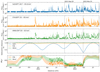 |
Fig. 1. Overview of multi-spacecraft near-relativistic electron observations made between 2020 February 28 and 2022 September 1. From top to bottom, the panels show ∼49.7 − 85.6 keV electron fluxes measured by Solar Orbiter/EPT, 55 − 85 keV electron fluxes measured by STEREO-A/SEPT, 50 − 82 keV electron fluxes measured by Wind/3DP, the heliocentric distance of all three spacecraft, and the longitudinal separation of the magnetic footpoints between Solar Orbiter and STEREO-A (orange) as well as between Solar Orbiter and Wind (green). The dots in the lowest panel show the separation angle approximated by using solar wind speed measurements from the different spacecraft, and the coloured areas show the minimum and maximum separation angle estimated for arbitrary solar wind speeds ranging from 300 to 500 km s−1. |
In this study, we specifically focused on the time period between the fourth and fifth perihelion of Solar Orbiter (September 2021–March 2022). This period is indicated in Fig. 1 by the vertical dashed lines. During this period, the orbit of Solar Orbiter enabled a particularly good connection to the other near 1 au spacecraft mentioned above. Within this time period, we identified all near-relativistic electron events that satisfied the following two selection criteria: (a) A clear flux increase of ∼50 − 85 keV electrons at Solar Orbiter and a clear flux increase of ∼50 − 85 keV electrons at either Wind, STEREO-A, or both; and (b) a longitudinal separation smaller than 15° of the nominal magnetic footpoints between Solar Orbiter and Wind or STEREO-A.
Following the criteria discussed above, we found 25 SEE events, which are listed in Tables 1 and 2. As in the 4 SEE events observed on 2022 January 16, January 18, February 13, and March 7, our selection criteria are satisfied by Wind and STEREO-A at the same time. These 4 events appear in both tables.
All selected SEE events with a small longitudinal separation between the magnetic footpoints of Solar Orbiter and STEREO-A.
All SEE events with a small longitudinal separation between the magnetic footpoints of Solar Orbiter and Wind.
To characterise the electron events, we determined a set of seven SEE event parameters: Onset time, slope of the early flux increase, separation angle of the magnetic foot-point, time of maximum, rise time, peak flux, and the first-order anisotropy. These parameters were determined for each electron event in our sample. Detailed descriptions of all parameters are given below.
3.1. Onset time
We approximated the arrival time of the first electrons of each SEE event at each spacecraft by determining the time when the ∼50 − 80 keV electron flux rose above the mean pre-event background plus three standard deviations. In particular, we used the following routine. (1) We calculated the moving mean  and moving standard deviation σi in a two-hour window from ti − 120 min, ti for the ∼55 − 80 keV electron flux. (2) We defined an onset at ti if two consecutive three-minute-averaged flux values rose by more than three standard deviations (
 and
and  ).
).
The 120-min background averages and the three-minute averages used here were assumed to provide a reasonable compromise between time resolution and statistical uncertainty. We note that the derived onset times we obtained following the process described above are only a rough estimate for the actual arrival time of the first electrons. The onset time found with the routine strongly depends on the instrument response, pre-event background, and pitch-angle coverage. In addition, gradual flux increases result in systematically delayed onset times because undetectable flux increases will raise the detection threshold.
3.2. Slope of the early flux increase
In order to describe how prompt a flux increase was after its onset, we determined the slope of the flux increase around the onset. We proceeded as follows. We determined the slope m = (I+9 min − I−3 min)/12 min in a [−3min, +9min] interval around the onset. I−3 min and I+9 min are three-minute-averaged omni-directional flux values observed three minutes before and nine minutes after the onset time.
We note that there is no general prediction of how exactly the flux increase develops around the onset. The increase rate is most likely not constant over time, and the slope derived in a 12-min-interval is therefore a somewhat arbitrary parameter. However, for the presented sample of events, this interval (3 min before the onset to 9 min after the onset) does not exceed the rise phase of any of the events in our sample. For shorter time intervals, the statistical uncertainties in the flux measurements would significantly increase the uncertainty in the slope parameter.
In this study, the estimated slope only serves as a simple assessment of how prompt the flux increase was, regardless of the observed peak flux.
3.3. Separation angle of the magnetic footpoints
For each event, we approximated the longitudinal separation angle between the magnetic footpoints of the spacecraft. We neglected the latitudinal separation of the magnetic footpoints because all spacecraft were close to the ecliptic plane (heliographic latitudes lower than ±5°) in the time period of interest. To determine the longitudinal magnetic footpoint separation angle, we used the following procedure. (1) We determined each spacecraft position at the time of the onset. (2) We determined the two-hour-averaged solar wind speed around the onset time at each spacecraft. (3) We calculated the longitudinal back-mapping angle β as β = ω⊙ ⋅ rspacecraft/vsw, where rspacecraft, vsw and ω⊙ are the radial distance of the spacecraft, the solar wind speed at the time of the onset, and the solar angular velocity for a sidereal rotation period of 25.38 days, respectively. (4) We calculated the longitudinal footpoint separation at the Sun ΔΦFP as the angle between the back-mapped longitudes ΦFP = Φ − β of the two spacecraft, where Φ is the longitude of the spacecraft, and β is the back-mapping angle.
We note that the separation angles were determined assuming an ideal Parker field and that significant deviations from this ideal scenario can occur, for example, due to the influence of interplanetary structures and the complex structure of the coronal magnetic field below the solar wind source surface.
3.4. Time of maximum and SEE peak flux
We determined the highest omni-directional (all-sector-averaged) flux values observed during each event together with the time when the maximum was reached. For this purpose, we used the following procedure. (1) We calculated 15-min running averages of the ∼55 − 80 keV electron flux. (2) We determined the highest value of the 15-min-averaged flux in an interval of [tonset, tonset + 300 min] after the SEE event onset. This value was then defined as the peak flux. (3) We determined the time when the highest 15-min-averaged flux was observed. This time was then taken as the time of maximum. (4) We defined the time between onset and time of maximum as the rise time.
By using 15-min-averages, we intended to reduce the statistical uncertainties. A similar timescale for the determination of peak intensities was used for example by Dresing et al. (2020). The 300-min window used as a limit to determine the time of maximum was introduced in order to prevent the method from detecting subsequent events. The specific value of 300 min was chosen after a visual inspection of the event sample. We note that the observed omni-directional peak flux and time of maximum depend on the exact pitch-angle coverage of the instrument. A further discussion of this aspect is given in Sect. 4.
3.5. Maximum first-order anisotropy
We used the sector intensities observed by the different instruments and the measurements of the local magnetic field vectors to calculate the peak value of the first-order anisotropy for each SEE event. We used the following procedure. (1) We calculated one-minute-averaged magnetic field vectors and sector intensities for each spacecraft. (2) For the four-sector measurements by STEREO-A/SEPT and Solar Orbiter/EPT, we estimated the first-order anisotropy A1 using the following equation:
 (1)
(1)
where I(μi), μi, and δμi are the observed intensities of sector i, the cosine of the pitch-angle of the central pointing axes of sector i, and the range in μ-space covered by sector i, respectively. Equation (1) was proposed by Brüdern et al. (2018) in order to reliably determine the first-order anisotropy in case of four-sector measurements. For Wind/3DP, we calculated the first-order anisotropy for eight-sector measurements by the following equation:
 (2)
(2)
where I(μi) and μi are the observed intensities of sector i and the pitch-angle of the inverted central pointing axes of sector i, respectively. The first-order anisotropy for Wind was calculated without considering the actual pitch-angle coverage of the individual sectors δμi because the exact coverage could not be identified. (3) We calculated a three-minute moving average of the first-order anisotropy and determined its highest value. This value was then selected as the maximum first-order anisotropy. We note that the maximum value of the anisotropy observed also depends on the exact pitch-angle coverage of the instrument. Again, this is further discussed in Sect. 4.
4. Analysis
We analysed the event parameters derived from the 25 near-relativistic SEE events listed in Tables 1 and 2. For each SEE event, the date of the observation is given in the first column, and the next three columns of the tables list the spacecraft position in Stonyhurst coordinates. The radial distance, R (1), is given in astronomical units; the longitude, Φ (2), and latitude, Θ (3), are given in degrees. The onset time, tonset (4), and the time at which the peak flux was observed, tImax (6), are given with an approximate uncertainty of ±3 min, which was estimated based on the time averages used here. The peak flux, Imax (5), is given in units of electrons per (cm2 sr s MeV). The solar wind speed, vsw (7), at the time of the onset is given in km s−1. The maximum values of the first-order anisotropy,  (8), are unitless. The slope of the flux increase around the onset, m (9), is given in units of electrons per (cm2 sr s2 MeV). The separation angle between the magnetic footpoints at the Sun, ΔΦFP (10), is given in degrees. The last Col. (11) indicates whether a significant flux increase was observed at all three spacecraft.
If no value for the first-order anisotropy is given, the parameter could not be determined due to lack of magnetic field data. For four SEE events, indicated with an (a) in the table, no solar wind data were available from Solar Orbiter around the onset of the event. In this case, we used the nearest observed solar wind speed for the back-mapping. Figure 2 shows an example of the determined event parameters and the corresponding observations for the event observed on 2022 March 19.
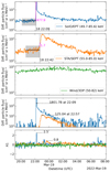 |
Fig. 2. Time profiles used to determine the event parameters shown for the event observed on 2022 March 18. From top to bottom: near-relativistic electron fluxes observed by Solar Orbiter/EPT (heliocentric distance of 0.36 AU at 22:09 UT on March 18), STEREO-A/SEPT (heliocentric distance of 0.97 AU at 22:42 UT on March 18), and Wind/3DP, the background-subtracted fluxes, and the first-order anisotropy. The black lines and grey areas in the first two panels identify the mean of the pre-event background and the ±3σ levels. The dotted lines identify the onset times. The values in the fourth panel are the 15-min-averaged background-subtracted peak fluxes. The values in the bottom panel are three-minute-averaged values of the maximum first-order anisotropy. |
In four SEE events, our selection criteria presented in Sect. 3 were satisfied by STEREO-A and Wind simultaneously, meaning that all three spacecraft presented close nominal magnetic footpoint locations. For the 29 pairs of observation points (Tables 1 and 2 together), we analysed the event parameters in terms of their radial gradients. In particular, we determined the gradient of the peak intensity, first-order anisotropy, slope of the early flux increase, and rise time. Figure 3 shows a summary of the event parameters vs. the radial distance for each spacecraft.
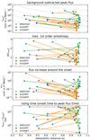 |
Fig. 3. Radial dependence of the peak intensity, maximum first-order anisotropy, flux increase around the onset, and the time to maximum. Observations made by Solar Orbiter/EPT, Wind/3DP, and STEREO-A/SEPT are shown as blue circles, green triangles, and orange squares, respectively. The solid lines connect observations of the same event. The line colours correspond to the marker colours of the 1 au spacecraft. The dotted lines in the top panel show a dependence on I ∝ R−3. |
Following former studies such as Rodríguez-García et al. (2023) and theoretical considerations (e.g., given by Vainio et al. 2007), we characterised the radial gradient of the omni-directional peak intensity by the exponential index αI, given by
 (3)
(3)
where I1 and I2 are the peak intensities observed at the two spacecraft, and R1 and R2 are the corresponding radial distances of the spacecraft. For the other SEE event parameters, we determined the exponential indices in an analogous way, in order to characterise the radial gradients of the first-order anisotropy (αA), the slope of the early flux increase (αm), and the rise time (αT). The exponential indices derived from the 25 SEE events for the different parameters analysed here are listed in Tables 3 and 4.
Exponential indices for the radial gradients in the event parameters observed by STEREO-A and Solar Orbiter.
Exponential indices for the radial gradients in the event parameters observed by Wind and Solar Orbiter.
Because of the various uncertainties in the event parameters discussed in Sects. 3 and 5, small changes in event parameters over short radial distances cannot be resolved by our analysis. Therefore, we restricted our further analysis to events for which the radial distance between the spacecraft was greater than 0.1 au. The remaining events are still affected by the same uncertainties, but the same errors ΔI1 and ΔI2 of the parameters I1 and I2 will yield a smaller error ΔαI of the gradient αI at larger radial separations. Following the error propagation of Eq. (3) and neglecting the errors of the spacecraft positions, the error of the gradient is given by
 (4)
(4)
Although no exact values for ΔI1 and ΔI2 could be determined here, Eq. (4) shows that the error ΔαI becomes increasingly larger for decreasing radial separations as log(R1/R2) approaches zero.
In 17 out of 25 SEE events, Solar Orbiter had a radial distance ≥0.1 au with respect to the other spacecraft. In 2 of these 17 events, STEREO-A and Wind satisfied our selection criteria simultaneously. For the total of 19 pairs of observations, we found 15 cases in which the peak intensity decreases with increasing radial distance. In 8 out of 15 cases in which we were able to determine the first-order anisotropy, the maximum value of the anisotropy decreases with increasing radial distance. The slope of the early flux increase decreases in 17 out of 19 cases, and the rise time increases in 10 out of 19 cases.
In the SEE event on 2022 February 13, the gradients αI, αA1, and αm determined between Solar Orbiter (R = 0.77 au) and Wind (R = 0.99 au) contradict the corresponding gradients derived for the same event between Solar Orbiter and STEREO-A (R = 0.97 au). During the SEE event, Wind observed the highest fluxes and first-order anisotropy, followed by Solar Orbiter. The lowest fluxes and first-order anisotropy were observed by STEREO-A. This SEE event is also one of the cases for which no solar wind speed measurement was available for Solar Orbiter. The footpoint separation was estimated with a solar wind speed of 306 km s−1. The estimated longitudinal separation angles were +4.9° between Solar Orbiter and Wind and −13.7° between Solar Orbiter and STEREO-A.
An unambiguous identification of the solar source was not possible for this event. However, one potential candidate is the class C6.2 flare that appeared at the NOAA active region AR12941 around 01:47 UT, located N29W38 as seen from Earth. When we assume that this is the actual source, Wind would have the closest longitudinal connection to the source, followed by Solar Orbiter, while STEREO-A would have the largest longitudinal separation to the source. In this constellation, perpendicular transport might be the dominant process that effects the SEE event parameter here. Even though we limited our sample to events where the estimated footpoints were closely spaced, the 2022 February 13 event indicates that the actual source separation still plays a significant role. Further discussion of the influence of the source separation can be found in Rodríguez-García et al. (2023).
A clear identification of the source location for all events considered here is beyond the scope of this study. For future studies, a selection of events that are well connected to the source might reduce the influence of longitudinal transport effects, and radial dependences would likely become more prominent.
In addition to the four parameters discussed above, we also compared the timing of the electron arrival at the different spacecraft. We performed this analysis with the full sample of events, including events with dR < 0.1 au. Figure 4 shows the difference in the onset times versus the heliocentric distance between the spacecraft, together with estimates for the onset delays, assuming that all particles travel along an ideal Parker spiral. For the estimates, we assumed a solar wind speed of 250 km s−1 and arbitrarily chosen pitch-angles from 0° to 89°. These estimates are intended to represent extreme cases for particularly long path lengths along an ideal Parker spiral. We calculated the delay of ideal propagating particles, T, by
 (5)
(5)
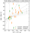 |
Fig. 4. Timing difference between the onsets observed by Solar Orbiter and STEREO-A/Wind vs. the difference in their radial distance. The dotted line shows the ideal travel time for radially propagating 55 keV electrons. The solid lines show the ideal travel time assuming the electrons travel along a Parker spiral (vsw = 250 km s−1), with various constant pitch-angles ranging from of 0° to 89°. |
where L is the Parker spiral length between Solar Orbiter and a spacecraft located at 1 au, α is the pitch-angle, c is the speed of light, m0 is the electron rest mass, and E is the kinetic energy.
For our sample, the majority of events show onset delays that are significantly larger than the expected delays for particles propagating along an ideal Parker spiral. Even when we assume that all observed particles maintained an arbitrary pitch-angle of 70°, the observed onset delays are too long. In five events, we found onset delays > 40 min between the spacecraft. With a relativistic speed of ∼0.52 au min−1 for 55 keV electrons, these delays would correspond to path lengths > 2 au. The exact cause for the long onset delays cannot be determined with certainty here.
A comparison of the ratio of the peak intensities at the different spacecraft with the onset delays in each event is shown in Fig. 5. The clear correlation between these two quantities might be an indication for the systematic errors introduced by the procedure used to determine the onsets. The smaller the flux increase, the longer the time the flux needs to emerge from the pre-event background to become detectable. For the majority of events, the outer spacecraft observed a significantly smaller flux increase than the inner spacecraft. Therefore, the systematic error in the onset detection at the outer spacecraft would often be greater. Larger errors at the outer spacecraft directly translate into an increased delay between the onsets that are detected at the two spacecraft. A critical discussion of the use of the onset determination method is given in the discussion.
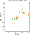 |
Fig. 5. Onset delay observed between Solar Orbiter and STEREO-A (orange) and Solar Orbiter and Wind (green) vs. the ratio of the observed peak fluxes. |
5. Summary and discussion
We have analysed 25 near-relativistic electron events that were observed by Solar Orbiter EPD/EPT in the time between the fourth and fifth perihelion of Solar Orbiter. Our selection included only events that were also observed by Wind/3DP or STEREO-A/SEPT. We further limited the sample to events for which the different spacecraft featured a similar magnetic connection to the Sun, where the nominal magnetic footpoints of the spacecraft were separated by less than 15 deg in longitude.
For the given event sample, we determined a set of SEE event parameters using routines that are well established in the energetic particle community. These parameters include the onset time of the flux increase, the slope of the early flux increase, the peak flux and time of maximum, and the maximum value of the first-order anisotropy. Comparing the event parameters derived for the same SEE event by different observers at different locations, we find a wide variability in the SEE parameters and their corresponding gradients in radial direction.
A statistical evaluation of the SEE parameters with respect to their radial dependences shows the following tendencies: In 15 out of 17 cases, the peak intensity decreases with increasing radial distance. The maximum value of the first-order anisotropy decreases in 8 out of 15 cases with increasing radial distance. The slope of the early flux increase decreases in 17 out of 19 cases, and the rise time increases in 10 out of 19 cases with increasing radial distance.
Comparing the relative onset times of electrons at the different spacecraft, we again find a wide variability. For the majority of events, the derived delays are significantly larger than estimates based on ideal Parker spirals. The derived onset delays also show a correlation with the ratio of the peak intensities between the two spacecraft.
The long onset delays and the absence of clear radial dependences in the first-order anisotropy and the rise time point to limitations of the analysis methods. The rudimentary approaches for determining event parameters chosen in this study are most likely insufficient to accurately characterise the radial evolution of SEE events.
For example, the assumption of an ideal Parker field is not generally valid, and the complexity of the coronal magnetic field was not considered here. The deviation of our estimates from the real magnetic footpoints could be one crucial driver for the large variability in the radial gradients we found. In addition, all parameters used here are strongly dependent on the exact instrument response. The sensitivity and background of the different instruments influence, for example, how fast a certain flux increase can be detected (e.g., Laitinen et al. 2015). The different instruments also have unique directional particle acceptances that directly translate into different pitch-angle coverage and pitch-angle responses. The observed peak intensity, the slope of the early flux increase, and the observed anisotropy will depend on these directional responses. For instance, an unfavourable pitch-angle coverage, for which none of the EPT telescopes looks along the magnetic field, could lead to the observation of a low peak intensity and low anisotropy because the instrument looked past an ambient particle beam.
The strong changes in the event parameters and the enormous gradients (|α|> 10) observed in events where Solar Orbiter had a small radial separation (ΔR < 0.1 au) from the other spacecraft are a finding that particularly requires discussion. For spacecraft that supposedly have a similar magnetic connection to the Sun and about the same radial distance, we expected minor changes in the event parameters. In contradiction to this, we find events with extremely large indices at these constellations in our sample (e.g., the SEE events on 2022 January 20 and 2022 January 30). For these unexpected observations, we consider two possible explanations here.
First, the instrumental differences mentioned above might affect the results. In our study, we used sector-averaged fluxes as an estimate for the pitch-angle-averaged (omni-directional) flux. However, the sectors of EPT, SEPT, and 3DP usually cover different pitch-angle ranges. We note that in particular the sectors of SEPT have a different pointing than the sectors of EPT because the STEREO-A spacecraft was rolled during its solar superior conjunction (from January to August 2015). Furthermore, the exact pitch-angle response will differ between the instruments. Thus, the sector-averaged fluxes from the three instruments are averages over different limited pitch-angle ranges with individual weights. During anisotropic time periods, these different averages are not directly comparable (e.g., Fig. 6 by Bruedern et al. 2022). The sector averages used in this study can only be used as a rough estimate for the full 180° pitch-angle-averaged flux. This limitation will not only affect peak intensities, but also increase the times and the slope of the flux increase observed around the onset. In addition, the maximum anisotropy that can be observed will also depend on the exact pitch-angle coverage of the instruments (e.g., Bruedern et al. 2022). The large differences in the event parameters between the observations of Wind/3DP and Solar Orbiter/EPT observations during Solar Orbiter EGAM (events around December 2021 to January 2021) are another indication of the limited comparability of the event parameters derived from the sector-averaged (omni-directional) intensities. The differences in the individual events are currently under investigation, and their interpretation is beyond the scope of this work. Detailed event studies as well as a cross validation of the instrument calibrations will be needed in order to understand and explain the observed differences. A discussion of how sufficiently the inter-calibration can affect the derived radial gradients of the peak intensity can be found in Rodríguez-García et al. (2023). For all events with significant anisotropies, a comparison of pitch-angle-dependent intensities would clearly be more suitable. A detailed analysis of the pitch-angle coverage and the pitch-angle response of each instrument would most likely increase the precision of our analysis. However, an analysis like this was beyond the scope of this study, and the essential magnetic field data necessary for a pitch-angle-dependent study were not available for several events.
Second, the interplanetary context is a possible explanation for some differences. For events for which two spacecraft are located in flux tubes that are similarly situated but different, any differences in the event parameters might be observed despite the small spacecraft separation. An example for this type of observation was reported by Klassen et al. (2016) and was further analysed by Pacheco et al. (2017).
Further studies are needed to take all these effects into account. In particular, simulations of the individual events that take into account the exact instrument responses would help to separate the instrumental influence and the actual influence of the involved transport processes on the observations. The benefits of this approach are for example shown in Agueda et al. (2008).
For the long onset delays found in this study, we consider the following three possible explanations.
First, the actual path lengths might be significantly longer than those estimated by a Parker spiral. This might be the case if the magnetic footpoints are subject to strong meandering, for example (e.g., Laitinen & Dalla 2019). In this case, the estimated magnetic footpoints would also be affected because the intrinsic assumption of an ideal Parker field would not be fulfilled.
Second, if the electrons are subject to substantial scattering between the observers, a longer onset delay might be expected. If almost none of the electrons propagate scatter free, there is no meaningful definition of a path length.
Third, the method for determining the onsets has well-known limitations (see e.g., Saiz et al. 2005; Laitinen et al. 2015). For small and/or gradual flux increases, the procedure often yields times that are significantly delayed with respect to the arrival time of the first particles, and high pre-event backgrounds will lead to even longer delays. The correlation of the onset delay with the ratio of the peak fluxes shown in Fig. 5 is an indication for such a systematic uncertainty.
The limitations of the onset determination method we used mean that it is highly questionable whether this simple method is sufficient to resolve timing differences of several minutes. For further analysis, we suggest an evaluation of the pitch-angle dependent fluxes to determine the onset times, as well as a detailed comparison of the detection thresholds of the different instruments.
In conclusion, this study presents a series of near-relativistic electron events and shows the wide event-to-event variability in the radial dependence of commonly used SEE event parameters. As a possible explanation for the wide variability, we specifically pointed out the limitations of the parameters and described the potential shortcomings in the methods we used to derive these parameters. For future studies of the radial evolution of SEE events, we recommend to consider pitch-angle dependent fluxes in order to overcome some of the critical problems with the parameters we used here.
Acknowledgments
Solar Orbiter is a mission of international cooperation between ESA and NASA, operated by ESA. This work was supported by the German Space Agency (Deutsches Zentrum für Luft- und Raumfahrt, e.V., (DLR)) under grant number 50OT2002. N.D. is grateful for support by the Academy of Finland (SHOCKSEE, grant no. 346902). This work received funding from the European Union’s Horizon 2020 research and innovation program under grant agreement No. 101004159 (SERPENTINE). The UAH team acknowledges the financial support by the Spanish Ministerio de Ciencia, Innovación y Universidades FEDER/MCIU/AEI Projects ESP2017-88436-R and PID2019-104863RB-I00/AEI/10.13039/501100011033.
References
- Acuña, M., Ogilvie, K., Baker, D., et al. 1995, Space Sci. Rev., 71, 5 [CrossRef] [Google Scholar]
- Acuña, M. H., Curtis, D., Scheifele, J. L., et al. 2008, Space Sci. Rev., 136, 203 [Google Scholar]
- Agueda, N., Vainio, R., Lario, D., & Sanahuja, B. 2008, ApJ, 675, 1601 [NASA ADS] [CrossRef] [Google Scholar]
- Agueda, N., Lario, D., Vainio, R., et al. 2009, A&A, 507, 981 [NASA ADS] [CrossRef] [EDP Sciences] [Google Scholar]
- Brüdern, M., Dresing, N., Heber, B., et al. 2018, Cent. Eur. Astrophys. Bull., 42, 2 [Google Scholar]
- Bruedern, M., Berger, L., Heber, B., et al. 2022, in 44th COSPAR Scientific Assembly. Held 16–24 July, 44, 1298 [Google Scholar]
- Domingo, V., Fleck, B., & Poland, A. I. 1995, Sol. Phys., 162, 1 [Google Scholar]
- Dresing, N., Effenberger, F., Gómez-Herrero, R., et al. 2020, ApJ, 889, 143 [NASA ADS] [CrossRef] [Google Scholar]
- Dröge, W., Kartavykh, Y. Y., Klecker, B., & Kovaltsov, G. A. 2010, ApJ, 709, 912 [CrossRef] [Google Scholar]
- Dröge, W., Kartavykh, Y. Y., Dresing, N., & Klassen, A. 2016, ApJ, 826, 134 [Google Scholar]
- Fox, N. J., Velli, M. C., Bale, S. D., et al. 2016, Space Sci. Rev., 204, 7 [Google Scholar]
- Galvin, A. B., Kistler, L. M., Popecki, M. A., et al. 2008, Space Sci. Rev., 136, 437 [Google Scholar]
- He, H.-Q., & Wan, W. 2012, ApJ, 747, 38 [NASA ADS] [CrossRef] [Google Scholar]
- Horbury, T. S., Obrien, H., Carrasco Blazquez, I., et al. 2020, A&A, 642, A9 [NASA ADS] [CrossRef] [EDP Sciences] [Google Scholar]
- Jokipii, J. R. 1966, ApJ, 146, 480 [Google Scholar]
- Klassen, A., Dresing, N., Gómez-Herrero, R., Heber, B., & Müller-Mellin, R. 2016, A&A, 593, A31 [NASA ADS] [CrossRef] [EDP Sciences] [Google Scholar]
- Laitinen, T., & Dalla, S. 2019, ApJ, 887, 222 [Google Scholar]
- Laitinen, T., Huttunen-Heikinmaa, K., Valtonen, E., & Dalla, S. 2015, ApJ, 806, 114 [Google Scholar]
- Lepping, R. P., Acũna, M. H., Burlaga, L. F., et al. 1995, Space Sci. Rev., 71, 207 [Google Scholar]
- Lin, R. P., Anderson, K. A., Ashford, S., et al. 1995, Space Sci. Rev., 71, 125 [CrossRef] [Google Scholar]
- Mueller-Mellin, R., Green, G., Iwers, B., et al. 1982, Data Processing for a Cosmic ray Experiment Onboard the Solar Probes HELIOS 1 and 2: Experiment 6, Final Report, Oct. 1981 Kiel Univ. (Germany). Inst. für Reine und Angewandte Kernphysik [Google Scholar]
- Müller, D., St Cyr, O. C., Zouganelis, I., et al. 2020, A&A, 642, A1 [Google Scholar]
- Müller-Mellin, R., Böttcher, S., Falenski, J., et al. 2008, Space Sci. Rev., 136, 363 [Google Scholar]
- Ogilvie, K. W., Chornay, D. J., Fritzenreiter, R. J., et al. 1995, Space Sci. Rev., 71, 55 [Google Scholar]
- Owen, C. J., Bruno, R., Livi, S., et al. 2020, A&A, 642, A16 [EDP Sciences] [Google Scholar]
- Pacheco, D., Agueda, N., Gómez-Herrero, R., & Aran, A. 2017, J. Space Weather Space Clim., 7, A30 [NASA ADS] [CrossRef] [EDP Sciences] [Google Scholar]
- Rodríguez-Pacheco, J., Wimmer-Schweingruber, R. F., Mason, G. M., et al. 2020, A&A, 642, A7 [Google Scholar]
- Rodríguez-García, L., Gómez-Herrero, R., Dresing, N., et al. 2023, A&A, 670, A51 (SO Nominal Mission Phase SI) [NASA ADS] [CrossRef] [EDP Sciences] [Google Scholar]
- Russell, C. T. 2008, The STEREO Mission (New York: Springer) [CrossRef] [Google Scholar]
- Saiz, A., Evenson, P., Ruffolo, D., & Bieber, J. W. 2005, ApJ, 626, 1131 [CrossRef] [Google Scholar]
- SEPT Online Event List 2022, STEREO Electron Event List [Google Scholar]
- Strauss, R. D., & Fichtner, H. 2015, ApJ, 801, 29 [NASA ADS] [CrossRef] [Google Scholar]
- Strauss, R. D. T., Dresing, N., & Engelbrecht, N. E. 2017, ApJ, 837, 43 [NASA ADS] [CrossRef] [Google Scholar]
- Vainio, R., Agueda, N., Aran, A., & Lario, D. 2007, in Space Weather: Research Towards Applications in Europe 2nd European Space Weather Week (ESWW2), ed. J. Lilensten, Astrophys. Space Sci. Lib., 344, 27 [CrossRef] [Google Scholar]
- Wenzel, K. P., Marsden, R. G., Page, D. E., & Smith, E. J. 1992, A&AS, 92, 207 [Google Scholar]
- Wibberenz, G., & Cane, H. V. 2006, ApJ, 650, 1199 [NASA ADS] [CrossRef] [Google Scholar]
- Wibberenz, G., Kecskeméty, K., Kunow, H., et al. 1989, Sol. Phys., 124, 353 [NASA ADS] [CrossRef] [Google Scholar]
All Tables
All selected SEE events with a small longitudinal separation between the magnetic footpoints of Solar Orbiter and STEREO-A.
All SEE events with a small longitudinal separation between the magnetic footpoints of Solar Orbiter and Wind.
Exponential indices for the radial gradients in the event parameters observed by STEREO-A and Solar Orbiter.
Exponential indices for the radial gradients in the event parameters observed by Wind and Solar Orbiter.
All Figures
|
Fig. 1. Overview of multi-spacecraft near-relativistic electron observations made between 2020 February 28 and 2022 September 1. From top to bottom, the panels show ∼49.7 − 85.6 keV electron fluxes measured by Solar Orbiter/EPT, 55 − 85 keV electron fluxes measured by STEREO-A/SEPT, 50 − 82 keV electron fluxes measured by Wind/3DP, the heliocentric distance of all three spacecraft, and the longitudinal separation of the magnetic footpoints between Solar Orbiter and STEREO-A (orange) as well as between Solar Orbiter and Wind (green). The dots in the lowest panel show the separation angle approximated by using solar wind speed measurements from the different spacecraft, and the coloured areas show the minimum and maximum separation angle estimated for arbitrary solar wind speeds ranging from 300 to 500 km s−1. |
| In the text | |
|
Fig. 2. Time profiles used to determine the event parameters shown for the event observed on 2022 March 18. From top to bottom: near-relativistic electron fluxes observed by Solar Orbiter/EPT (heliocentric distance of 0.36 AU at 22:09 UT on March 18), STEREO-A/SEPT (heliocentric distance of 0.97 AU at 22:42 UT on March 18), and Wind/3DP, the background-subtracted fluxes, and the first-order anisotropy. The black lines and grey areas in the first two panels identify the mean of the pre-event background and the ±3σ levels. The dotted lines identify the onset times. The values in the fourth panel are the 15-min-averaged background-subtracted peak fluxes. The values in the bottom panel are three-minute-averaged values of the maximum first-order anisotropy. |
| In the text | |
|
Fig. 3. Radial dependence of the peak intensity, maximum first-order anisotropy, flux increase around the onset, and the time to maximum. Observations made by Solar Orbiter/EPT, Wind/3DP, and STEREO-A/SEPT are shown as blue circles, green triangles, and orange squares, respectively. The solid lines connect observations of the same event. The line colours correspond to the marker colours of the 1 au spacecraft. The dotted lines in the top panel show a dependence on I ∝ R−3. |
| In the text | |
|
Fig. 4. Timing difference between the onsets observed by Solar Orbiter and STEREO-A/Wind vs. the difference in their radial distance. The dotted line shows the ideal travel time for radially propagating 55 keV electrons. The solid lines show the ideal travel time assuming the electrons travel along a Parker spiral (vsw = 250 km s−1), with various constant pitch-angles ranging from of 0° to 89°. |
| In the text | |
|
Fig. 5. Onset delay observed between Solar Orbiter and STEREO-A (orange) and Solar Orbiter and Wind (green) vs. the ratio of the observed peak fluxes. |
| In the text | |
Current usage metrics show cumulative count of Article Views (full-text article views including HTML views, PDF and ePub downloads, according to the available data) and Abstracts Views on Vision4Press platform.
Data correspond to usage on the plateform after 2015. The current usage metrics is available 48-96 hours after online publication and is updated daily on week days.
Initial download of the metrics may take a while.