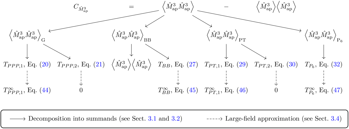
Schematic representation of the calculation of the covariance . The covariance is given by the difference between and , the first of which can be decomposed (indicated by solid arrows) into one Gaussian (denoted by G) and three non-Gaussian parts (denoted by BB, PT, and P₆). We discuss the Gaussian part in Sect. 3.1 and the non-Gaussian parts in Sect. 3.2. These parts can be further decomposed into terms depending on different permutations of the aperture scale radii, called T_PPP, 1 to T_P6. For large survey areas, the T_i can be approximated, indicated by dashed arrows, as shown in Sect. 3.4. Under this approximation, two terms vanish, which is why we term them ‘finite-field terms’. Also shown are equation numbers for the relevant expressions.