| Issue |
A&A
Volume 670, February 2023
|
|
|---|---|---|
| Article Number | A40 | |
| Number of page(s) | 13 | |
| Section | Stellar structure and evolution | |
| DOI | https://doi.org/10.1051/0004-6361/202244926 | |
| Published online | 02 February 2023 | |
Fictitious neutron sinks to trace radiative s-process nucleosynthesis
Institut d’Astronomie et d’Astrophysique (IAA), Université Libre de Bruxelles (ULB), CP226, Boulevard du Triomphe, 1050 Brussels, Belgium
e-mail: pawel.krynski@ulb.be
Received:
8
September
2022
Accepted:
29
November
2022
Context. Asymptotic giant branch (AGB) stars are strong producers of s-process elements, which are synthesized by successive slow neutron captures on elements heavier than iron. The nucleosynthesis calculation involves solving large nuclear networks with hundreds of nuclei, which in a stellar evolution code can greatly extend the computational time. However, the s-process is often measured using a handful of elements located on the neutron magic shells and grouped into tracers called ls, hs, and vhs.
Aims. We propose a fictitious network that approximates the production of ls, hs, and vhs species at a minimal computational expense. The network is specifically designed for the radiative s-process in AGB stars. It is an alternative to methods using large networks that can be used as a fast exploratory tool to trace the production of s-elements.
Methods. The fictitious network was constructed by assembling species with Z ≥ 18 into seven fictitious particles whose abundances and reaction rates model the effective properties of the corresponding groups. The effective reaction rates were tabulated as a function of neutron density and number of neutrons captured per initial heavy seed (Ncapt) using single-zone nucleosynthesis calculations. The accuracy of our network was tested by comparing the abundances obtained with the fictitious and large networks during the radiative burning of 13C during the interpulse period of a 2 M⊙, [Fe/H] = −2 star.
Results. The fictitious network reliably reproduces the abundances of ls, hs, and vhs species during the radiative s-process. The accuracy of the method increases with the strength of the nucleosynthesis as measured by Ncapt, but diminishes when the nuclear distribution is different from the initial distribution. This network is well suited to follow the s-process nucleosynthesis in low-mass AGB stars where neutrons are mainly produced below the envelope by the 13C(α, n) reaction.
Key words: nuclear reactions / nucleosynthesis / abundances / stars: AGB and post-AGB / methods: numerical
© The Authors 2023
 Open Access article, published by EDP Sciences, under the terms of the Creative Commons Attribution License (https://creativecommons.org/licenses/by/4.0), which permits unrestricted use, distribution, and reproduction in any medium, provided the original work is properly cited.
This article is published in open access under the Subscribe-to-Open model. Subscribe to A&A to support open access publication.
1. Introduction
The slow neutron-capture process (s-process) is thought to be responsible for about half of the abundances of trans-iron elements in the Galaxy (Arlandini et al. 1999). It occurs in stellar interior, where preexisting seed nuclei capture neutrons, forming heavier isotopes until they become unstable and decay through the β− channel. The process is defined as slow in the sense that most β− decays occur faster than neutron captures, which forces the nucleosynthetic path to follow the valley of β-stability in the table of nuclides. It is associated with low neutron densities ranging from ∼107 to 1012 cm−3. With higher neutron densities, branching points open up and slightly modify the path taken by the s-process. This affects the production of specific isotopes such as 96Mo or 142Nd (e.g., Bisterzo et al. 2015). The s-process nucleosynthesis stops at 209Bi, after which the chain of reactions 209Bi(n, γ) 210Bi(β+) 210Po(γ, α) 206Pb closes the cycle. The s-process has two main components (Kappeler et al. 1989). The weak component includes elements with atomic number 70 ≤ A ≤ 90 and takes place in the late stages of core helium burning of massive stars. There, neutrons are provided by the reaction 22Ne(α, n) 25Mg (Langer et al. 1989). The main component synthesizes nuclei with 90 ≤ A ≤ 204 and occurs in low- and intermediate-mass stars (between 1 and 8 M⊙) during their late evolutionary stages, which is called asymptotic giant branch (AGB; Herwig 2005; Goriely & Siess 2005; Cristallo et al. 2011; Karakas & Lattanzio 2014). In AGB stars, neutrons are produced by the reaction 13C(α, n) 16O (Straniero et al. 1995; Neyskens et al. 2015), although 22Ne(α, n) 25Mg can also be activated in the thermal pulse of massive AGB stars with mass M ≳ 2 M⊙ (Lugaro et al. 2012).
In an AGB star, the production of the neutron source starts during the third dredge-up (3DU) when protons from the H-rich convective envelope mix with the underlying 12C radiative layer. There, proton captures on 12C lead to the formation of the 13C pocket, which provides the source of neutrons during the interpulse phase. The neutron densities attained through the 13C(α, n) reaction are relatively low (≲ 108 cm−3), yet the main component elements can be produced due to the long neutron exposure. The mass of the 13C pocket, hence the efficiency of the s-process, depends on the mixing mechanism by which protons are transported below the envelope. Various processes have been invoked; among them, convective overshooting (Goriely & Mowlavi 2000), rotational mixing (Herwig 2005; Cristallo et al. 2011), gravitational waves (Denissenkov & Tout 2003), or mixing induced by magnetic fields (Nucci & Busso 2014; Trippella et al. 2016; Vescovi et al. 2020).
The s-process elements are often grouped into three categories depending on their mass: light (ls), heavy (hs), and very heavy (vhs) species. They are bounded by nuclei with magic neutron numbers (N = 50, 82, 126), which are characterized by small neutron-capture cross sections. They thus act as bottlenecks in the s-process and present enhanced abundances. The relative abundances of the peak elements are often used to measure the efficiency of the s-process (e.g., Cristallo et al. 2011).
It can become computationally expensive to follow the detailed s-process nucleosynthesis during the AGB phase. The traditional approach has therefore been to use a small nuclear network of 10–50 species to accurately follow the energetics of the star and then post-process the stellar models using an extended network of ≥400 species (e.g., Lugaro et al. 2012; Gil-Pons et al. 2021; Herwig et al. 2003; Battino et al. 2019; Campbell & Lattanzio 2008).
To account for the neutron captures on the heavy species that are not present in the energy network, Jorissen & Arnould (1989) introduced a fictitious particle called the heavy neutron sink. This particle models the effective properties of all species that are removed from the extended network. With the production of heavier nuclei with a large neutron cross section, the effective neutron capture changes as well. This effect was modeled in Jorissen & Arnould (1989) by performing nucleosynthesis calculations on a single zone using physical conditions representative of the s-process and calculating the effective cross section of the heavy sink as a function of the neutron exposition. The heavy neutron sink approach was subsequently used in numerous stellar evolution codes with satisfactory effects on the neutron density (Forestini et al. 1992; Herwig et al. 2003; Karakas & Lattanzio 2003; Cruz et al. 2013; Gil-Pons et al. 2021).
The aim of this work is to improve the neutron sink approach introduced in Jorissen & Arnould (1989) by considering seven additional fictitious particles to trace the abundances of the ls, hs, and vhs species. In this way, we can approximately follow the efficiency of the s-process using a small nuclear network at a minimal expense in computational complexity. We also improve the method used in Jorissen & Arnould (1989) by tabulating the effective capture cross sections as a function of neutron density and neutrons captured per initial heavy seed instead of neutron exposure. This provides a more physical interpolation of the cross sections to variable physical conditions that may impact the branching points of the s-process.
The paper is organized as follows. Section 2 is devoted to the description of the formalism of the fictitious network. In Sect. 3, we perform the one-zone simulations we used to tabulate the effective cross sections of the fictitious particles. Section 4 analyzes the radiative s-process using our fictitious network using the stellar evolution code STAREVOL. Finally, conclusions are drawn in Sect. 5.
2. Formalism of fictitious particles
2.1. Defining the fictitious particles
Our goal is to reduce an extended network including 1160 species and 2125 reactions to a minimum network capable of mimicking the s-process nucleosynthesis. This network is referred to as the large network, and its details can be found in Goriely & Siess (2018) and Choplin et al. (2021). The reduction was made by grouping real nuclei with Zi > ZCl into fictitious particles whose physical properties mirror the properties of the entire set. The nuclei with Zi ≤ ZCl and their reactions are part of our default AGB network that is used to determine the energetics and follow the abundances of the light elements. It is composed of 54 elements up to 37Cl and a fictitious neutron sink coupled through 168 reactions as described in Siess & Arnould (2008) and is referred to as the energy network.
Each fictitious particle k is defined by a couple of mass numbers (Ak, min; Ak, max) such that it contains all nuclei i with atomic mass number Ak, min ≤ Ai ≤ Ak, max. Because the groups are delineated along isobars, unstable species and the products of their decay remain in the same fictitious group. This is crucial to our reduced network, as it implies that the abundances of fictitious particles are not affected by β− decays and are effectively stable.
Three of the fictitious particles that trace the s-process elements (ls, hs, and vhs) were constructed such that they contain the stable species with the same magic neutron numbers (N = 50, 82 and 126, respectively) and all of their isobars. Owing to their small neutron-capture cross sections, they act as bottlenecks for the s-process, and their abundance is greatly enhanced compared to other elements. As an example, the ls fictitious particle is composed of stable nuclei with N = 50, namely 86Kr, 87Rb, 88Sr, 89Y, and 90Zr, plus all the other nuclei with mass number between Als, min = 86 and Als, max = 90. This adds the nuclei 86Sr, 87Sr, 89Sr, 90Sr 86Rb, and 90Y to the ls group. For vhs, we also included all elements involved in the Pb recycling process, so that this fictitious particle effectively plays the role of the end point of the s-process.
The nuclei in between the ls and hs form the lse particle and are bounded by 91 ≤ Ai ≤ 136, while those between hs and vhs form the hse particle and have 143 ≤ Ai ≤ 205. The nuclei with 56 ≤ Ai ≤ 85 form the fictitious particle fe. At the start of the s-process, this group is essentially dominated by the abundant 56Fe. Finally, the particle light connects the energy and fictitious parts of our network and is an exception to the isobar criterion as it contains nuclei with Zi > ZCl and Ai ≤ 55. The specific condition on Zi allowed us to keep all chlorine isotopes in the energy network.
Our large network also contains reactions that bring back nuclei from the light group to the energy network: 37Ar(n, p) 37Cl, 37Ar(e−, νe) 37Cl,37Ar(n, α)34S,39Ar(n, α) 36S, and 40K(n, α) 37Cl. We have verified in our simulations that neglecting these reactions has very limited effects on the abundance of the light particle and almost none on the abundances of the heavier fictitious groups. When these reactions are neglected in the fictitious network, only neutron captures affect the abundances of the fictitious particles. The definition of the fictitious particles is summarized in Table 1.
Fictitious particles are constructed by grouping nuclei with atomic mass number Ak, min ≤ Ai ≤ Ak, max.
Before defining the physical properties of the fictitious particles, we introduce several notations. The subscript i is reserved for real nuclei, while the subscript k relates to fictitious particles. When the atomic mass number and charge (Ai, Zi) need to be specified, the notation i(A, Z) is used. Numbers are assigned to fictitious particles by order of increasing mass number of nuclei they contain (e.g., light = 1, fe = 2 and so on). The set of nuclei i that are grouped together to form the fictitious particle k is called Ek.
We distinguish two kinds of reactions between fictitious particles. First, the internal reactions in which both the reagent and the product belong to the same set Ek. By construction, it follows that all β− decays are interior reactions. Most of the neutron captures in the large network are also internal reactions, and while they modify the distribution of nuclei, the total number of particles in Ek is conserved. They are denoted by k → k. The second kind of reactions includes the neutron captures that transfer nuclei from group Ek to Ek + 1. They are called border reactions and are referred to by k → k + 1. By definition of the fictitious particles, only nuclei that are on the isobars Amax, k are involved in border reactions. These nuclei, which are also the heaviest species in Ek, are referred to as border nuclei.
2.2. Mass and molar fraction
The molar fraction Yk of the fictitious particle k is given by the sum of the molar fractions Yi of the nuclei composing Ek,

Defining the mass fraction of a fictitious particle Xk as the sum of the mass fractions of nuclei in Ek implies that its mass number Ak writes Ak = Xk/Yk = (∑i ∈ EkAiYi)/(∑i ∈ EkYi). This strongly complicates the numerical implementation of the fictitious network because Ak is not constant, but depends on the distribution of elements in Ek, which is not available in the fictitious network. An additional complication arises when neighboring shells, containing fictitious particles with different values of Ak, are mixed. Our attempts to keep track of Ak at all time have hurt the precision of the solutions. To avoid these problems, we instead assigned every fictitious particle a constant mass
This specific value of Afict is explained at the end of the section and has to do with the last element of our energy network, which stops at 37Cl. To keep the fictitious-particle mass constant during neutron captures, we introduced the inert neutron  which has the same mass as a neutron. The neutrons reacting with fictitious particles are not captured, but are rather tagged and become free neutrons that are unable to react a second time. Formally, the neutron-capture reaction now writes
  , where k′=k stands for internal reactions and k′=k + 1 stands for border reactions. Only the number of reacting particles is relevant for nucleosynthesis. Inert neutrons therefore do not affect the nucleosynthesis. Consequently, the mass fraction of a fictitious particle k does not represent the true mass fraction of real nuclei belonging to Ek, as all nuclei i ∈ Ek have mass numbers Ai > Afict, so
The difference in the mass fraction between the fictitious and real particles corresponds to the mass fraction of the inert neutrons such that
As the nucleosynthesis equations are independent of the fictitious particle mass, the value of Afict is a matter of choice. We chose Afict = 36, so that the 36Cl(β−)light reaction that connects the energy part of the network to the fictitious part respects the mass conservation and keeps the usual form of a β− decay. Imposing the mass conservation on the reactions light fe, fe
 ls, and so on implies that every fictitious particles has the same value of Ak = Afict.
2.3. Defining the fictitious reaction rates
In Sect. 2.1, we made the distinction between internal neutron-capture reactions of the type  that do not change the abundance of the fictitious particle k and border neutron-capture reactions symbolized by
  that connect adjacent groups of fictitious particles Ek and Ek + 1. We first describe how the reaction rate corresponding to the border reactions was calculated.
In the framework of the s-process, the general time evolution equation of the abundance of an element i(A, Z) is
where ⟨σv⟩n, i(A, Z) and λi, (A, Z) are the neutron capture and β− decay rates of the element i(A, Z), respectively, and nn is the neutron density. The first and third terms on the right-hand side describe the creation and destruction of the particle i(A, Z) through neutron captures, while the second and fourth terms account for β− decays. For stable particles, λ = 0. From the definition of Yk (Eq. (1)), it follows that the time evolution equation of the abundance of the fictitious particle is equal to dYk/dt = ∑i ∈ EkdYi(A, Z)/dt. Performing the sum, most of the terms in Eq. (5) cancel out: i) elements on the same isobar are in the same group Ek, thus all of β− decay terms vanish. ii) All the neutron-capture terms also cancel, except those corresponding to border reactions. The evolution equation for Yk finally writes
The first term corresponds to the production of lightest nuclei in Ek by neutron captures on the border particles of Ek − 1. Analogously, the second term is associated with neutron captures on the border particles in Ek. We now define now the evolution reaction rate of the particle k as
and introduce it into Eq. (6), yielding
which has the familiar form of a neutron capture for a stable particle. The effective reaction rate depends on the current distribution Yi, which is not accessible in the fictitious network. The tabulation of the effective reaction rates is detailed in Sect. 3.
The definition of the evolution reaction (Eq. (7)) is central to our work. The numerator of this equation involves only reactions with the border nuclei of group Ek. Because of the definition of the fictitious groups (Table 1), the border nuclei are located on the isobar A = Amax, k. For example, for the fictitious particle fe, the summation in Eq. (7) is done only over 85Kr and 85Rb. The neutron-capture rates on the other nuclei of the group (with Amin, k ≤ Ai ∈ Ek < Amax, k) do not enter the calculation of ⟨σv⟩evo, k. The numerator also traces the neutron-capture path taken during the s-process. At high neutron densities, more neutron-rich nuclei are produced. Their molar abundance Yi is higher and their weight in Eq. (7) increases. We thus expect ⟨σv⟩evo, k to be lower when the most neutron-rich nuclei with the lowest cross section are more abundant.
Finally, we note that the light particle is an exception to the evolution equation as there is no fictitious particle preceding it. The term corresponding to the production of light (first term on the right-hand side of Eq. (8)) is replaced by all the actual reactions from the energy network that leak into the light group. In our network, this involves the β− decay of 36Cl and neutron and proton captures on 36Cl and 37Cl.
We now look at the internal reactions. As previously stated, they affect the neutron abundance, but leave the fictitious particles unchanged. This was the original goal of the introduction of neutron sinks in Jorissen & Arnould (1989). The time evolution equation for the abundance of neutrons, Yn, writes
where  and
and  correspond to the production and destruction of neutrons by reactions in the energy network. The last term includes the neutron captures by species in the fictitious groups. The decomposition of the second sum into internal and border reactions yields

Similarly to the evolution reaction rate (Eq. (8)), we define the internal neutron-capture rate as
Combining Eqs. (7), (10) and (11), we can rewrite the evolution equation for neutrons as

The reaction corresponding to internal neutron captures by fictitious particles takes the form of  so that the production rate of inert neutrons is equal to the capture rate of neutrons on fictitious particles,
To summarize, to mimic the full s-process, we introduced seven fictitious particles representing the abundances of seven groups of nuclei and an inert neutron. These eight particles are connected via seven internal reactions and six border reactions.
3. Tabulation of the effective reaction rates
3.1. Number of neutrons captured per heavy seed
Equations (7) and (11) show that the effective reaction rates depend on the distribution of the real nuclei. This distribution is not accessible in the fictitious network. The values of ⟨σv⟩ncap, k and ⟨σv⟩evo, k are thus tabulated as a function of two variables: the number of neutrons captured per initial heavy seed Ncapt and the current neutron density nn. The number of neutrons captured per heavy seed at a time t in the large network is defined as
![$$ \begin{aligned} N_{\mathrm{capt} }(t) = \frac{\sum _{A_i\ge 56}\left[X_i(t)-X_i(0)\right]}{\sum _{A_i\ge 56} Y_i(0)}. \end{aligned} $$](/articles/aa/full_html/2023/02/aa44926-22/aa44926-22-eq23.gif)
Using Eqs. (1), (3) and (4), the definition of Ncapt in the fictitious network becomes
![$$ \begin{aligned} N_{\mathrm{capt} }(t) = \frac{\sum _{k\ge \textit{fe}}\left[ X_k(t)-X_k(0)\right]}{\sum _{k\ge \textit{fe}} Y_k(0)} + \frac{X_{\tilde{n}}(t)-X_{\tilde{n}}(0)}{\sum _{k\ge \textit{fe}} Y_k(0)}. \end{aligned} $$](/articles/aa/full_html/2023/02/aa44926-22/aa44926-22-eq24.gif)
The effective reaction rates ⟨σv⟩evo, k and ⟨σv⟩ncap, k were tabulated based on a one-zone nucleosynthesis calculation for a given initial composition, temperature, and mass density. The initial shell composition in molar fractions was the same as in Jorissen & Arnould (1989) and was given by  ,
,  , and
, and  . Neutrons are produced by the 13C(α, n)16O reaction. Hydrogen was assumed to have been completely used to produce the 13C pocket, so that its abundance, as well as the abundances of Li, Be, and B, which are not involved in the s-process nucleosynthesis, were set to zero. Nuclei with A ≥ 14 had a solar distribution given by the Asplund et al. (2009) mixture. The burning of 13C produces enough neutrons for the total conversion of the initial 56Fe into Pb. The temperature of the simulation (expressed in units of T6 = 106 K) controls the neutron density as the reaction 13C(α, n) 16O strongly depends on it. The mass density was kept constant and equal to 500 g cm−3.
In the resulting simulations, the neutron density shows little variations. It is maximum at the beginning, and nn decreases due to the depletion of 13C and the production of species with higher neutron-capture cross sections. With temperatures ranging from T6 = 60 to T6 = 260 by steps of ΔT6 = 5, we probed neutron densities between nn = 106 cm−3 and nn = 1015 cm−3. The simulations were pursued until the value of Ncapt = 200 was reached, at which time all the initial iron has been converted into lead. For each simulation, we extracted the values of ⟨σv⟩evo, k and ⟨σv⟩ncap, k as a function of Ncapt and log10nn and interpolated the data to construct a table of the effective reaction rates, containing 64 points carefully spaced in Ncapt and 32 in log10nn. The dependence of the reaction rates on temperature was not considered, since neutron-capture rates depend only weakly on it.
The large nuclear network used in this paper is described in detail in Choplin et al. (2021). Elements between Pu and Cf have been added since. It contains 1160 species up to Cf and 2125 reactions (n-, p-,α-captures, α-decays, electron captures, β− decays, and photodisintegrations). Nuclei with a decay half-time longer than 1 s are accounted for, allowing this network to describe neutron-capture processes associated with neutron densities up to 1017 cm−3. If not stated otherwise, all computational results presented in this section were performed under the above conditions.
Figure 1 shows the evolution of Ncapt as a function of neutron exposure ϕ for simulations where 13C burns at different temperatures (the initial neutron densities are shown for each T6). The neutron exposure is another common variable that is used to measure the progress of the s-process nucleosynthesis and is defined by
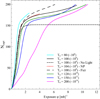 |
Fig. 1. Number of neutrons captured per heavy seed as a function of exposure ϕ for different temperatures (expressed in units of T6 = 106 K). The curves move from left to right with increasing temperature. The value in parentheses represents the typical neutron densities in cm−3 associated to the burning temperature. The T6 = 100, No Light case has the same composition as T6 = 100, but the abundance of nuclei with 13 < Ai < 56 is set to zero. The NP case accounts for enhanced abundances of neutron poisons (see text). The T6 = 100 – Fict case uses the fictitious network. |
where  is the thermal velocity of neutrons at temperature T and mn the neutron mass.
In the large network, the value of Ncapt changes through three types of reactions: a) neutron captures on heavy nuclei, b) production of nuclei with mass number A = 56 from neutron captures on lighter nuclei, and c) ejection of α particles during the Pb recycling chain of reactions. The first two reactions increase Ncapt, while the third reaction decreases it.
The evolution of Ncapt is primarily driven by neutron captures on 56Fe and its s-process progeny due to its dominant abundance. As is observed in Fig. 1, for higher neutron densities, greater neutron exposures are needed to attain the same value of Ncapt. This is explained by the fact that for increasing nn, the path of the s-process is shifted away from the valley of β− stability, toward more neutron-rich isotopes that have generally smaller neutron-capture cross sections. Therefore, a greater neutron exposure is needed to capture the same number of neutrons.
The effect of light species on Ncapt can be assessed by comparing the solid and dashed curves for T6 = 100. In the simulation without light species (elements with 13 < A < 56), Ncapt approaches the maximum value of Ncapt = 152, corresponding to the conversion of all the initial heavy seeds into 208Pb. Thereafter, the Pb recycling reactions are in equilibrium and freeze the abundances. On the other hand, when light species are included (solid black line), the limit on Ncapt is lifted as it can be further increased by the production of A = 56 nuclei from lighter species. These reactions affect Ncapt only in the very advanced stages of the s-process, when Ncapt ≳ 130.
To investigate the impact of a change in the species involved in the energy network (Z ≤ 17), we performed a simulation referred to as NP, in which the mass fraction of the light neutron poisons 14N, 16O, and 20Ne are multiplied by 10 with respect to their solar values and 22Ne, 23Na, and 25Mg are multiplied by 100, keeping all other nuclei with A > 13 at their solar abundance. With higher abundances of neutron absorbers, nn decreases, so that a slightly higher temperature is required to reach the same neutron density as in the T6 = 100 simulation. In this way, the differences between the two simulations result solely from the variation of the initial composition. As shown in Fig. 1, the effect of introducing the light neutron poisons is negligible. The NP simulation (dotted red line) closely follows the T6 = 100 simulation (solid black line). The NP simulation ends earlier (Ncapt = 178), however, because a larger fraction of the neutrons is captured before 13C is exhausted. We performed additional tests in which we varied the temperature, and we found in all cases that the addition of light neutron poisons has a very small effect: For the same neutron density, we have the same run of Ncapt as a function of exposure. In other words, for a given (nn, Ncapt), the reaction rates are almost not affected by the enhanced abundance of neutron poisons.
The comparison between the large (solid black line) and fictitious (dotted black line) networks in Fig. 1 at T6 = 100 shows good agreement, except at high exposures (ϕ ≳ 1.5 mb−1 or Ncapt ≳ 150), where Ncapt is overestimated in the fictitious network. The reason for this slight discrepancy is due to the emission of α-particles in the Pb-recycling reactions in the large network, which limits the increase in the mass fraction of the heaviest species. In this high Ncapt region, the fictitious network will overestimate Ncapt and potentially affect the interpolation of ⟨σv⟩(Ncapt, nn). Our simulations (Sect. 4) show, however, that this has a negligible impact on the final abundances of the fictitious particles.
Our choice of tabulating the reaction rates as functions of (Ncapt, nn) contrasts with the seminal work of Jorissen & Arnould (1989), where the authors considered only one fictitious particle (called heavy particle) to account for the neutrons captured by all particles with Ai ≥ 56 and tabulated the effective neutron-capture reaction rate as a function of exposure, yielding
where Yheavy(0) = ∑Ai ≥ 56Yi(0). As in our case, the function ⟨σv⟩heavy(ϕ) was extracted from one-zone nucleosynthesis calculations.
We illustrate in Fig. 2 our choice of interpolating variables on ⟨σv⟩heavy, but the conclusion that Ncapt is better suited than the exposition holds for all other effective reaction rates. Figure 2 shows ⟨σv⟩heavy as a function of Ncapt and ϕ. The burning temperature of 13C determines the neutron density during the nucleosynthesis and is indicated in parentheses.
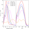 |
Fig. 2. ⟨σv⟩heavy (in units of [cm3 s−1 mol−1]) as a function of exposure ϕ (left panel) and number of neutrons captured per initial heavy seed Ncapt (right panel) for one-zone simulations where 13C burns at the temperatures indicated on the legend. The corresponding approximate neutron densities in cm−3 are indicated in parentheses. |
At the start (ϕ = 0 and Ncapt = 0), ⟨σv⟩heavy is mainly determined by the initial 56Fe, as it is the dominant nucleus. For increasing neutron densities, the s-process path encounters more n-rich nuclei that have smaller cross sections. Since ⟨σv⟩heavy is a weighted function of the individual capture rates, it is reduced when nn is larger (right panel of Fig. 2). For Ncapt ≳ 150, ⟨σv⟩heavy enters an asymptotic regime where all the heavy nuclei have been transformed into Pb and where light species (A ≤ 55) start being depleted. This slightly affects the capture rate.
We also note that with increasing neutron density, ⟨σv⟩heavy(ϕ) is shifted toward greater neutron exposures. This is a consequence of the global decrease in the effective capture rate with increasing nn. As neutrons are less efficiently captured, a higher exposure is required to reach the same value of Ncapt (Fig. 1).
When the variable Ncapt is used (right panel of Fig. 2), the shift is no longer present and the curves present an homothetic behavior. Consequently, if the neutron density changes, it is much easier to interpolate the rate as we can keep the same value of Ncapt. If the capture rates were tabulated as a function of ϕ, we would also need to adjust the exposure to account for the change in the neutron density. From now on, we only use Ncapt to describe the evolution of the reaction rates.
3.2. Effective reaction rates
The goal of this subsection is to explain the dependences of the reaction rates on Ncapt and nn. The behavior of ⟨σv⟩evo, k and ⟨σv⟩ncap, k is explained in terms of the distribution of nuclei to which they are connected via Eqs. (7) and (11). To discuss the dependence on Ncapt, we performed a one-zone nucleosynthesis simulation at T6 = 80 using a large network. This temperature was chosen so that the burning of 13C yields neutron densities lower than 2.5 × 106 cm−3 and the s-process follows the valley of stability closely. The resulting abundances and effective reaction rates of the fictitious particles are presented in Fig. 3.
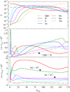 |
Fig. 3. Evolution of the abundances of fictitious particles Yk and the effective reaction rates ⟨σv⟩ncap and ⟨σv⟩evo (in units of [cm3 s−1 mol−1]) in terms of Ncapt for all fictitious particles. The computations are performed at T6 = 80, corresponding to a typical neutron density of 2.5 × 106 cm−3. |
We start the discussion on ⟨σv⟩evo, k by recalling that this reaction rate is driven mainly by the abundances of the border nuclei in Ek (Eq. (7)). If at a given time the distribution inside the fictitious particle is dominated by its lightest species, the evolution reaction rate will be low. Conversely, if the proportion of “border” nuclei increases with neutron captures, ⟨σv⟩evo, k will increase. We illustrate the discussion using lse as an example, for which we show in Fig. 4 several nuclear compositions for 88 ≤ A ≤ 137 taken at different values of Ncapt from our one-zone simulations. All the conclusions made for this particle can be extended to the other fictitious particles.
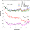 |
Fig. 4. Isotopic distributions of species included in lse (56 ≤ A ≤ 85) as a function of Ncapt. For the Ncapt = 126 and 160, the distributions have been renormalized to the abundance of the A = 91, Ncapt = 40 snapshot. They have been multiplied by a factor 7.3 and 27, respectively. |
We identify three successive regimes that govern ⟨σv⟩evo, k: the initial, intermediate, and asymptotic regimes. The initial regime affects particles with k ≥ ls, during which the behavior of the reaction rates depends heavily on the initial nuclear distribution. During the intermediate regime, the abundances and reaction rates are primarily driven by neutron captures on fe. Finally, during the asymptotic regime, the effects of neutron captures on nuclei lighter than 56Fe become apparent.
The initial regime is characterized by a decrease in ⟨σv⟩evo, k from its starting value until it reaches a global minimum. The middle panel of Fig. 3 shows that the minimum appears at higher Ncapt for heavier fictitious particles (ls = 5.6, lse = 13, hs = 22, and hse = 30). The lse and hse particles additionally show an initial spike at Ncapt = 0.8 and 1.75. To understand the behavior of ⟨σv⟩evo, we focused on the distribution of lse, whose evolution is presented in Fig. 4. Between Ncapt = 0 and 0.8, the number of lse border nuclei (with A = 136) increases by a factor ≈4 and yields the early rise in ⟨σv⟩evo, lse. After this initial adjustment, the lightest nuclei of lse start to be populated as a result of neutron captures on the abundant fe seeds. The relative abundance of lse border nuclei decreases until Ncapt = 11 and ⟨σv⟩evo, lse attains its minimum. At the end of the initial regime, the abundances of the various fictitious particles has increased by ≲500. The shape of the distribution, and by extension the magnitude of ⟨σv⟩evo, k during this phase, strongly depends on the initial composition.
The intermediate regime describes the region of moderate values of Ncapt where ⟨σv⟩evo, k increases steadily. It starts when ⟨σv⟩evo is minimum and ends when it reaches a maximum (Fig. 3). Again, heavier fictitious particles reach the end of the intermediate regime at higher Ncapt, ranging between 56 for fe and 160 for hse. The increase in ⟨σv⟩evo, k occurs in two phases, and we explain this behavior again using lse as a proxy. First, as shown in Fig. 4, between Ncapt = 11 and 40, neutron irradiation produces a rearrangement of the initial distribution, which flattens. The abundance of the border nuclei significantly increases and ⟨σv⟩evo, k rises. Then, around Ncapt = 40, neutron captures on 56Fe can no longer supply fresh nuclei to the fictitious particles. At this turning point, the abundance of the lightest elements (with A = 91) is maximum, and it subsequently decreases for higher Ncapt, while nuclei with A = 136 continue to be produced. At Ncapt = 126, ⟨σv⟩evo, lse reaches its peak value. During this intermediate phase, the shape of the elemental distribution is primarily determined by neutron captures on the abundant 56Fe and is almost independent of the initial mass fractions of the other nuclei.
The asymptotic regime starts after ⟨σv⟩evo has passed its maximum. The reaction rates undergo an initial decline due to the consumption of the border nuclei. They then remain roughly constant as abundances reach an equilibrium (Fig. 3).
We now analyze the behavior of ⟨σv⟩ncap, k (bottom panel of Fig. 3). In the initial regime, the behaviour of the internal neutron-capture rates depends on the initial composition, similarly to ⟨σv⟩evo, k. We see large variations (in particular in ⟨σv⟩ncap, hse) until the distribution of nuclei has readjusted. However, for such low Ncapt, the overabundance of fe with respect to the other fictitious particles implies that the latter have a negligible effects on the neutron density. In the intermediate and asymptotic regimes, the internal reaction rates remain roughly constant and weakly depend on Ncapt. This indicates a composition that is close to the nuclear equilibrium and that is illustrated for lse distributions at Ncapt = 40, 126, and 160.
The dependence of the reaction rates on the neutron density was assessed by performing one-zone simulations at temperatures varying between 80 ≤ T6 ≤ 200, thus probing neutron densities in the range 106 cm−3 − 1014 cm−3. The resulting ⟨σv⟩evo and ⟨σv⟩ncap are presented in Figs. 5 and 6, respectively. All reaction rates generally decrease with increasing nn. The reason is that the s-process path includes more nuclei with smaller cross sections.
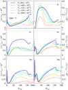 |
Fig. 5. Evolution of ⟨σv⟩evo, k (in units of [cm3 s−1 mol−1]) as a function of Ncapt for all fictitious particles and for different temperatures, as indicated on the graph. The corresponding neutron densities are given in parentheses. The reaction rate ⟨σv⟩evo, light has been multiplied by 5 for readability. |
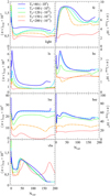 |
Fig. 6. Evolution of ⟨σv⟩ncap, k (in units of [cm3 s−1 mol−1]) as a function of Ncapt for all fictitious particles and for different temperatures, as indicated on the graph. The corresponding neutron densities are given in parentheses. |
A major branching point of the radiative s-process is at 85Kr. It activates at nn ≈ 108 cm−3 and greatly affects ⟨σv⟩evo, ls, as can be seen by comparing the T6 = 80 and 100 simulations in the middle left panel of Fig. 5. For nn ≥ 108 cm−3, the s-process path is diverted from 85Kr→ 85Rb→ 86Sr towards 85Kr→ 86Kr→ 87Rb. The last two nuclei are on the magic N = 50 isotone. They have small cross sections and cause a bottleneck for neutron captures. Their increased abundance causes the decrease in the evolution rate of ls following Eq. (7). For nn ≤ 1010 cm−3, the evolution reaction rates of the other fictitious particles conveniently show a weak dependence on nn.
For T6 = 80 and 100, ⟨σv⟩ncap varies only slightly with nn for all fictitious particles, with the exception of ls (Fig. 6). This is because they are associated with modest neutron densities (106 cm−3 < nn < 108 cm−3), so the path of the s-process essentially follows the valley of β− stability. The internal capture rate of ls is highest for T6 = 80 due to the absence of branching at 85Kr, as explained previously. For higher neutron densities, the presence of n-rich nuclei is more noticeable, especially for fe, lse, and hse particles, as seen by the much lower rates for T6 = 150 and 200. The internal reaction rates for fe, lse, and hse are most relevant for the accurate determination of nn because their cross section is highest (Eq. (12)). Particles lse and hse present an exceptionally flat behavior for Ncapt ≳ 30 because a nuclear equilibrium is reached in this regime.
4. Results using STAREVOL
Using the STAREVOL evolution code, we calculated the evolution of a 2 M⊙ star with [Fe/H] = −2 using the large network up to the end of the first 3DU to test the fictitious network during the radiative s-process. The convective-overshooting model described in Goriely & Siess (2018) was used to allow protons to spread past the convective envelope with an exponentially decreasing diffusion coefficient. This creates the 13C pocket necessary for the subsequent radiative s-process. For this case, we used diffusion parameters fover = 0.1, pover = 0.5, and Dmin = 106. Starting from this model, the interpulse nucleosynthesis was simulated using both the large and fictitious networks. The model was adapted to the fictitious network by converting mass fractions using Eq. (3).
We first analyze the shell at mass coordinate Mr = 0.599 M⊙, where the neutron density is maximum, reaching 5.17 × 107 cm−3. The corresponding evolution of neutron density, abundances, and effective reaction rates in both networks as functions of Ncapt are presented in Fig. 7. As discussed in Sect. 3.1, the Pb recycling reactions were not accounted for in the fictitious network, resulting in a noticeable increase in Ncapt in the region Ncapt ≳ 160. This effect can be observed in the uppermost panel of Fig. 7, where the final Ncapt reaches 205 in the large network and 210 in the fictitious network. The uppermost panel also agrees remarkably well for the neutron density profile in both networks; the differences do not exceed 3% (when the comparison is done at a given time t, as opposed to a comparison at a similar Ncapt). The abundances of fictitious particles in both networks also agree well. Slight differences that do not exceed 0.3 dex are observed and mainly affect ls.
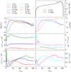 |
Fig. 7. Evolution of the neutron density (first row), abundances of fictitious particles (second row), effective neutron-capture reaction rates ⟨σv⟩ncap, k (third row) and reaction rates ⟨σv⟩evo, k (fourth row) as a function of Ncapt during the first interpulse phase in a star of 2 M⊙ and [Fe/H] = −2 at the mass coordinate Mr = 0.599 M⊙. The reaction rates are given units of [cm3 s−1 mol−1]. |
The third row of Fig. 7 shows the values of ⟨σv⟩ncap, k as a function of Ncapt. The effective neutron-capture rates are well reproduced for all fictitious particles. The largest differences are observed for hse and for ls in the region Ncapt ≥ 150, but they never exceed 5%.
The evolution reaction rates (final row of Fig. 7) are also well reproduced. The largest differences arise during the intermediate phase, in which the fictitious reaction rates are slightly underestimated. They have a limited impact on the abundances of the fictitious particles, however.
The reaction rate ⟨σv⟩evo, ls shows the greatest deviations and can be underestimated by as much as ≈20%. This is explained by the differences in the evolution of nn during the nucleosynthesis shown here and the one used to tabulate ⟨σv⟩evo, ls and the activation of the branching point at 85Kr occurring at nn = 108 cm−3. During the radiative s-process, the temperature rises gradually, and the neutron density increases over time as the 13C(α, n) reaction is more efficiently activated. The neutron densities initially favor the decay of 85Kr, and 85Rb is produced at the expense of 86Kr, which is more difficult to destroy due to its low cross section. In the one-zone simulations, the neutron density is approximately constant, and a larger amount of 86Kr is produced. As 86Kr is not a border nucleus of ls, its higher abundance in one-zone simulations than during the radiative s-process is responsible for the lower value of ⟨σv⟩evo, ls in the fictitious network.
The evolution of the abundances of the fictitious particles  averaged over the radiative shells where Ncapt > 3 is presented in Fig. 8. In these layers, the s-process has taken place, and the resulting nucleosynthesis is ingested in the thermal pulse. By performing the average, we assessed which elements are effectively produced during the interpulse and are brought to the surface of the star. In this low-mass star model, the nucleosynthesis occurring in the thermal pulse is unlikely to change the distribution of the fictitious particles, but this may be different in higher-mass stars (see Appendix A). The averaged abundance contains the nucleosynthesis products of layers exposed to a wide range of neutron densities.
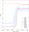 |
Fig. 8. Averaged abundances of fictitious particles |

At the start of the radiative s-process, the fictitious particles ls, lse, hs and hse are successively produced (Fig. 8). The slight decrease that follows the maximum of  results from the layers where the neutron density was the highest and the s-process was sufficiently advanced to start the destruction of the fictitious particles. This destruction was counterbalanced by the production of fictitious particles in neighboring layers, however, where the neutron density was lower. In this simulation, fe is only consumed and vhs is produced. There is a very good agreement in
  for all fictitious particles at all times. The largest differences are for ls and lse and do not exceed < 0.1 dex.
Pulse after pulse, the composition of the layers below the convective envelope is progressively enriched in heavy species and can show substantial differences with respect to the solar-scaled composition that was used to compute ⟨σv⟩evo, k and ⟨σv⟩ncap,k. To test how robust our estimation of the fictitious reaction rates is, we performed new calculations with the fictitious and the large networks using the conditions at the beginning of the seventh interpulse of our 2 M⊙, [Fe/H]= − 2 stellar model. At this time, the abundance of the heavy nuclei is increased by a factor of ≈50 compared to the initial solar value, but for some s-process elements, this enhancement can reach almost 3 dex, such as for 208Pb. On the other hand, the abundance of 56Fe is almost not affected because it was replenished by the previous 3DU episode. In this test simulation, the composition of the fictitious abundances was adjusted to this new structure using Eq. (3), but the fictitious reaction rates were kept unchanged and were tabulated using the initial solar-scaled composition.
Figure 9 shows the evolution of the abundances and reaction rates of the fictitious particles in the most irradiated shell as a function of Ncapt, which is a proxy for time. The enrichment in heavy species can be assessed by comparing the upper panel of Fig. 9 with the middle panel of Fig. 7. Small differences are observed for hs and hse at the beginning of the interpulse, but they disappear as soon as Ncapt ≳ 30, that is, when nucleosynthesis enters the intermediate regime. For the other elements, the agreement is excellent.
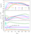 |
Fig. 9. Evolution of the abundances and reaction rates in the units of [cm3 s−1 mol−1]: as a function of Ncapt in the large (full lines) and fictitious (dashed lines) networks during the seventh interpulse of a 2 M⊙, [Fe/H] = −2 star. The effective neutron-capture rate of ls, hs, and vhs was multiplied by 10 for readability. |
Relatively large variations are present initially for particles more massive than fe concerning ⟨σv⟩evo (middle panel of Fig. 9), but again, they are significantly reduced when the intermediate regime is reached (after ⟨σv⟩evo has passed its global minimum). For higher Ncapt, the differences are comparable to those presented in Fig. 7. The same conclusions hold for ⟨σv⟩ncap shown in the bottom panel: The reaction rates are somewhat discrepant for low Ncapt, but become very comparable in the intermediate regime. We also computed the averaged abundance of the fictitious particles over the shells that have reached Ncapt > 3 at the end of the interpulse. The resulting abundances between the large and fictitious network do not differ by more than 0.1 dex for the early pulse case. In conclusion, our tests show that the fictitious network is weakly dependent on the composition in heavy elements of the intershell as long as the nucleosynthesis enters the intermediate regime, which is characterized by Ncapt ≥ 30 and corresponds to a neutron exposure ϕ ≳ 0.5 mb−1 (Fig. 1). For completion, we present in the appendix the performance of the fictitious network under convective s-process nucleosynthesis and highlight some limitations of this model.
5. Discussion
We have presented a fictitious network that contains an inert neutron and seven fictitious particles, each representing the abundances of groups of nuclei involved in the s-process nucleosynthesis. Their effective reaction rates were tabulated as functions of Ncapt and nn using one-zone nucleosynthesis simulations. In contrast to Jorissen & Arnould (1989), we used Ncapt instead of the exposure ϕ. This resulted in an easier and more consistent interpolation of the rates when the neutron density varied strongly.
The network was tested on a 2 M⊙, [Fe/H] = −2 star for the radiative s-process. We found that the production of fictitious particles and the neutron density are correctly reproduced. For a typical radiative s-process that reaches Ncapt ≳ 30 (ϕ ≳ 0.5 mb−1), we found that the reaction rates enter the so-called intermediate regime in which the final abundances are primarily determined by the initial 56Fe abundance and weakly depend on the initial distribution of heavy nuclei.
In Appendix A, the convective s-process is tested on the 19th pulse of a 3 M⊙, [Fe/H] = −2.5 star. In this case, the fictitious network performance is lower. While the final abundances of the fe, ls, hse, and vhs are fairly well reproduced, the abundances of lse and hs showed some disagreements. This is ascribed to two factors. First, the composition irradiated during the thermal pulse can differ significantly from the initial composition as a result of past s-process episodes, and the tabulated reaction rates are no longer correct. Second, the convective s-process does not lead to sufficient neutron captures, so that the intermediate regime cannot be reached, where abundances are mainly determined by the initial 56Fe. We tried to approximate the correct reaction rates based on the composition of the material entering the thermal pulse. This led to a significant improvement for the lse particle, but hs remained poorly determined. To conclude, our fictitious network is able to trace the production of s-process elements in radiative layers fairly well, but shows limitations when dealing with the convective s-process. It is suited for low-mass AGB stars and represents a substantial improvement compared to the previous formalism developed by Jorissen & Arnould (1989).
Acknowledgments
L.S. is senior FRS-F.N.R.S. research associate.
References
- Arlandini, C., Kappeler, F., Wisshak, K., et al. 1999, ApJ, 525, 886 [NASA ADS] [CrossRef] [Google Scholar]
- Asplund, M., Grevesse, N., Sauval, A. J., & Scott, P. 2009, ARA&A, 47, 481 [NASA ADS] [CrossRef] [Google Scholar]
- Battino, U., Tattersall, A., Lederer-Woods, C., et al. 2019, MNRAS, 489, 1082 [Google Scholar]
- Bisterzo, S., Gallino, R., Käppeler, F., et al. 2015, MNRAS, 449, 506 [Google Scholar]
- Campbell, S. W., & Lattanzio, J. C. 2008, A&A, 490, 769 [NASA ADS] [CrossRef] [EDP Sciences] [Google Scholar]
- Choplin, A., Siess, L., & Goriely, S. 2021, A&A, 648, A119 [NASA ADS] [CrossRef] [EDP Sciences] [Google Scholar]
- Cristallo, S., Piersanti, L., Straniero, O., et al. 2011, ApJS, 197, 17 [NASA ADS] [CrossRef] [Google Scholar]
- Cruz, M. A., Serenelli, A., & Weiss, A. 2013, A&A, 559, A4 [NASA ADS] [CrossRef] [EDP Sciences] [Google Scholar]
- Denissenkov, P. A., & Tout, C. A. 2003, MNRAS, 340, 722 [NASA ADS] [CrossRef] [Google Scholar]
- Forestini, M., Goriely, S., Jorissen, A., & Arnould, M. 1992, A&A, 261, 157 [NASA ADS] [Google Scholar]
- Gil-Pons, P., Doherty, C. L., Gutiérrez, J., et al. 2021, A&A, 645, A10 [EDP Sciences] [Google Scholar]
- Goriely, S., & Mowlavi, N. 2000, A&A, 362, 599 [NASA ADS] [Google Scholar]
- Goriely, S., & Siess, L. 2005, in From Lithium to Uranium: Elemental Tracers of Early Cosmic Evolution, eds. V. Hill, P. Francois, & F. Primas, 228, 451 [Google Scholar]
- Goriely, S., & Siess, L. 2018, A&A, 609, A29 [NASA ADS] [CrossRef] [EDP Sciences] [Google Scholar]
- Herwig, F. 2005, ARA&A, 43, 435 [NASA ADS] [CrossRef] [Google Scholar]
- Herwig, F., Langer, N., & Lugaro, M. 2003, ApJ, 593, 1056 [NASA ADS] [CrossRef] [Google Scholar]
- Jorissen, A., & Arnould, M. 1989, A&A, 221, 161 [Google Scholar]
- Kappeler, F., Beer, H., & Wisshak, K. 1989, Rep. Prog. Phys., 52, 945 [Google Scholar]
- Karakas, A. I., & Lattanzio, J. C. 2003, PASA, 20, 279 [NASA ADS] [CrossRef] [Google Scholar]
- Karakas, A. I., & Lattanzio, J. C. 2014, PASA, 31 [CrossRef] [Google Scholar]
- Langer, N., Arcoragi, J. P., & Arnould, M. 1989, A&A, 210, 187 [NASA ADS] [Google Scholar]
- Lugaro, M., Karakas, A. I., Stancliffe, R. J., & Rijs, C. 2012, ApJ, 747, 2 [Google Scholar]
- Neyskens, P., van Eck, S., Jorissen, A., et al. 2015, Nature, 517, 174 [NASA ADS] [CrossRef] [Google Scholar]
- Nucci, M. C., & Busso, M. 2014, ApJ, 787, 141 [NASA ADS] [CrossRef] [Google Scholar]
- Siess, L., & Arnould, M. 2008, A&A, 489, 395 [NASA ADS] [CrossRef] [EDP Sciences] [Google Scholar]
- Straniero, O., Gallino, R., Busso, M., et al. 1995, ApJ, 440, L85 [NASA ADS] [CrossRef] [Google Scholar]
- Trippella, O., Busso, M., Palmerini, S., Maiorca, E., & Nucci, M. C. 2016, ApJ, 818, 125 [Google Scholar]
- Vescovi, D., Cristallo, S., Busso, M., & Liu, N. 2020, ApJ, 897, L25 [Google Scholar]
Appendix A: Convective s-process
In the large network, the calculation of the nucleosynthesis in convective zones is done in the one-zone approximation, in which the mass fraction of all elements, except neutrons, is averaged across the mixed region. The reaction rates are computed locally and are then mass averaged over the extent of the convective region,
where the subscript j refers to quantities evaluated at the shell j, and dmj is the mass of this shell. This expression applies to all reactions except neutron captures because the short lifetime of neutrons means that their local abundance must be used. For the averaged neutron-capture rate, the following expression is used:
We applied the fictitious network on the 19th thermal pulse of a 3 M⊙, [Fe/H]=-2.5 star. The pulse-driven convective zone covers the mass coordinates between mbot = 0.810002 M⊙ and mtop = 0.817528 M⊙ at its maximum extent. The temperature at the base of the convective zone reached T = 3.8 × 10⁸K, activating the 22Ne(α, n) 25Mg reaction and resulting in a peak neutron density of 8.2 × 1013 cm−3. The thermal pulse lasted for 39 years. In these conditions, ten neutrons are captured by heavy nuclei in the convective shell by the end of the thermal pulse on average.
Starting from the same model computed with the large network just before the thermal pulse, we followed the nucleosynthesis using our formalism, setting the initial composition of the fictitious model using Eq. (3). We followed the abundances  of fictitious particles averaged over the maximum extent of the convective zone (i.e., between mbot and mtop) throughout the duration of the pulse. The results are presented in Fig. A.1. The convective zone is present between models 60609 and 61002. The figure shows that the changes in
  occur between models 60640 and 60680, where the neutron density exceeds ≈1012 cm−3. Outside these models, nn is too low and the neutron-capture nucleosynthesis is inefficient.
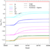 |
Fig. A.1. Evolution of the averaged abundances of the fictitious particles during the convective s-process in a 3M⊙, [Fe/H]=-2.5 star using the large network (Large; solid line), the fictitious network without modifications (Fictitious; dashed line), and the fictitious network with approximated reaction rates (Fictitious + Approx; dotted line). The abundances are averaged over the maximum extent of the convective shell (0.810 ≤ Mr/M⊙ ≤ 0.817528). The mean abundance Yvhs is multiplied by 10−0.2 to distinguish it from Yhse. The thermal pulse starts at model 60609 and ends at model 61002, corresponding to a duration of 39 years. |
In the large network, the abundances of ls, lse, hs, and hse have increased by 0.6 − 0.7 dex and by 0.3 dex for vhs. The abundance of fe has dropped by only 0.02 dex. The lse and hs particles are underproduced by the fictitious network by 0.4 and 0.3 dex, respectively. The agreement for ls and vhs is better, as the final abundances are within 0.1 dex of the large network. Only hse is close to the large network value. The discrepancies between the two networks for the convective s-process are more pronounced than in the radiative case.
Two main factors can explain the weaker performance of the fictitious network. The low efficiency of the convective s-process prevents the nucleosynthesis from entering the intermediate regime, where the abundances are mostly determined by neutron captures on 56Fe and weakly depend on the distribution of the other elements. The convective s-process thus depends on the composition of heavy elements at the start of the neutron irradiation episode, which in the convective shell can differ strongly from the initial distribution used to tabulate the reaction rates due to 3DU episodes, for example.
We present in Fig. A.2 the composition of the matter entering the thermal pulse (Ypulse). It is made of layers, located below m3DU, the mass coordinate corresponding to the maximum extent of the convective envelope during the previous 3DU, which belonged to the previous pulse. It carries the products of the last convective s-process, and its composition Y1 shows depletion in 56Fe and enrichment in light s-elements. The mass of this layer is Δm1 = m3DU − mbot, and Y1 is characterized by Ncapt = 10.15, meaning that it mostly contains light s-elements. The layers between m3DU and mtop contain the envelope composition after the dredge-up and has been processed by H-burning during the interpulse period. Its composition Y2 has 56Fe close to the initial value and is slightly enriched in heavier s-elements from the previous 3DU episodes. The mass of this layer is Δm2 = mtop − m3DU, and its composition is characterized by Ncapt = 1. In our model, we have Mpulse = Δm1 + Δm2 and Ypulse = (Y1Δm1 + Y2Δm2)/Mpulse. In Fig. A.2, Y1 is scaled up to match the value of Ypulse at A = 136 to show that it is almost identical to Yconv for most nuclei. In fact, Y1 provides 92% of nuclei with 60 ≤ A ≤ 142 and 82% of nuclei with A ≥ 143. The distribution near the iron peak is determined by Y2, which is very rich in these elements.
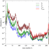 |
Fig. A.2. Distribution of elements entering the pulse composition. Ypulse is the average composition in the thermal pulse, Y1 and Y2 are the average compositions between mbot and m3DU and m3DU and mtop, respectively. Both are computed a few models before the thermal pulse. Yini is the initial distribution of nuclei in the star. |
The mixing of Y1 and Y2 has two important consequences. First, the value of Ncapt in the pulse drops to ∼3.17; the exact value depends on Δm1 and on the efficiency of the previous convective s-process. In this regime of low Ncapt, the reaction rates for fe are fairly insensitive to nn (Figs. 5 and 6), even though neutron densities can vary sharply over several orders of magnitude in the pulse. Second, ⟨σv⟩ncap, fe (Eq. 11) depends on the most abundant element in fe, that is, 56Fe. Since the abundance of fe is weakly affected in the pulse, ⟨σv⟩ncap, fe will not be strongly impacted by the change in the distribution of the heavy nuclei.
Concerning ⟨σv⟩evo, fe, the numerator of Eq. (7) is proportional to the abundances of nuclei with A = 85 and the denominator is mainly determined by the abundance of 56Fe. The abundance of A = 85 nuclei in the pulse cannot be known beforehand, but it will always be greater than its initial value, since the products of the last s-process are mixed in the convective shell. It is thus expected that the tabulated ⟨σv⟩evo, fe will be underevaluated and the fe particle will not be consumed as efficiently in the fictitious network as it is in the large one.
Concerning the reaction rates of the heavier fictitious particles (for nuclei with A ≥ 86), given the similarity between the pulse (Ypulse) and irradiated (Y1) distributions, we expect that the effective reaction rates that were calculated in the radiative case will remain applicable. With this insight, we modified the calculation of the fictitious rate to improve our treatment of the convective s-process. In practice, for k > fe, the reaction rate for the fictitious particle k in the convection zone was calculated taking the average rate over the pulse overlap region 1 only,
and for the rates involving fe, we kept the standard procedure. The results of the corrected fictitious network (Fictitious + Approx) are also displayed in Fig. A.1. The agreement for lse and vhs particles is considerably improved and remains the same for ls and hse. Unfortunately, hs is now overproduced, but the difference with the large network is on the same order as before.
To summarize, the dilution of irradiated material in the pulse modifies the distribution of chemical elements that is expected from a pure radiative s-process. This alteration does not impact the rate of ⟨σv⟩ncap, fe because this rate mainly depends on the fe abundance, which is weakly affected. For the heavier fictitious particles, the agreement is acceptable and improved if the reaction rates are averaged over the region that is rich in heavy nuclei between mbot and m3DU.
All Tables
Fictitious particles are constructed by grouping nuclei with atomic mass number Ak, min ≤ Ai ≤ Ak, max.
All Figures
|
Fig. 1. Number of neutrons captured per heavy seed as a function of exposure ϕ for different temperatures (expressed in units of T6 = 106 K). The curves move from left to right with increasing temperature. The value in parentheses represents the typical neutron densities in cm−3 associated to the burning temperature. The T6 = 100, No Light case has the same composition as T6 = 100, but the abundance of nuclei with 13 < Ai < 56 is set to zero. The NP case accounts for enhanced abundances of neutron poisons (see text). The T6 = 100 – Fict case uses the fictitious network. |
| In the text | |
|
Fig. 2. ⟨σv⟩heavy (in units of [cm3 s−1 mol−1]) as a function of exposure ϕ (left panel) and number of neutrons captured per initial heavy seed Ncapt (right panel) for one-zone simulations where 13C burns at the temperatures indicated on the legend. The corresponding approximate neutron densities in cm−3 are indicated in parentheses. |
| In the text | |
|
Fig. 3. Evolution of the abundances of fictitious particles Yk and the effective reaction rates ⟨σv⟩ncap and ⟨σv⟩evo (in units of [cm3 s−1 mol−1]) in terms of Ncapt for all fictitious particles. The computations are performed at T6 = 80, corresponding to a typical neutron density of 2.5 × 106 cm−3. |
| In the text | |
|
Fig. 4. Isotopic distributions of species included in lse (56 ≤ A ≤ 85) as a function of Ncapt. For the Ncapt = 126 and 160, the distributions have been renormalized to the abundance of the A = 91, Ncapt = 40 snapshot. They have been multiplied by a factor 7.3 and 27, respectively. |
| In the text | |
|
Fig. 5. Evolution of ⟨σv⟩evo, k (in units of [cm3 s−1 mol−1]) as a function of Ncapt for all fictitious particles and for different temperatures, as indicated on the graph. The corresponding neutron densities are given in parentheses. The reaction rate ⟨σv⟩evo, light has been multiplied by 5 for readability. |
| In the text | |
|
Fig. 6. Evolution of ⟨σv⟩ncap, k (in units of [cm3 s−1 mol−1]) as a function of Ncapt for all fictitious particles and for different temperatures, as indicated on the graph. The corresponding neutron densities are given in parentheses. |
| In the text | |
|
Fig. 7. Evolution of the neutron density (first row), abundances of fictitious particles (second row), effective neutron-capture reaction rates ⟨σv⟩ncap, k (third row) and reaction rates ⟨σv⟩evo, k (fourth row) as a function of Ncapt during the first interpulse phase in a star of 2 M⊙ and [Fe/H] = −2 at the mass coordinate Mr = 0.599 M⊙. The reaction rates are given units of [cm3 s−1 mol−1]. |
| In the text | |
|
Fig. 8. Averaged abundances of fictitious particles |
| In the text | |
|
Fig. 9. Evolution of the abundances and reaction rates in the units of [cm3 s−1 mol−1]: as a function of Ncapt in the large (full lines) and fictitious (dashed lines) networks during the seventh interpulse of a 2 M⊙, [Fe/H] = −2 star. The effective neutron-capture rate of ls, hs, and vhs was multiplied by 10 for readability. |
| In the text | |
|
Fig. A.1. Evolution of the averaged abundances of the fictitious particles during the convective s-process in a 3M⊙, [Fe/H]=-2.5 star using the large network (Large; solid line), the fictitious network without modifications (Fictitious; dashed line), and the fictitious network with approximated reaction rates (Fictitious + Approx; dotted line). The abundances are averaged over the maximum extent of the convective shell (0.810 ≤ Mr/M⊙ ≤ 0.817528). The mean abundance Yvhs is multiplied by 10−0.2 to distinguish it from Yhse. The thermal pulse starts at model 60609 and ends at model 61002, corresponding to a duration of 39 years. |
| In the text | |
|
Fig. A.2. Distribution of elements entering the pulse composition. Ypulse is the average composition in the thermal pulse, Y1 and Y2 are the average compositions between mbot and m3DU and m3DU and mtop, respectively. Both are computed a few models before the thermal pulse. Yini is the initial distribution of nuclei in the star. |
| In the text | |
Current usage metrics show cumulative count of Article Views (full-text article views including HTML views, PDF and ePub downloads, according to the available data) and Abstracts Views on Vision4Press platform.
Data correspond to usage on the plateform after 2015. The current usage metrics is available 48-96 hours after online publication and is updated daily on week days.
Initial download of the metrics may take a while.