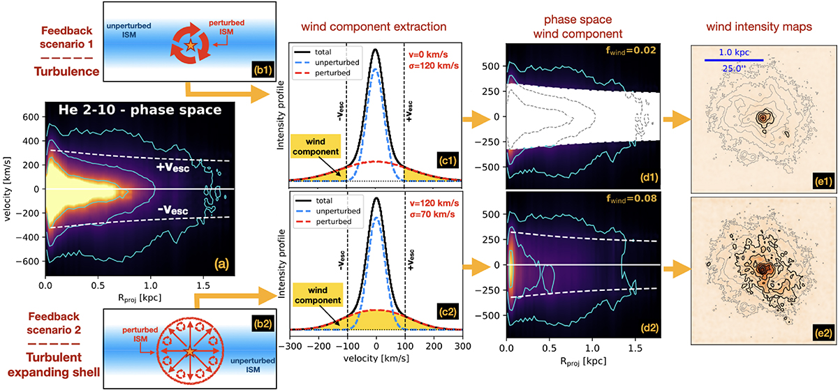
Scheme illustrating the extraction of the wind component from the Hα velocity cube of He 2-10. (a): phase-space distribution for the whole Hα emission. Instrumental broadening is removed via the multi-Gaussian decomposition. Cyan contours encompass 50%, 70%, and 90% of the total Hα flux. White-dashed lines show the escape speed radial profile (see Sect. 4.1). (b): the two feedback scenarios of Sect. 4.2. In (b1) feedback injects turbulence in the ISM, but produces no bulk flow. In (b2) feedback produces the spherical expansion of a turbulent shell of gas (TES). (c): illustration of the effects of feedback on a single velocity profile. For both scenarios we assume v_esc of 100 km s⁻¹, a systemic velocity of 0 km s⁻¹, and velocity dispersion of 30 km s⁻¹ for the unperturbed gas (blue-dashed curve). The component perturbed by feedback (red-dashed curve) is derived by assuming a shell expansion speed, v, and a velocity dispersion, σ, indicated in the top-right corner. Both scenarios feature very similar broad components. In the turbulent case (c1), only the flux at |v|> v_esc (highlighted in yellow) is eligible as ‘wind’. In the TES case, given that v > v_esc, the whole component will be associated with a wind. (d): phase-space plots for the wind component alone, extracted by processing each Hα velocity profile as discussed in Sect. 4.2. Contours are defined as in panel a. (e): integrated Hα intensity maps of the wind component. Iso-intensity contours for the total Hα emission are shown in grey, as a reference.