© G. B. Valsecchi et al. 2022

1 Introduction

Until 1999, among Solar System small bodies, only comets were known to possibly move in retrograde heliocentric orbits, with the implicit understanding that the reversal of their sense of motion had taken place, in most cases, due to the action of external perturbers at vast distances from the Sun, while residing in the Oort Cloud. The situation changed in June 1999, with the discovery of the first two retrograde asteroids, 1999 LD₃₁¹ and 1999 LE₃₁²; the former has since been numbered and named as (20461) Dioretsa, the name being the word ‘asteroid’ spelt backwards. The following years saw an increase in the number of known asteroids in retrograde orbits; as of 15 July 2022, there are 21 such asteroids among the numbered ones, and 58 among the multi-opposition ones, as reported in AstDyS³.

The possible processes that have transformed the orbits of these asteroids from direct to retrograde include:

• residence in the Oort cloud, followed by planetary capture, and in this case, the asteroid may be an extinct comet;

• chaotic evolution to mean-motion or degenerate secular resonance (such as the v₆), with large amplitude changes to inclination (Greenstreet et al. 2012), helped by the eccentric Lidov-Kozai mechanism (Lithwick & Naoz 2011; Naoz et al. 2017);

• close encounter with a planet.

This last mechanism was pointed out by Rickman et al. (2017), who numerically integrated the evolution of 100 000 fictitious comets, for a maximum of 100 000 orbital revolutions each, in a model Solar System consisting of the Sun and the four giant planets (for details, see Rickman et al. 2017).

Their initial population of comets came from the end state of the computations of Brož et al. (2013), who simulated the flux of comets in the inner part of the Solar System in the framework of the Nice model. From that end state, Rickman et al. (2017) extracted, at random, 5000 sets of a, q, i, characterized by orbital period P < 20 yr and the Tisserand parameter⁴ with respect to Jupiter T_J > 2; each set was cloned 20 times, assigning values of Ω, ω, M taken at random from flat distributions.

Among the many results by Rickman et al. (2017), those for the comets that had flipped from direct to retrograde orbits were the starting point for the analysis presented in this paper. It was found that:

• 12 comets were transferred to retrograde orbits and remained retrograde until the end of the integration;

• the final orbits of these 12 comets were characterized by P < 20 yr, T_J < 2;

• 417 comets performed at least one revolution with i > 90°; defining ‘retrograde visits’ as sequences of at least ten retrograde revolutions, the 417 comets made a total of 514 retrograde visits;

• 299 of these 417 ended up colliding with the Sun, of which 177 while still on retrograde orbits, and 122 on prograde orbits;

• at the end of the integration, 25 comets that had passed through a retrograde phase had returned to prograde motion.

A considerable fraction of the inclination flips were caused by close encounters with Jupiter; the exact amount could not be ascertained, since this phenomenon had not been taken into account when planning the integration output. In this paper we examine the issue, with the goal of understanding this dynamical path to retrograde motion in the light of the analytical theory of close encounters (Öpik 1976; Greenberg et al. 1988; Carusi et al. 1990; Valsecchi et al. 2003; Valsecchi 2006).

We proceed as follows. In Sect. 2, we discuss the role of close encounters with the giant planets in the dynamics of small bodies in the framework of the analytical theory, and derive the conditions on orbital parameters that enable the inclination flips. In Sect. 3, we check the validity of the theory by numerical integrations. In Sect. 4, some implications of our results are discussed, while in Sect. 5 we draw the conclusions. Appendices A and B deal with some technical issues that are treated separately in order not to disrupt the flow of the paper.

2 Close encounters

2.1 The Tisserand parameter

The orbits of comets and asteroids in the outer planetary region are strongly affected by close encounters with the giant planets that make the orbits of these small bodies chaotic. In fact, a close encounter can drastically change the orbital elements of a small body, as is well known since the pioneering papers by Lexell and LeVerrier (see Valsecchi 2007 and references therein).

In this respect, Tisserand (1889a,b) introduced a quantity, often called the Tisserand invariant or the Tisserand parameter, which is nearly conserved across a close encounter, even in cases in which the orbit of the small body is strongly altered. The Tisserand parameter can be derived from the Jacobi constant of the restricted, circular, three-dimensional three-body problem (hereafter RC3D3BP), neglecting the terms that are multiplied by the mass of the planet (Roy 2005), and its conservation expresses the conservation of the modulus of the planetocentric velocity of the small body.

Thus, in the RC3D3BP, the effect of a close encounter with a planet is a change in the direction of the planetocentric velocity vector. This property is exploited in the analytical theory of close encounters that is used in this paper.

Although the actual motion of a small body in the outer planetary region can be influenced by more complex perturbations than those present in the RC3D3BP, some general results that can be deduced from the latter are useful in order to understand some of the overall features of the dynamics in that region. In fact, the use of the RC3D3BP is justified by the smallness of the eccentricities of the Solar System planets, and by their hierarchical arrangement, with almost coplanar orbits separated by distances that are very large compared to the planetocentric distance at which a small body has to pass in order to be strongly perturbed.

The pioneer of the use of the Tisserand parameter to classify the motions of small bodies was Kresák (1972a); in particular, he set the dividing line between asteroids and Jupiter family comets (JFCs, historically defined as having orbital period P < 20 yr) at T_J = 3, where T_J is the Tisserand parameter computed with respect to Jupiter (Kresák 1972b). In the same spirit, Carusi et al. (1987) proposed that the dividing line between JFCs and Halley-type comets (HTCs, historically defined as having 20 < P < 200 yr) be set at T_J = 2. Thus, JFCs have 3 > T_J > 2, while HTCs have T_J < 2; it should be noted that many HTCs are on retrograde orbits. Moreover, not only HTCs, but also an increasing number of asteroids are found to be on retrograde orbits; among them, perhaps not surprisingly, are many Damocloids⁵, defined as having T_J < 2 (Jewitt 2005).

Computations by Levison & Duncan (1994) showed that transitions between JFCs and HTCs, defined according to Carusi et al. (1987), are rather rare; again in the same spirit, Levison (1996) proposed calling comets with T_J > 2 ‘ecliptic comets’, and those with T_J < 2 ‘isotropic comets’, due to the presence of all inclinations among the latter.

2.2 Conditions enabling inclination flips

As shown by Tisserand (1889a,b), in the RC3D3BP Sun-planet-small body the occurrence of a close encounter leaves nearly invariant the quantity:

$$T_{\text{p}}=\frac{a_{\text{p}}}{a}+2\sqrt{\frac{a\left(1-e^2\right)}{a_{\text{p}}}}\cos i,$$(1)

where T_p is the Tisserand parameter computed with respect to planet p, a_p is the radius of the circular orbit of the planet, and a, e and i are the semi-major axis, eccentricity and inclination of the orbit of the small body, computed with respect to the plane in which the planet moves.

As is well known, the constancy of T_p reflects the constancy of the difference between the orbital energy and the third component of the orbital angular momentum (Valsecchi et al. 1999):

$$T_{\text{p}}=2\left(L_{z,\text{p}}-E_{\text{p}}\right),$$(2)

where

$$L_{z,p}=\sqrt{\frac{a\left(1-{\text{e}}^2\right)}{a_{\text{p}}}}\cos i$$(3)

is the third component of the specific angular momentum and

$$E_{\text{p}}=-\frac{a_{\text{p}}}{2a}$$(4)

is the specific orbital energy, both in units of the corresponding quantities for planet p.

The sign of L_z,p determines the sense of motion, direct for L_z,p > 0 and retrograde for L_z,p < 0. The frontier between these two regimes of motion is L_z,p = 0, which corresponds either to i = 90°, in which case the motion is neither direct nor retrograde, or to the perihelion distance q = 0, that is, to a rectilinear orbit.

In order to possibly flip between direct and retrograde motions, the orbit of a small body must pass through the condition L_z,p = 0; in that case Eq. (2) becomes:

$$T_{\text{p}}=-2E_{\text{p}}=\frac{a_{\text{p}}}{a},$$(5)

with the important consequence that, for inclination flips to be at all possible as a consequence of an encounter with planet p, T_p must obey:

$$T_{\text{p}}<2,$$(6)

since for a < a_p/2 the orbits of the planet and of the small body cannot cross. Another consequence is that, for T_p < 2, the semi-major axis value:

$$a*=\frac{a_p}{T_p}.$$(7)

sets a dividing line: if a < a* the orbit is retrograde, and if a > a* the orbit is prograde.

We now put the equations that we have just obtained in the framework of the analytical theory of close encounters (Öpik 1976; Greenberg et al. 1988; Carusi et al. 1990; Valsecchi et al. 2003; Valsecchi 2006), in which it is convenient to substitute a, e, i of the small body with three other quantities, the modulus of planetocentric encounter velocity U_p = U_p(a, e, i), and the angles θ_p = θ_p(a, U_p), ϕ_p = ϕ_p(a, e, i, ω, f_b), that define its direction. For the moment we need only the explicit expressions for U_p and cos θ_p (by definition 0° ≤ θ_p ≤ 180°).

The modulus of the planetocentric velocity of the small body U_p is computed from T_p:

$$U_{\text{p}}=\sqrt{3-T_{\text{p}}}=\sqrt{3-\frac{a_{\text{p}}}{a}-2\sqrt{\frac{a\left(1-{\text{e}}^2\right)}{a_{\text{p}}}}\cos i}.$$(8)

From U_p and a we can compute θ_p, the angle in the range (0°, 180°) between the planetocentric encounter velocity vector U_p and the heliocentric velocity of the planet:

$$\cos {\theta }_{\text{p}}=\frac{1-U_{\text{p}}^2-\frac{a_{\text{p}}}{a}}{2U_{\text{p}}}$$(9)

$$\sin {\theta }_{\text{p}}=\sqrt{1-{\cos }^2{\theta }_{\text{p}}};$$(10)

in these expressions, U_p is in units of the heliocentric velocity of the planet encountered. It is important to notice that e and i enter the expressions for U_p and θ_p only through the product $\sqrt{1-{\text{e}}^2}\cos i$. Substituting a* from Eq. (7) in Eq. (9) it is easy to show that when L_z,p = 0, the corresponding value of θ*_p is given by:

$$\cos {\theta }_{\text{p}}^{*}=-\frac{1}{U_{\text{p}}}.$$(11)

The previous results can be summarized as follows:

• the transition to a retrograde orbit due to a close encounter can take place only if U_p ≥ 1, that is, T_p ≤ 2, no matter what the mass of the planet is;

• the dividing line at T_J = 2 between JFCs and HTCs introduced by Carusi et al. (1987) makes celestial mechanical sense, in view of the presence of retrograde orbits among the HTCs and their absence among the JFCs;

• similarly, the dividing line at T_J = 2 gives the rationale for the distinction between ecliptic and isotropic comets introduced by Levison (1996);

• if T_p < 2, a close encounter with planet p that reduces the semi-major axis of a prograde small body to a value smaller than a_p/T_p will flip its inclination to retrograde, and vice versa.

Figure 1 highlights the various regimes of motion in the Up-cos θ_p plane. To each triple a/a_p, e, i corresponds a point in this plane, and a small body whose dynamics is dominated by close encounters with one of the four outer planets, for example, a small body encountering Saturn, would move only vertically in this plane, at constant U_p (in this case, at constant U_S), due to the conservation of the Tisserand parameter with respect to Saturn.

Two curves delimit the regimes of motion:

• the curve labelled a = ∞, obtained setting a_p/a = 0 in Eq. (9), separates elliptic from hyperbolic orbits;

• the curve labelled L_z,p = 0, obtained from Eq. (11), separates direct from retrograde orbits.

As it is easy to show, the two curves cross for

$$U_{\text{p}}=\sqrt{3},$$

that is, for

$$T_{\text{p}}=0.$$

Thus, there are essentially three relevant ranges of T_p, U_p related to inclination flips due to close encounters with the planet:

• for T_p > 2 (i.e. U_p < 1) all bound orbits are prograde and no flips are possible;

• for 0 < T_p < 2 (i.e. $1<U_{\text{p}}<\sqrt{3}$) flips between pre-encounter and post-encounter bound orbits are possible;

• for T_p < 0 (i.e. $U_{\text{p}}>\sqrt{3}$) all bound orbits are retrograde and no flips to prograde bound orbits are possible.

In Fig. 1, the red dots highlight the boundaries of the regions just described.

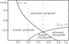Fig. 1 Up–cos θp plane. The curve in the lower right corner is the condition Lz,p = 0, expressed by Eq. (11), which divides prograde orbits (upwards and to the left of the curve) from retrograde orbits. The other line is the parabolic condition, separating elliptical orbits (on the left of the line) from the hyperbolic ones (on the right). For the meaning of the red dots, see the text.

2.3 The b-plane

We now determine the conditions that enable inclination flipping in the RC3D3BP, using results from Valsecchi et al. (2000, 2003, 2018). We consider the b-plane, namely the plane perpendicular to the incoming asymptote of the planetocentric hyperbola on which the small body moves when near the planet (Kizner 1961; Valsecchi et al. 2003; Farnocchia et al. 2019); the velocity vector U_p is directed along the incoming asymptote of the hyperbola, and crosses the b-plane in a point of coordinates ξ, ζ.

These are chosen so that (Valsecchi et al. 2003, 2018):

• the coordinate ξ = ξ(a, e, i, ω, f_b) is the local minimum of the distance between the orbits of the small body and the planet (Bowell & Muinonen 1994; Gronchi 2005; Wiśniowski & Rickman 2013), the so-called Minimum Orbit Intersection Distance (MOID);

• the coordinate ζ = ζ(a, e, i, Ω, ω, f_b,λ_p) is related to the timing of the encounter. In the above expressions, a, e, i, Ω, and ω are the elements of the pre-encounter small body orbit, f_b is the small body true anomaly, and λ_p is the longitude of the planet, both evaluated at the crossing of the b-plane.

According to Valsecchi et al. (2000; 2003), the locus of the b-plane points, leading to a post-encounter orbit with a given semi-major axis a′, is a circle whose radius and position of the centre are simple functions of the pre-encounter orbit; in our case, we are interested in the circle for a′ = a*, namely for θ′_p = θ*_p, centred in:

$$\begin{array}{cc}\xi =0& \zeta =D_{\text{p}}^{*},\end{array}$$(12)

of radius |R*_p|, with D*_p, R*_p given in units of a_p by:

$$\begin{array}{cc}{D}_{\text{p}}^{*}=\frac{c_{\text{p}}\sin {\theta }_{\text{p}}}{\cos {\theta }_{\text{p}}^{*}-\cos {\theta }_{\text{p}}}& R_{\text{p}}^{*}=\frac{c_{\text{p}}\sin {\theta }_{\text{p}}^{*}}{\cos {\theta }_{\text{p}}^{*}-\cos {\theta }_{\text{p}}},\end{array}$$(13)

where

$$c_{\text{p}}=\frac{m_{\text{p}}}{m_{\odot }{U}_{\text{p}}^2},$$(14)

with m_p and m_⊙ being, respectively, the masses of the planet and of the Sun. It is important to note that c_p, D*_p, and R*_p are all expressed in the natural units of the restricted three-body problem, that is as fractions of the heliocentric distance of the planet; if one wants them expressed in, say, astronomical units, they must be multiplied by a_p expressed in au.

Taking into account Eq. (11), we can rewrite the above expressions as:

$$\begin{array}{cc}{D}_{\text{p}}^{*}=\frac{c_{\text{p}}{U}_{\text{p}}\sin {\theta }_{\text{p}}}{1+U_{\text{p}}\cos {\theta }_{\text{p}}}& R_{\text{p}}^{*}=\frac{c_{\text{p}}\sqrt{U_{\text{p}}^2-1}}{1+U_{\text{p}}\cos {\theta }_{\text{p}}}.\end{array}$$(15)

The circle characterized by the above parameters is the frontier of the b-plane region in which the inclination flip occurs; the flip takes place for any point in the interior of the circle, which can be considered an ‘inclination-flip-gateway’. However, depending on the values of the quantities in Eq. (15), it may be that the occurrence of the flip is prevented by a collision with the planet.

Geometrically, this depends on the size and relative placement of:

• the circle representing the planet cross-section, centred in (0, 0), of radius

  $$b_{\text{p}}=\frac{r_{\text{p}}}{a_{\text{p}}}\sqrt{1+\frac{a_{\text{p}}{c}_{\text{p}}}{2r_{\text{p}}}},$$(16)

  where b_p is the impact parameter corresponding to a grazing encounter⁶ and r_p is the physical radius of the planet (Valsecchi et al. 2003),

• the inclination-flip-gateway circle centred in (0, D*_p), of radius |R*_p|, with D*_p, R*_p given by Eq. (15).

Since the numerators of Eq. (13) are always positive, D*_p and R*_p have always the same sign; thus, there are four cases for the relative placement of the two circles:

• for |D*_p| > |R*_p| and b_p < |D*_p − R*_p|, the two circles do not intersect;

• for |D*_p| < |R*_p| and b_p < |D*_p − R*_p|, the planet cross-section is fully within the inclination-flip-gateway circle, so that the area of the former has to be subtracted from the latter in order to obtain the cross-section of the inclination flip;

• for b_p > |D*_p + R*_p| the inclination-flip-gateway circle is fully within the planet cross-section, so that collision with the planet negates the possibility of inclination flip;

• finally, for b_p > |D*_p − R*_p| the two circles intersect, so that a part of the planet cross-section must be subtracted from the inclination flip cross-section.

2.4 Probabilities

Valsecchi et al. (2018) showed that varying ξ on the b-plane of an encounter is equivalent to varying ω in the initial conditions, and varying ζ is equivalent to varying M − λ_p, where M is the mean anomaly and λ_p is the longitude of the planet, both evaluated at a given time prior to the encounter. Furthermore, they showed that, keeping the value of M fixed at the given time, then small values of ξ, ζ can be mapped linearly onto the δω-δλ_p plane. The quantities δω and δλ_p are small displacements from the values of ω and λ_p that correspond to crossing the b-plane exactly in ξ = 0, ζ = 0.

The expressions for δω and δλ_p are (see Appendix A for details):

$$\delta \omega =-\frac{\sqrt{{\left(1+U_{\text{p}}\cos {\theta }_{\text{p}}\right)}^2+U_{\text{p}}^2{\sin }^2{\theta }_{\text{p}}{\cos }^2{\varphi }_{\text{p}}}}{U_{\text{p}}sin{\theta }_{\text{p}}sin{\varphi }_{\text{p}}\cos {\varphi }_{\text{p}}}·\xi$$(17)

$$\delta {\lambda }_{\text{p}}=-\frac{1+U_{\text{p}}\cos {\theta }_{\text{p}}{\sin }^2{\varphi }_{\text{p}}}{U_{\text{p}}\sin {\theta }_{\text{p}}\sin {\varphi }_{\text{p}}cos{\varphi }_{\text{p}}}·\xi +\frac{1}{\sin {\theta }_{\text{p}}}·\zeta ,$$(18)

where:

$$\sin {\varphi }_{\text{p}}=\frac{\sin f_{\text{b}}}{\left|\sin f_{\text{b}}\right|}·\frac{\sqrt{2-\frac{a_{\text{p}}}{a}-\frac{a\left(1-e^2\right)}{a_{\text{p}}}}}{U_{\text{p}}\sin {\theta }_{\text{p}}}$$(19)

$$\cos {\varphi }_{\text{p}}=\frac{\cos \left(\omega +f_{\text{b}}\right)}{\left|\cos \left(\omega +f_{\text{b}}\right)\right|}·\frac{\sqrt{\frac{a\left(1-e^2\right)}{a_{\text{p}}}}\sin i}{U_{\text{p}}\sin {\theta }_{\text{p}}}.$$(20)

From Eqs. (17) and (18) it is possible to re-derive Öpik’s classical expression for the probability of collision (Öpik 1976); this was carried out by Valsecchi et al. (2018), and is also described in Appendix B.

In the present case, provided that both |D*_p| ≪ 1 and |R*_p| ≪ 1, we can substitute s in Eq. (B.4) with R*_p from Eq. (15), obtaining (for details, see Appendix B):

$$p=\frac{c_{\text{p}}^2\left(U_{\text{p}}^2-1\right)}{\pi \sin i\sin {\theta }_{\text{p}}\left|\sin {\varphi }_{\text{p}}\right|{\left(1+U_{\text{p}}\cos {\theta }_{\text{p}}\right)}^2}.$$(21)

3 Numerical checks

3.1 (5335) Damocles

To test the quantitative reliability of the theory we compared its predictions with the results of numerical computations done in the RC3D3BP, following the method presented in Sect. 4 of Valsecchi et al. (2018). We selected two asteroids, one prograde and one retrograde, and for both of them we iteratively found the initial conditions that led to a post-encounter orbit with L′_z,p = 0; in addition, we looked for the initial conditions that led to a planetocentric perigee equal to the physical radius of the planet encountered. If the theory is quantitatively correct, then the b-plane points found numerically should be located on, or very close to, the analytically computed circles for L′_z,p = 0 and for collision with the planet, respectively.

The first check was carried out with (5335) Damocles, the namesake of the Damocloids, discovered in 1991. The orbital elements of Damocles, as well as its values of T_p and U_p with respect to the four outer planets, are given in the first line of Table 1.

Damocles has values of T_J, T_S, and T_U that enable a flip to retrograde motion as a consequence of an encounter with the respective planet; however, the current values of its MOIDs with Jupiter and Saturn are greater than 3 au, while its current MOID with Uranus is 0.31 au, allowing moderately close encounters with this planet⁷.

In order to meaningfully analyse encounters with, say, Saturn, we should compute the secular evolution of Damocles up to the epoch in which its MOID with respect to Saturn becomes small, and use the values of e and i corresponding to that epoch, since they are in principle quite different from the current values (Vokrouhlický et al. 2012). On the other hand, given the rather small current MOID with respect to Uranus, it makes sense to use the current orbit of Damocles and simulate an encounter with Uranus.

The initial conditions were selected as follows:

• our fictitious Damocles has a, e, and i given in Table 1, and Ω = 0°, M = 0°;

• the mass of Uranus is m_U = m_⊙/22903;

• Uranus moves on a circular orbit of radius 19.19 au.

We then used an iterative procedure to find the values of the argument of perihelion of Damocles and of the longitude of Uranus at the start of the integration such that Damocles encounters Uranus, and actually crosses the b-plane extremely close to ξ = 0, ζ = 0; the values found are ω₀ = 167°.856 8 and λ_U0 = 234°.875.

We then set up a double loop, the outer one on ω and the inner one on λ_U, and computed the orbital evolution in the RC3D3BP for 15 000 days, using the RA15 integrator (Everhart 1985). A close encounter with Uranus takes place within 11 000 days, and we stored the planetocentric coordinates and velocity components at the closest approach of each simulated Damocles. With appropriate rescaling and rotations, given in the Appendix of Valsecchi et al. (2018), we determined the values of ξ and ζ corresponding to the b-plane crossing of the incoming asymptote of the uranocentric hyperbola describing the motion of Damocles at the closest approach, and recorded those corresponding, as said before, to post-encounter L′_Uz = 0 and to collision with Uranus.

Figure 2 shows the results, both in the b-plane and in the plane ω-λ_U. As it is possible to see, the analytical theory turns out to be quite accurate. It is also noticeable that, although the flip to retrograde motion is possible as a consequence of an encounter with Uranus, its cross-section is smaller than that of a collision with the planet. In fact, the gravitational radius of Uranus b_U, according to Eq. (16), in this case is 3.29r_U, where r_U is the physical radius of the planet, while the radius of the b-plane circle for L′_Uz = 0 is 2.29r_U. According to Eq. (B.4), the probability per Damocles revolution of a collision with Uranus is 6.5 × 10⁻¹⁰, while the probability of flipping to a retrograde orbit is 3.1 × 10⁻¹⁰.

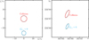Fig. 2 Conditions leading to inclination flip and to collision for an encounter of (5335) Damocles with Uranus. Left: b-plane circles corresponding to post-encounter L′Uz = 0 (cyan) and to collision with Uranus (red); the black dots come from the numerical check described in the text. Right: corresponding ellipses in the space of initial conditions ω–λU; the coloured ellipses are computed with the analytical theory, the black dots come from the numerical check.

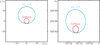Fig. 3 Conditions leading to inclination flip and to collision for an encounter of 2000 DG8 with Saturn. Left: b-plane circles corresponding to post-encounter L′Sz = 0 (cyan) and to collision with Saturn (red); the black dots come from the numerical check described in the text. Right: corresponding ellipses in the space of initial conditions ω–λS; the coloured ellipses are computed with the analytical theory, the black dots come from the numerical check.

3.2 2000 DG₈

For the second test we chose 2000 DG₈, an asteroid already in a retrograde orbit, and studied the circumstances under which its flip to a direct orbit becomes possible. The orbital elements of 2000 DG₈, and the values of T_p and U_p with respect to the four outer planets are given in the second line of Table 1. The values of T_J, T_S, and T_U enable flipping to direct motion as a consequence of an encounter with the respective planet, but it is noteworthy that an encounter with Jupiter causing the motion of 2000 DG₈ to become direct would also necessarily expel it from the Solar System. The current MOIDs of 2000 DG₈ with Jupiter and Uranus are large, but its current MOID with Saturn is only 0.096 au.

As for the initial conditions of our numerical test:

• our fictitious 2000 DG₈ has a, e, and i given in Table 1, and Ω = 0°, M = 0°;

• the mass of Saturn is m_S = m_⊙/3497.0;

• Saturn moves on a circular orbit of radius 9.537 au.

The reference values for the argument of perihelion of 2000 DG8 and for the longitude of Saturn at the start of the integration are ω₀ = 167°210 8 and λ_S0 = 332°.8362. We then proceeded as in the previous case, computing the evolution in the RC3D3BP for 15000 days; a close encounter with Saturn takes place within 12 000 d in this case, and we stored the planetocentric data at the closest approach as described before.

The results of the procedure in this case are shown in Fig. 3. The theory in this case turns out to be accurate as well. This time, the cross-section for the inclination flip is larger than that for the collision with the planet. The gravitational radius of Saturn b_S in this case is 2.40r_S, where r_S is the physical radius of the planet, while the radius of the b-plane circle for L′_Sz = 0 is 8.13r_S. However, in this case the circle corresponding to the collision is fully contained in that for L′_Sz = 0, so that one has to subtract the cross-section for collision from the cross-section for inclination flip. The probability per revolution of 2000 DG₈ colliding with Saturn is 8.1 × 10⁻⁹, while the probability of flipping to a prograde orbit, after subtracting the probability of collision, turns out to be 8.5 × 10⁻⁸.

4 Discussion

We have seen that there is a simple condition on the orbital parameters of a small body, expressed by Eq. (3), telling us whether a close encounter with a given planet can lead to an inclination flip. A number of consequences of it are discussed in the following sections.

4.1 Critical values of the semi-major axis for inclination flipping

An interesting consequence of Eq. (7) is that, if a comet or asteroid has Tisserand parameter within the appropriate range with respect to more than one planet, then its inclination flip can occur for different values of post-encounter semi-major axis, depending on the planet that is actually encountered. For example, Table 2 shows the critical values for (5335) Damocles and 2000 DG₈ with respect to each of the four outer planets. Some considerations are in order.

First, both asteroids cannot encounter Neptune on their current orbits, because their aphelia are too small; moreover, their current values of T_N would not allow an inclination flip due to an encounter with Neptune, even in the presence of such encounters. On the other hand, it must not be forgotten that encounters with a planet different from Neptune would change T_N, as described in Appendix B of Valsecchi & Manara (1997).

Second, the critical value at which the inclination flip occurs varies widely according to the planet that causes the phenomenon, as evidenced by the numbers in the table; the retrograde to prograde transition can be associated with ejection from Solar System, as would be the case if 2000 DG₈ were to encounter Jupiter, given the value of its Tisserand parameter T_J < 0.

4.2 Potentially retrograde asteroids and comets

If an asteroid is on a prograde orbit such that 0 < T_p < 2 with respect to one or more of the outer planets, and if close encounters with one of the planets for which 0 < T_p < 2 are possible, then this asteroid must be considered a ‘potentially retrograde asteroid’ (PRA), because such a close encounter could make its orbit flip to retrograde. Obviously, the same would be valid in the case of a prograde comet, that should then be considered a ‘potentially retrograde comet’ (PRC).

We saw in Sect. 2.1 that T_J < 2 can be used to separate HTCs from JFCs (Carusi et al. 1987; Levison & Duncan 1994), isotropic comets from ecliptic comets (Levison 1996), and Damocloids from the other Centaurs (Jewitt 2005). The above definitions of PRCs and PRAs can be viewed as a generalization to all the outer planets of the classification criterion just mentioned.

4.3 Limitations and advantages of the use of T_p

In the real world, T_p is not strictly conserved due to eccentricities and inclinations of the planets (Carusi et al. 1995) and due to close encounters with other planets than the one under consideration (Valsecchi & Manara 1997). On the other hand, T is generally better conserved compared to the osculating orbital elements, as shown by the numerical integrations by Levison & Duncan (1994).

That being said, it is still useful to consider the value of T_p, if we take into account results coming from the analytical theory of close encounters, such as those described in Sect. 2.4. In fact, the theory can quickly give order of magnitude estimates of the probability of orbital flip at close encounter, without the need to resort to a slow, numerical Monte Carlo approach, especially if the probability sought for is small.

5 Conclusions

In the framework of the analytical theory of close encounters (Valsecchi et al. 2000, 2003) we have identified the condition on the Tisserand parameter that allows the inclination flipping prograde ↔ retrograde of the orbit of a small Solar System body as a consequence of a close planetary encounter. This was carried out by analytically computing the b-plane region in which the small body has to pass in order to achieve the flip. Then, exploiting the correspondence between the b-plane and the ω–λ_p plane (Valsecchi et al. 2005, 2018), we have shown how to compute the probability of such an outcome.

We tested the predictions of the theory against numerical integrations in the restricted, circular, three-dimensional three-body problem, showing good agreement. Using the theory, the b-plane region leading to inclination flip can, in turn, be easily compared to the regions leading to other orbital outcomes of interest, such as planetary collision and ejection from the Solar System.

Appendix A From the b-plane to the ω-λ_p plane

We hereafter follow Valsecchi et al. (2005) and derive expressions linking small displacements in the b-plane to small displacements in a suitably chosen pair of orbital elements. In the RC3D3BP, we consider a close encounter between a small body on an orbit of given a e, and i, and a planet on an orbit of radius 1; in this setup, Ω plays the role of an ignorable coordinate, and the parameters that can be varied in the initial conditions are ω and the relative phase between the planet and the small body M − λ_p, evaluated at a certain time.

At the time of a collision, the small body and the planet are co-located. The planet is at longitude λ_pc, the small body is at heliocentric distance:

$$r_c=1=\frac{a\left(1-e^2\right)}{1+e\cos f_c},$$

where f_c is the true anomaly at collision.

Then, in a reference frame X-Y-Z centred on the planet, with the Sun at unit distance on the negative X-axis and the Y-axis in the direction of the motion of the planets, small first-order displacements in X, Y, Z can be expressed as (Valsecchi 2006):

$$\begin{array}{lll}X\hfill & =\hfill & r-1\hfill \\ Y\hfill & =\hfill & \text{Ω}-{\lambda }_{\text{p}}+\arctan \left[\cos i\tan \left(\omega +f_c\right)\right]\hfill \\ Z\hfill & =\hfill & \sin i\sin \left(\omega +f_c\right),\hfill \end{array}$$

with |r − r_c| << 1, |λ_p − λ_pc| << 1. We pass from the coordinates in the X-Y-Z frame to the b-plane coordinates with the expressions (Valsecchi 2006):

$$\begin{array}{lll}\xi \hfill & =\hfill & X\cos {\varphi }_{\text{p}}-Z\sin {\varphi }_{\text{p}}\hfill \\ \zeta \hfill & =\hfill & \left(X\sin {\varphi }_{\text{p}}+Z\cos {\varphi }_{\text{p}}\right)\cos {\theta }_{\text{p}}-Y\sin {\theta }_{\text{p}},\hfill \end{array}$$

with θ_p, ϕ_p given by Eqs. 9, 10, 19, and 20.

The partial derivatives of ξ, ζ with respect to ω, λ_p can be written as (Valsecchi et al. 2005):

$$\begin{array}{lll}\frac{\partial \xi }{\partial \omega }\hfill & =\hfill & \frac{\partial X}{\partial \omega }\cos {\varphi }_{\text{p}}-\frac{\partial Z}{\partial \omega }\sin {\varphi }_{\text{p}}\hfill \\ \frac{\partial \zeta }{\partial \omega }\hfill & =\hfill & \frac{\partial X}{\partial \omega }\cos {\theta }_{\text{p}}\sin {\varphi }_{\text{p}}+\frac{\partial Z}{\partial \omega }\cos {\theta }_{\text{p}}\cos {\varphi }_{\text{p}}-\frac{\partial Y}{\partial \omega }\sin {\theta }_{\text{p}}\hfill \\ \frac{\partial \xi }{\partial {\lambda }_{\text{p}}}\hfill & =\hfill & \frac{\partial X}{\partial {\lambda }_{\text{p}}}\cos {\varphi }_{\text{p}}-\frac{\partial Z}{\partial {\lambda }_{\text{p}}}\sin {\varphi }_{\text{p}}\hfill \\ \frac{\partial \zeta }{\partial {\lambda }_{\text{p}}}\hfill & =\hfill & \frac{\partial X}{\partial {\lambda }_{\text{p}}}\cos {\theta }_{\text{p}}\sin {\varphi }_{\text{p}}+\frac{\partial Z}{\partial {\lambda }_{\text{p}}}\cos {\theta }_{\text{p}}\cos {\varphi }_{\text{p}}-\frac{\partial Y}{\partial {\lambda }_{\text{p}}}\sin {\theta }_{\text{p}},\hfill \end{array}$$

where the partial derivatives of X, Y, Z with respect to ω, λ_p are:

$$\begin{array}{lll}\frac{\partial X}{\partial \omega }\hfill & =\hfill & 0\hfill \\ \frac{\partial Y}{\partial \omega }\hfill & =\hfill & \frac{1+U_p}{\sqrt{{\left(1+U_{\text{p}}\cos {\theta }_{\text{p}}\right)}^2+U_{\text{p}}^2{\sin }^2{\theta }_{\text{p}}{\cos }^2{\varphi }_{\text{p}}}}\hfill \\ \frac{\partial Z}{\partial \omega }\hfill & =\hfill & \frac{U_p\sin {\theta }_{\text{p}}\cos {\varphi }_{\text{p}}}{\sqrt{{\left(1+U_{\text{p}}\cos {\theta }_{\text{p}}\right)}^2+U_{\text{p}}^2{\sin }^2{\theta }_{\text{p}}{\cos }^2{\varphi }_{\text{p}}}}\hfill \\ \frac{\partial X}{\partial {\lambda }_{\text{p}}}\hfill & =\hfill & 0\hfill \\ \frac{\partial Y}{\partial {\lambda }_{\text{p}}}\hfill & =\hfill & -1\hfill \end{array}$$

$$\frac{\partial Z}{\partial {\lambda }_{\text{p}}}=0.$$

Substituting, we have:

$$\frac{\partial \xi }{\partial \omega }=-\frac{U_p\sin {\theta }_{\text{p}}\sin {\varphi }_{\text{p}}\cos {\varphi }_{\text{p}}}{\sqrt{{\left(1+U_{\text{p}}\cos {\theta }_{\text{p}}\right)}^2+U_{\text{p}}^2{\sin }^2{\theta }_{\text{p}}{\cos }^2{\varphi }_{\text{p}}}}$$(A.1)

$$\frac{\partial \zeta }{\partial \omega }=-\frac{\sin {\theta }_{\text{p}}\left(1+U_p\cos {\theta }_{\text{p}}{\sin }^2{\varphi }_{\text{p}}\right)}{\sqrt{{\left(1+U_{\text{p}}\cos {\theta }_{\text{p}}\right)}^2+U_{\text{p}}^2{\sin }^2{\theta }_{\text{p}}{\cos }^2{\varphi }_{\text{p}}}}$$(A.2)

$$\frac{\partial \xi }{\partial {\lambda }_{\text{p}}}=0$$(A.3)

$$\frac{\partial \zeta }{\partial {\lambda }_{\text{p}}}=\sin {\theta }_{\text{p}}.$$(A.4)

Therefore, for small displacements in the δλ_p − δω plane, the corresponding displacements in the b-plane are given by:

$$\begin{array}{lll}\left(\begin{array}{c}\xi \\ \zeta \end{array}\right)\hfill & =\hfill & \left(\begin{array}{cc}\frac{\partial \xi }{\partial \omega }& \frac{\partial \xi }{\partial {\lambda }_{\text{p}}}\\ \frac{\partial \zeta }{\partial \omega }& \frac{\partial \zeta }{\partial {\lambda }_{\text{p}}}\end{array}\right)\left(\begin{array}{c}\delta \omega \\ \delta {\lambda }_{\text{p}}\end{array}\right)\hfill \\ \hfill & =\hfill & \left(\begin{array}{cc}-\frac{U_{\text{p}}\sin {\theta }_{\text{p}}\sin {\varphi }_{\text{p}}\cos {\varphi }_{\text{p}}}{\sqrt{{\left(1+U_{\text{p}}\cos {\theta }_{\text{p}}\right)}^2+U_{\text{p}}^2{\sin }^2{\theta }_{\text{p}}{\cos }^2{\varphi }_{\text{p}}}}& 0\\ -\frac{\sin {\theta }_{\text{p}}\left(1+U_{\text{p}}\cos {\theta }_{\text{p}}{\sin }^2{\varphi }_{\text{p}}\right)}{\sqrt{{\left(1+U_{\text{p}}\cos {\theta }_{\text{p}}\right)}^2+U_{\text{p}}^2{\sin }^2{\theta }_{\text{p}}{\cos }^2{\varphi }_{\text{p}}}}& \sin {\theta }_{\text{p}}\end{array}\right)\hfill \\ \hfill & \hfill & ·\left(\begin{array}{c}\delta \omega \\ \delta {\lambda }_{\text{p}}\end{array}\right).\hfill \end{array}$$(A.5)

The determinant D of the 2 × 2 matrix is:

$$\begin{array}{lll}D\hfill & =\hfill & \left|\begin{array}{cc}\frac{\partial \xi }{\partial \omega }& \frac{\partial \xi }{\partial {\lambda }_{\text{p}}}\\ \frac{\partial \zeta }{\partial \omega }& \frac{\partial \zeta }{\partial {\lambda }_{\text{p}}}\end{array}\right|\hfill \\ \hfill & =\hfill & -\frac{U{\sin }^2{\theta }_{\text{p}}\sin {\varphi }_{\text{p}}\cos {\varphi }_{\text{p}}}{\sqrt{{\left(1+U_{\text{p}}\cos {\theta }_{\text{p}}\right)}^2+U^2{\sin }^2{\theta }_{\text{p}}{\cos }^2{\varphi }_{\text{p}}}}\hfill \end{array}$$(A.6)

The inverse relationship, provided that D is not zero, is:

$$\left(\begin{array}{c}\delta \omega \\ \delta {\lambda }_{\text{p}}\end{array}\right)=\frac{1}{D}\left(\begin{array}{cc}\frac{\partial \zeta }{\partial {\lambda }_{\text{p}}}& -\frac{\partial \xi }{\partial {\lambda }_{\text{p}}}\\ -\frac{\partial \zeta }{\partial \omega }& \frac{\partial \xi }{\partial \omega }\end{array}\right)\left(\begin{array}{c}\xi \\ \zeta \end{array}\right),$$

so that, finally, we get expressions for the linear transformation from ξ, ζ to δω, δλ_p:

$$\left(\begin{array}{c}\delta \omega \\ \delta {\lambda }_{\text{p}}\end{array}\right)=\left(\begin{array}{cc}-\frac{\sqrt{{\left(1+U_{\text{p}}\cos {\theta }_{\text{p}}\right)}^2+U_{\text{p}}^2{\sin }^2{\theta }_{\text{p}}{\cos }^2{\varphi }_{\text{p}}}}{U_{\text{p}}\sin {\theta }_{\text{p}}\sin {\varphi }_{\text{p}}\cos {\varphi }_{\text{p}}}& 0\\ -\frac{1+U_{\text{p}}\cos {\theta }_{\text{p}}{\sin }^2{\varphi }_{\text{p}}}{U_{\text{p}}\sin {\theta }_{\text{p}}\sin {\varphi }_{\text{p}}\cos {\varphi }_{\text{p}}}& \sin {\theta }_{\text{p}}\end{array}\right)\left(\begin{array}{c}\xi \\ \zeta \end{array}\right)$$(A.7)

Thus, the b-plane circles become ellipses when the corresponding initial conditions are plotted in the ω-λ_p plane, as shown in the right panels of Figs. 2 and 3.

It should be noted that in Eq. 18 and in the second row of the matrix in Eq. A.7 the signs are opposite to those of the corresponding expression in Valsecchi et al. (2018); there, it was erroneously reported the expression for δM, valid for fixed λ_p, while the computations reported were, as in the present case, for fixed M and variable λ_p. This has an effect only on the orientation of the ellipses in the right panels of Figs. 2 and 3, but does not change their areas, and thus does not change the related probabilities, as shown in the next appendix.

Appendix B From the ω-λ_p plane to probabilities

The characteristic polynomial of the linear transformation given in Eq. A.7 is:

$$0={\text{Λ}}^2-\frac{1}{D}\left(\frac{\partial \zeta }{\partial {\lambda }_{\text{p}}}+\frac{\partial \xi }{\partial \omega }\right)\text{Λ}+\frac{1}{D^2}\frac{\partial \zeta }{\partial {\lambda }_{\text{p}}}\frac{\partial \xi }{\partial \omega },$$

where we have taken into account that ∂ξ/∂λ_p = 0; the eigenvalues are:

$$\begin{array}{lll}{\text{Λ}}_1\hfill & =\hfill & -\frac{\sqrt{{\left(1+U_{\text{p}}\cos {\theta }_{\text{p}}\right)}^2+U_{\text{p}}^2{\sin }^2{\theta }_{\text{p}}{\cos }^2{\varphi }_{\text{p}}}}{U_{\text{p}}\sin {\theta }_{\text{p}}\sin {\varphi }_{\text{p}}\cos {\varphi }_{\text{p}}}\hfill \\ {\text{Λ}}_2\hfill & =\hfill & \frac{1}{\sin {\theta }_{\text{p}}}.\hfill \end{array}$$

Thus, the area of the ellipse on the δω, δλ_p plane corresponding to a small circle on the b-plane of radius r, centred in, or close to, the origin, is π|Λ₁ Λ₂|r². In fact, for the same set of a, e, i, and Ω, there are four possibilities of close encounters, and thus four b-planes, corresponding to the four possible collisions: post-perihelion, ascending node; post-perihelion, descending node; pre-perihelion, ascending node; pre-perihelion, descending node. Therefore we have to multiply that area by four. On the other hand, the area spanned by λ_p and ω is 4π².

It follows from the above considerations that the probability, per sidereal revolution, that at a close encounter the small body will hit the b-plane within a small circle of radius r, centred in or close to the origin, is:

$$\begin{array}{lll}{p}_r\left(b\right)\hfill & =\hfill & 4·\frac{\pi \left|{\text{Λ}}_1{\text{Λ}}_2\right|r^2}{4{\pi }^2}\hfill \\ \hfill & =\hfill & \frac{r^2\sqrt{1+{\left(U_p\cos {\theta }_p\right)}^2+U_{\text{p}}^2{\sin }^2{\theta }_{\text{p}}{\cos }^2{\varphi }_{\text{p}}}}{\pi U_p{\sin }^2{\theta }_{\text{p}}\left|\sin {\varphi }_{\text{p}}\right|\left|\cos {\varphi }_{\text{p}}\right|}.\hfill \end{array}$$(B.1)

Taking into account the expression for sin i in terms of U_p,θ_p, ϕ_p (Valsecchi et al. 2018):

$$\sin i=\frac{U_{\text{p}}\sin {\theta }_{\text{p}}\left|\cos {\varphi }_{\text{p}}\right|}{\sqrt{{\left(1+U_p\cos {\theta }_{\text{p}}\right)}^2+U_{\text{p}}^2{\sin }^2{\theta }_p{\cos }^2{\varphi }_{\text{p}}},}$$(B.2)

we can rewrite Eq. B.1 as

$$p_r\left(b\right)=\frac{r^2}{\pi \sin i\sin {\theta }_{\text{p}}\left|\sin {\varphi }_{\text{p}}\right|}.$$(B.3)

This last expression is identical to the one given by Öpik for the probability per revolution of collision with a planet of target radius s (Öpik 1976):

$$p=\frac{s^{2}U}{\pi \sin i\left|U_x\right|}=\frac{s^2}{\pi \sin i\sin {\theta }_{\text{p}}\left|\sin {\varphi }_{\text{p}}\right|}.$$(B.4)

References

All Tables

All Figures

	Fig. 1 Up–cos θp plane. The curve in the lower right corner is the condition Lz,p = 0, expressed by Eq. (11), which divides prograde orbits (upwards and to the left of the curve) from retrograde orbits. The other line is the parabolic condition, separating elliptical orbits (on the left of the line) from the hyperbolic ones (on the right). For the meaning of the red dots, see the text.
In the text

Fig. 2 Conditions leading to inclination flip and to collision for an encounter of (5335) Damocles with Uranus. Left: b-plane circles corresponding to post-encounter L′Uz = 0 (cyan) and to collision with Uranus (red); the black dots come from the numerical check described in the text. Right: corresponding ellipses in the space of initial conditions ω–λU; the coloured ellipses are computed with the analytical theory, the black dots come from the numerical check.

In the text

Fig. 3 Conditions leading to inclination flip and to collision for an encounter of 2000 DG8 with Saturn. Left: b-plane circles corresponding to post-encounter L′Sz = 0 (cyan) and to collision with Saturn (red); the black dots come from the numerical check described in the text. Right: corresponding ellipses in the space of initial conditions ω–λS; the coloured ellipses are computed with the analytical theory, the black dots come from the numerical check.

In the text

References

- Bowell, E., & Muinonen, K. 1994, in Hazards due to comets and asteroids, eds. T. Gehrels, M. S. Matthews, & A. Schumann (Tucson: University of Arizona Press), 149 [Google Scholar]
- Brož, M., Morbidelli, A., Bottke, W. F., et al. 2013, A&A, 551, A117 [Google Scholar]
- Carusi, A., Kresák, Ľ., Perozzi, E., & Valsecchi, G. B. 1987, A&A, 187, 899 [NASA ADS] [Google Scholar]
- Carusi, A., Valsecchi, G. B., & Greenberg, R. 1990, Celest. Mech. Dyn. Astron., 49, 111 [Google Scholar]
- Carusi, A., Kresák, L., & Valsecchi, G. B. 1995, Earth Moon and Planets, 68, 71 [NASA ADS] [CrossRef] [Google Scholar]
- Everhart, E. 1985, in IAU Colloq. Dynamics of Comets: Their Origin and Evolution, eds. A. Carusi, & G. B. Valsecchi (D. Reidel Publishing Company) 83, 185 [NASA ADS] [CrossRef] [Google Scholar]
- Farnocchia, D., Eggl, S., Chodas, P. W., Giorgini, J. D., & Chesley, S. R. 2019, Celest. Mech. Dyn. Astron., 131, 36 [NASA ADS] [CrossRef] [Google Scholar]
- Greenberg, R., Carusi, A., & Valsecchi, G. B. 1988, Icarus, 75, 1 [NASA ADS] [CrossRef] [Google Scholar]
- Greenstreet, S., Ngo, H., & Gladman, B. 2012, Icarus, 217, 355 [CrossRef] [Google Scholar]
- Gronchi, G. F. 2005, Celest. Mech. Dyn. Astron., 93, 295 [Google Scholar]
- Jewitt, D. 2005, AJ, 129, 530 [NASA ADS] [CrossRef] [Google Scholar]
- Kizner, W. 1961, Planet. Space Sci., 7, 125 [NASA ADS] [CrossRef] [Google Scholar]
- Kresák, L. 1972a, Bull. Astron. Inst. Czech., 23, 1 [Google Scholar]
- Kresák, L. 1972b, in The Motion, Evolution of Orbits, and Origin of Comets, eds. G. A. Chebotarev, E. I. Kazimirchak-Polonskaia, & B. G. Marsden, IAU Symposium, 45, 503 [Google Scholar]
- Levison, H. F. 1996, Completing the Inventory of the Solar System, eds. T. Rettig, & J. M. Hahn, ASP. Conf. Ser., 107, 173 [NASA ADS] [Google Scholar]
- Levison, H. F., & Duncan, M. J. 1994, Icarus, 108, 18 [NASA ADS] [CrossRef] [Google Scholar]
- Lithwick, Y., & Naoz, S. 2011, ApJ, 742, 94 [NASA ADS] [CrossRef] [Google Scholar]
- Naoz, S., Li, G., Zanardi, M., de Elía, G. C., & Di Sisto, R. P. 2017, AJ, 154, 18 [NASA ADS] [CrossRef] [Google Scholar]
- Öpik, E. J. 1976, Interplanetary Encounters - Close-range Gravitational Interactions (Amsterdam: Elsevier) [Google Scholar]
- Rickman, H., Gabryszewski, R., Wajer, P., et al. 2017, A&A, 598, A110 [NASA ADS] [CrossRef] [EDP Sciences] [Google Scholar]
- Roy, A. E. 2005, Orbital Motion (Bristol: IOP Publishing) [Google Scholar]
- Tisserand, F. 1889a, Bull. Astron., Ser. I, 6, 241 [CrossRef] [Google Scholar]
- Tisserand, F. 1889b, Bull. Astron., Ser. I, 6, 289 [CrossRef] [Google Scholar]
- Valsecchi, G. B. 2006, in Dynamics of Extended Celestial Bodies and Rings, ed. J. Souchay, 682, 145 [NASA ADS] [CrossRef] [Google Scholar]
- Valsecchi, G. B. 2007, in Near Earth Objects, our Celestial Neighbors: Opportunity and Risk, eds. A. Milani, G. B. Valsecchi, & D. Vokrouhlický, IAU Symposium, 236, 17 [NASA ADS] [Google Scholar]
- Valsecchi, G. B., & Manara, A. 1997, A&A, 323, 986 [NASA ADS] [Google Scholar]
- Valsecchi, G. B., Jopek, T. J., & Froeschlé, C. 1999, MNRAS, 304, 743 [NASA ADS] [CrossRef] [Google Scholar]
- Valsecchi, G. B., Milani, A., Gronchi, G. F., & Chesley, S. R. 2000, Celest. Mech. Dyn. Astron., 78, 83 [NASA ADS] [CrossRef] [Google Scholar]
- Valsecchi, G. B., Milani, A., Gronchi, G. F., & Chesley, S. R. 2003, A&A, 408, 1179 [NASA ADS] [CrossRef] [EDP Sciences] [Google Scholar]
- Valsecchi, G. B., Rossi, A., Milani, A., & Chesley, S. R. 2005, in IAU Colloq. Dynamics of Populations of Planetary Systems, eds. Z. Kneževic & A. Milani, 197, 249 [NASA ADS] [Google Scholar]
- Valsecchi, G. B., Alessi, E. M., & Rossi, A. 2018, Celest. Mech. Dyn. Astron., 130, 8 [NASA ADS] [CrossRef] [Google Scholar]
- Vokrouhlický, D., Pokorný, P., & Nesvorný, D. 2012, Icarus, 219, 150 [CrossRef] [Google Scholar]
- Wiśniowski, T., & Rickman, H. 2013, Acta Astron., 63, 293 [NASA ADS] [Google Scholar]
For a discussion of the Tisserand parameter see Sect. 2.
From (5335) Damocles, the first asteroid discovered in such an orbit.
It should be noted that bp, the same as cp, D*p, and R*p, is expressed as a fraction of the heliocentric distance of the planet.
The values of the MOIDs used here come from the Minor Planet Center, https://minorplanetcenter.net/db_search