© M. Harsoula et al. 2022

1. Introduction

There are two main theories that prevail nowadays concerning the building blocks of the spiral arms in galaxies. In the case of grand design galaxies, the “density wave” theory remains a valid dynamical model with which the spiral structure of many disk galaxies can be described. The density wave theory fits the description of spiral arms better when the spiral amplitude does not exceed a value of 10%–20% over a few pattern rotations. This theory was first developed by Lindblad (1940, 1961), and it was extended by Lin & Shu (1964, 1966). Lindblad (1955) pioneered the orbital description of spiral density waves. In the density wave theory, the periodic orbits are close to precessing ellipses that support the shape of the spiral structure. Many papers have studied these periodic orbits, in models of grand design galaxies. It has been shown that these orbits can collaborate so that the imposed model matches with the response model of spiral arms (see Contopoulos 1970, 1971, 1975; Berman & Mark 1977; Monet & Vandervoort 1978; Contopoulos & Grosbøl 1986; Patsis et al. 1991; Harsoula et al. 2021).

On the other hand, in the case of barred spiral galaxies, where the perturbation of the bar component is large enough and introduces chaos near corotation, the prevailing theory for the spiral arms is the “manifold theory” (Danby 1965; Voglis et al. 2006; Romero-Gomez et al. 2006, 2007; Tsoutsis et al. 2008, 2009; Athanassoula et al. 2009a,b; Athanassoula 2012; Harsoula et al. 2016). This theory predicts bisymmetric spirals emanating from the ends of galactic bars as a result of the outflow of matter connected with the unstable dynamics around the bar’s Lagrangian points L₁ and L₂. In this case the spiral arms are supported by chaotic orbits having initial conditions along the unstable manifolds emanating from L₁ and L₂. More recently, Efthymiopoulos et al. (2020) found empirically that the manifold spirals, which are computed in an N-body simulation by momentarily “freezing” the potential and making all calculations in a frame that rotates with the instantaneous pattern speed of the bar, reproduce the time-varying morphology of the N-body spirals rather well. In that simulation it was also found that multiple patterns are demonstrably present. Observations of barred spiral galaxies have shown that the existence of two different pattern speeds for the spiral arms and the bar is a very possible scenario (Moore & Gottesman 1995; Boonyasait et al. 2005; Meidt et al. 2009; Speights & Westpfahl 2012; Speights & Rooke 2016; Font et al. 2019). The same conclusion emerges from simulations (Sellwood & Sparke 1988; Rautiainen & Salo 1999; Quillen 2003; Quillen et al. 2011; Roca-Fàbrega et al. 2013; Font et al. 2014). A brief review of the different methods used to determine the pattern speeds of the Galactic bar and spiral arms of the Milky Way was given in Gerhard (2011). In most cases the ratio of the two pattern speeds is 1:2 or 1:3, with the spiral arms always having the lowest value. In Efthymiopoulos et al. (2020) it has been shown that, in a Milky Way-like model with two different pattern speeds for the bar and the spiral arms, the manifold theory can still be valid if the spiral potential is considered as a perturbation of the bar’s potential. As a consequence, the unstable Lagrangian points L₁ and L₂ of the pure bar model are continued in the full model as periodic orbits, or as epicyclic “Lissajous-like” unstable orbits.

In the present paper we reverse the idea of Efthymiopoulos et al. (2020) and we consider the potential of the bar as a perturbation of the spiral potential. An important quantity in this connection is the Q-strength, which gives an estimate of the relative importance of the bar’s and the spirals’ non-axisymmetric force perturbations. The Q-strength at fixed radius r (e.g., Buta et al. 2009) is defined for the bar as

$$\begin{array}{c}\hfill Q_{\mathrm{b}}(r)=\frac{F_{\mathrm{b},\mathrm{t}}^{\max }(r)}{⟨F(r)⟩},\end{array}$$(1)

where $F_{\mathrm{b},\mathrm{t}}^{\max }(r)$ is the maximum tangential force generated by the potential term of the bar V_bar at the distance r, with respect to all azimuths ϕ. Moreover, ⟨F(r)⟩ is the average radial force at the same distance, with respect to ϕ, generated by the total potential V_ax + V_bar + V_sp. The Q-strength of the bar is always much larger than the one of the spiral arms (Buta et al. 2005, 2009; Durbala et al. 2009). However, the Q-strength alone is not sufficient to state the importance of the bar’s perturbation in relation to the spiral perturbation. In the case where the bar rotates much faster that the spiral arms, an observer rotating with the spiral arms would see the bar as a kind of a bulge (an average axisymmetric component). In such a case, the potential of the bar can be considered as a perturbation of the potential of the spiral arms. Therefore, in such a case, a generalization of the density wave theory can be considered. Under this assumption, we construct a semianalytical algorithm, with the help of a normal form algorithm, with the aim of eliminating time dependence from the Hamiltonian (due to the difference in the pattern speeds). Then, in this new Hamiltonian, the precessing ellipses that support the spiral structure in the case of grand design galaxies is transformed into quasiperiodic orbits forming ellipses with a certain thickness. When we superimpose all of them at different energy levels, we can again extract a spiral density wave by calculating the isodensities, using an image processing method described below (Sect. 3.2).

This paper contains the following: In Sect. 2 we give a description of the galactic model that we use in our study. In Sect. 3 we quote the normal form construction of the Hamiltonian corresponding to the galactic model and describe the way of locating the stable periodic orbits that are responsible for the spiral density way. We also plot these orbits in the old variables before the normal form transformation in order to see how the precessing ellipses have been deformed and if we can still detect a spiral density wave. In Sect. 4 we make a parametric study in order to see how the mass and the pattern speed of the bar affects the outcome of the spiral density wave derived from the procedure described in Sect. 3. Finally, in Sect. 5 we summarize the conclusions of our study.

2. The model

We consider a model of a Milky Way-like spiral galaxy that contains a combination of a bar, an axisymmetric, and a spiral potential used in Pettitt et al. (2014):

$$\begin{array}{c}\hfill V=V_{\mathrm{ax}}+V_{\mathrm{sp}}+V_{\mathrm{bar}}.\end{array}$$(2)

The axisymmetric potential V_ax is composed of a disk, a halo, and the axisymmetric part of the bar’s potential, which plays the role of a central bulge:

$$\begin{array}{c}\hfill V_{\mathrm{ax}}=V_{\mathrm{d}}(r)+V_{\mathrm{h}}(r)+V_{{\mathrm{b}}_0}(r).\end{array}$$(3)

For the disk potential V_d, we use a Miyamoto–Nagai model (Miyamoto & Nagai 1975) given by the relation

$$\begin{array}{c}\hfill V_{\mathrm{d}}=\frac{-G{M}_{\mathrm{d}}}{\sqrt{r^2+{(a_{\mathrm{d}}+\sqrt{z^2+b_{\mathrm{d}}^2})}^2}},\end{array}$$(4)

where M_d = 8.56 × 10¹⁰ M_⊙ is the total mass of the disk, a_d = 5.3 kpc, and b_d = 0.25 kpc. In order to have a 2D disk model, we take z = 0 and $r=\sqrt{x^2+{\mathit{y}}^2}$.

The halo potential is a γ-model (Dehnen 1993) with parameters as in Pettitt et al. (2014),

$$\begin{array}{c}\hfill V_{\mathrm{h}}=\frac{-G{M}_{\mathrm{h}(\mathrm{r})}}{r}-\frac{-G{M}_{\mathrm{h},0}}{\gamma r_{\mathrm{h}}}{[-\frac{\gamma }{1+{(r/r_{\mathrm{h}})}^{\gamma }}+ln{(1+\frac{r}{r_{\mathrm{h}}})}^{\gamma }]}_{\mathrm{r}}^{r_{\mathrm{h},\max }},\end{array}$$(5)

where r_h, max = 100 kpc, γ = 1.02, M_h, 0 = 10.7 × 10¹⁰ M_⊙, and M_h(r) is given by the function:

$$\begin{array}{c}\hfill M_{\mathrm{h}(\mathrm{r})}=\frac{M_{\mathrm{h},0}{(r/r_{\mathrm{h}})}^{\gamma +1}}{1+{(r/r_{\mathrm{h}})}^{\gamma }}.\end{array}$$(6)

The spiral potential is given by the value V_sp (for z = 0) of the 3D logarithmic spiral model V_sp(r, ϕ, z) introduced by Cox & Gomez (2002; see Formula (19) in Efthymiopoulos et al. 2020):

$$\begin{array}{c}\hfill V_{\mathrm{sp}}=4\pi G{h}_z{\rho }_{0}G(r)exp(-\left(\frac{r-r_0}{R_{\mathrm{s}}}\right))\frac{C}{\mathit{KB}}cos\left[2(\phi -\frac{ln(r/r_0)}{tan(\alpha )})\right],\end{array}$$(7)

where

$$\begin{array}{c}\hfill K=\frac{2}{r|sin(\alpha )|},B=\frac{1+K{h}_z+0.3{(K{h}_z)}^2}{1+0.3K{h}_z},\end{array}$$(8)

and C = 8/(3π), h_z = 0.18 kpc, r₀ = 8 kpc, R_s = 7 kpc, and a = −13° is the pitch angle of the spiral arms. The function G(r) plays the role of a smooth envelope determining the radius beyond which the spiral arms are important. We adopt the form G(r) = b − carctan(R_s0 − r), with R_s0 = 6 kpc, b = 0.474, and c = 0.335. The spiral density is ρ₀ = 15 × 10⁷ M_⊙ kpc⁻³ in the model under study. This value of the spiral density is chosen so as to yield a spiral F-strength value of 15%, consistent with those reported in the literature for the case of an intermediate spiral perturbation (see Patsis et al. 1991; Grosbøl et al. 2004) for grand design galaxies, and Sarkar & Jog (2018) and Pettitt et al. (2014) for the Milky Way. The F-strength value is given by the ratio of the maximum total force of the spiral perturbation over the radial force of the axisymmetric background:

$$\begin{array}{c}\hfill F_{\mathrm{all}}(r)=\frac{\langle F_{\mathrm{sp}}(r)\rangle }{F_{\mathrm{r}}(r)}=\frac{{\langle \sqrt{{\left(\frac{1}{r}\frac{\partial V_{\mathrm{sp}}}{\partial \phi }\right)}^2+{\left(\frac{\partial V_{\mathrm{sp}}}{\partial r}\right)}^2}\rangle }_{\max }}{\frac{\partial V_{\mathrm{ax}}}{\partial r}}\end{array}$$(9)

(see Fig. 1 and corresponding text of Harsoula et al. 2021 for a detailed explanation of the role of the F-strength value).

The bar’s potential potential is as in Long & Murali (1992):

$$\begin{array}{c}\hfill V_{\mathrm{b}}=\frac{G{M}_{\mathrm{b}}}{2a}ln\left(\frac{x-a+T_{-}}{x+a+T_{+}}\right),\end{array}$$(10)

with

$$\begin{array}{c}\hfill T_{\pm }=\sqrt{{(a\pm x)}^2+y^2+{(b+\sqrt{c^2+z^2})}^2},\end{array}$$(11)

where M_b is the mass of the bar. In our study we use three different values of M_b, namely M_b = (6.25,  3,  1)×10¹⁰ M_⊙, where M_⊙ is the solar mass, a = 5.25 kpc, b = 2.1 kpc, and c = 1.6 kpc. The values of a and b set the bar’s length along the major and minor axes in the disk plane (x and y, respectively), while c sets the bar’s thickness in the z-axis (see Gerhard 2002; Rattenbury et al. 2007; Cao et al. 2013). These values are chosen so as to bring the bar’s corotation (for Ω_b = 45 km s⁻¹ kpc⁻¹) to the value (specified by the L_1, 2 points distance from the center) R_L1, 2 = 5.4 kpc. Assuming corotation to be at 1.2 − 1.3 times the bar length, as seen in the literature, the latter turns to be about 4 Kpc with the adopted parameters. We set z = 0, because we deal with the 2D model, and finally, Eq. (10) in polar coordinates (r, θ), in the inertial frame of reference, takes the form

$$\begin{array}{l}{V}_{\text{b}}(r,\theta )=\frac{G{M}_{\text{b}}}{2a}\\ \times \ln \left(\frac{r\cos (\theta )-a+\sqrt{{(r\cos (\theta )-a)}^2+{(b+c)}^2+r^2{\sin }^2(\theta )}}{r\cos (\theta )+a+\sqrt{{(r\cos (\theta )+a)}^2+{(b+c)}^2+r^2{\sin }^2(\theta )}}\right).\end{array}$$(12)

We now make a Taylor expansion of Eq. (12) with respect to cos(θ) and rewrite the bar’s potential as the sum of cos(mθ) terms, where m = 0, 2, 4, 6. Then, Eq. (12) takes the form

$$\begin{array}{l}{V}_{\text{b}}(r,\theta )=V_{\text{b0}}(r)+{\displaystyle \sum _{m=2}^6{V}_{\text{bm}}}(r,\theta )\\ =A_{\text{b}0}(r)+A_{\text{b2}}(r)\cos (2\theta )+A_{\text{b4}}(r)\cos (4\theta )+A_{\text{b6}}(r)\cos (6\theta ).\end{array}$$(13)

The bar’s and the spiral’s potential, in the inertial frame of reference and in polar coordinates (r, θ), are given by the following relations:

$$\begin{array}{c}\hfill V_{{\mathrm{b}}_{\mathrm{in}}}=V_{\mathrm{b}}(r,\theta -{\mathrm{\Omega }}_{\mathrm{b}}t),V_{{\mathrm{sp}}_{\mathrm{in}}}=V_{\mathrm{sp}}(r,\theta -{\mathrm{\Omega }}_{\mathrm{sp}}t),\end{array}$$(14)

where Ω_b is the pattern speed of the bar and Ω_sp is the pattern speed of the spiral arms in the inertial frame of reference. The Hamiltonian of the total potential, in the rotating frame of reference of the spiral potential, is then written in the form

$$\begin{array}{c}\hfill H_{\mathrm{in}}(r,f,f_2)=\frac{p_{\mathrm{r}}^2}{2}+\frac{p_{\mathrm{f}}^2}{2r^2}-{\mathrm{\Omega }}_{\mathrm{sp}}{p}_{\mathrm{f}}+V_{\mathrm{ax}}(r)\\ \hfill +{\displaystyle \sum _{m=2}^6}{V}_{\mathrm{bm}}(r,f+f_2)+V_{\mathrm{sp}}(r,f)+\mathrm{\Delta }\mathrm{\Omega }{J}_2,\end{array}$$(15)

where p_r is the radial velocity per unit mass, p_f is the angular momentum of the unit mass in the rest frame of reference, f = θ − Ω_spt, f₂ = ΔΩt = (Ω_sp − Ω_b) t, and J₂ is the canonically conjugate action of the angle f₂. The axisymmetric part of the potential V_ax(r), as given by Eq. (3), includes the axisymmetric part of the bar’s potential V_b0(r), while the non-axisymmetric part of the bar’s potential V_bm(r, f + f₂) includes, in a first approximation, only the m = 2 terms of the bar’s potential, in order to facilitate the construction of the normal form:

$$\begin{array}{c}\hfill V_{{\mathrm{b}}_2}(r,f+f_2)=A_{{\mathrm{b}}_2}(r)cos(2(f+f_2)).\end{array}$$(16)

3. Normal form construction

We now make a Taylor expansion of the bar’s potential V_b2(r, f, f₂) around the radius of the circular orbit r_c and the corresponding angular momentum p_c, up to the second order, making the following replacements:

$$\begin{array}{c}\hfill r=r_{\mathrm{c}}+\delta r,p_{\mathrm{f}}=p_{\mathrm{c}}+J_{\mathrm{u}},\end{array}$$(17)

where δr is a small perturbation of the radius in relation to the radius of the circular orbit r_c and J_u is a small perturbation of the angular momentum in relation to the angular momentum of the circular orbit p_c. Finally, we make a canonical transformation in action-angle variables (δr, p_r)→(J_r, f_r):

$$\begin{array}{c}\hfill \delta r=\sqrt{2J_{\mathrm{r}}/{\kappa }_{\mathrm{c}}}sin{f}_{\mathrm{r}},p_{\mathrm{r}}=\sqrt{2J_{\mathrm{r}}{\kappa }_{\mathrm{c}}}cos{f}_{\mathrm{r}},\end{array}$$(18)

where k_c(r_c) is the epicyclic frequency at r = r_c, given by the relation

$$\begin{array}{c}\hfill {\kappa }_{\mathrm{c}}=\sqrt{\frac{{\mathrm{d}}^2{V}_{\mathrm{ax}}(r_{\mathrm{c}})}{\mathrm{d}{r}_{\mathrm{c}}^2}+\frac{3}{r_{\mathrm{c}}}\frac{\mathrm{d}{V}_{\mathrm{ax}}(r_{\mathrm{c}})}{\mathrm{d}{r}_{\mathrm{c}}}},\end{array}$$(19)

Moreover, p_c is related to the angular velocity Ω(r_c) of the star with the relation $p_{\text{c}}=\mathrm{\Omega }(r_{\text{c}})r_{\text{c}}^2$. The angular velocity Ω(r_c), under the action of the axisymmetric potential only, is given by the relation

$$\begin{array}{c}\hfill {\mathrm{\Omega }}_{\mathrm{c}}=\sqrt{\frac{1}{r_{\mathrm{c}}}\frac{\mathrm{d}{V}_{\mathrm{ax}}(r_{\mathrm{c}})}{\mathrm{d}{r}_{\mathrm{c}}}}.\end{array}$$(20)

Then, the Hamiltonian (15) takes the following form:

$$\begin{array}{cc}& H_{\mathrm{new}}(J_{\mathrm{u}},J_{\mathrm{r}},J_2,f,f_{\mathrm{r}},f_2)=H_{\mathrm{c}}+\mathrm{\Delta }\mathrm{\Omega }{J}_2+{\kappa }_{\mathrm{c}}{J}_{\mathrm{r}}+(\mathrm{\Omega }(r_{\mathrm{c}})-{\mathrm{\Omega }}_{\mathrm{sp}})Ju\hfill \\ \hfill & +{\displaystyle \sum _{m_1,m_2,m_3}}{a}_{m_1,m_2,m_3}{(J_{\mathrm{r}})}_{sin}^{cos}(m_{1}f+m_2{f}_2+m_3{f}_{\mathrm{r}}),\hfill \end{array}$$(21)

where m₁, m₂, m₃ can take the values 0, ±1, ±2. The notation ${}_{sin}^{cos}(m_{1}f+m_2{f}_2+m_3{f}_{\mathrm{r}})$ in the summation of Eq. (21) means that there are both terms with sin(m₁f + m₂f₂ + m₃f_r) and cos(m₁f + m₂f₂ + m₃f_r). ΔΩ = Ω_sp − Ω_b and H_c is a constant term that can be omitted.

We now want to construct a normal form of the Hamiltonian (21) in order to eliminate the terms that contain the angle f₂ = ΔΩt and make the Hamiltonian nonautonomous (for a tutorial on the normal form construction, see Efthymiopoulos 2012). We introduce a formal notation to account for this consideration: in front of every term in Eq. (21), we introduce a factor, λ^s, hereafter called the “book-keeping parameter”, which is a constant with a numerical value equal to λ = 1, while s is a positive integer exponent whose value, for every term in Eq. (21), is selected so as to reflect our consideration regarding the order of smallness we estimate a term to be of in the Hamiltonian. Thus, considering the leading terms ΔΩJ₂ + κ_cJ_r + (Ω(r_c)−Ω_sp)Ju to be of order zero, we put λ⁰ in front of them. On the other hand, considering the remaining terms to be of a similar order of smallness (i.e., first order), we put a factor, λ¹, in front of them. Then Eq. (21) becomes

$$\begin{array}{cc}& H_{\mathrm{new}}(J_{\mathrm{u}},J_{\mathrm{r}},J_2,f,f_{\mathrm{r}},f_2)={\lambda }^0(\mathrm{\Delta }\mathrm{\Omega }{J}_2+{\kappa }_{\mathrm{c}}{J}_{\mathrm{r}}+(\mathrm{\Omega }(r_{\mathrm{c}})-{\mathrm{\Omega }}_{\mathrm{sp}})Ju)\hfill \\ \hfill & +{\lambda }^1{\displaystyle \left(\sum _{m_1,m_2,m_3}{a}_{m_1,m_2,m_3}{(J_{\mathrm{r}})}_{sin}^{cos}(m_{1}f+m_2{f}_2+m_3{f}_{\mathrm{r}})\right)}\hfill \\ \hfill & ={\lambda }^0{H}_0+{\lambda }^1{H}_1,\hfill \end{array}$$(22)

where H₀ is the integrable part of the Hamiltonian depending only on actions, and H₁ is the part depending on action J_r as well as on all the angles f, f₂, and f_r.

In order to construct the normal form of the Hamiltonian (22) and eliminate the dependence on f₂, we find the corresponding generating function χ using the homological equation

$$\begin{array}{c}\hfill \{H_0,\chi \}+h_{\mathrm{kill}}=0,\end{array}$$(23)

where { } defines the Poisson bracket and

$$\begin{array}{c}\hfill H_0=\mathrm{\Delta }\mathrm{\Omega }{J}_2+{\kappa }_{\mathrm{c}}{J}_{\mathrm{r}}+(\mathrm{\Omega }(r_{\mathrm{c}})-{\mathrm{\Omega }}_{\mathrm{sp}})Ju\end{array}$$(24)

is the integrable part of the Hamiltonian (21) containing the three basic frequencies ΔΩ, κ_c, and Ω(r_c)−Ω_sp. The term h_kill is the part of the Hamiltonian (21) that contains the angle f₂ that we want to eliminate:

$$\begin{array}{c}\hfill h_{\mathrm{kill}}={\displaystyle \sum }{a}_{m_1,m_2,m_3}(J_{\mathrm{r}}){}_{sin}^{cos}(m_{1}f+m_2{f}_2+m_3{f}_{\mathrm{r}})\mathrm{with}{m}_2\ne 0.\end{array}$$(25)

Solving Eq. (23) we find the generating function χ, which is of the form

$$\begin{array}{cc}& \chi ={\displaystyle \sum }{a}_{m_1,m_2,m_3}(J_{\mathrm{r}})\frac{{}_{-cos}^{sin}(m_{1}f+m_2{f}_2+m_3{f}_{\mathrm{r}})}{(m_1(\mathrm{\Omega }(r_{\mathrm{c}})-{\mathrm{\Omega }}_{\mathrm{sp}})+m_2({\mathrm{\Omega }}_{\mathrm{sp}}-{\mathrm{\Omega }}_{\mathrm{b}})+m_3{\kappa }_{\mathrm{c}})}\hfill \\ \hfill & m_2\ne 0.\hfill \end{array}$$(26)

The first-order normal form of the Hamiltonian (21) is found by the relation

$$\begin{array}{c}\hfill H_{\mathrm{norm}}^{(1)}=H_{\mathrm{new}}+\{H_0,\chi \}=Z_0(J_{\mathrm{u}},J_{\mathrm{r}},J_2)+\lambda Z_{\mathrm{norm}}^{(1)}(J_{\mathrm{r}},f,f_{\mathrm{r}}),\end{array}$$(27)

where Z₀ = H₀ and $Z_{\mathrm{norm}}^{(1)}(J_{\mathrm{r}},f,f_{\mathrm{r}})=\sum {a^{\prime }}_{m_1,m_3}(J_{\mathrm{r}}){}_{sin}^{cos}(m_{1}f+m_3{f}_{\mathrm{r}})$.

The second-order normal form of the Hamiltonian (21) is found by the relation

$$\begin{array}{cc}& H_{\mathrm{norm}}^{(2)}=H_{\mathrm{new}}+\{H_0,\chi \}+\{H_1,\chi \}+\frac{1}{2}\{\{H_0,\chi \},\chi \}=\hfill \\ \hfill & Z_0(J_{\mathrm{u}},J_{\mathrm{r}},J_2)+\lambda Z_{\mathrm{norm}}^{(2)}(J_{\mathrm{r}},f,f_{\mathrm{r}})+O({\lambda }^2),\hfill \end{array}$$(28)

where Z₀ = H₀, $Z_{\mathrm{norm}}^{(2)}(J_{\mathrm{r}},f,f_{\mathrm{r}})=\sum {b^{\prime }}_{m_1,m_3}(J_{\mathrm{r}}){}_{sin}^{cos}(m_{1}f+m_3{f}_{\mathrm{r}}),$ and $O({\lambda }^2)=\sum {b^{\prime }}_{m_1,m_2,m_3}(J_{\mathrm{r}}){}_{sin}^{cos}(m_{1}f+m_2{f}_2+m_3{f}_{\mathrm{r}})$. The Hamiltonian (27) and the zero- and first-order terms of the Hamiltonian (28) (in the book keeping parameter λ) are now transformed in the new variables (r_new, f_new, p_rnew, p_fnew) using Eqs. (17) and (18):

$$\begin{array}{cc}& H_{\mathrm{norm}}^{(1)}(r_{\mathrm{new}},f_{\mathrm{new}},p_{r_{\mathrm{new}}},p_{f_{\mathrm{new}}})=Z_0+\lambda Z_{\mathrm{norm}}^{(1)}(r_{\mathrm{new}},f_{\mathrm{new}},p_{r_{\mathrm{new}}},p_{f_{\mathrm{new}}}),\hfill \\ \hfill & H_{\mathrm{norm}}^{(2)}(r_{\mathrm{new}},f_{\mathrm{new}},p_{r_{\mathrm{new}}},p_{f_{\mathrm{new}}})=Z_0+\lambda Z_{\mathrm{norm}}^{(2)}(r_{\mathrm{new}},f_{\mathrm{new}},p_{r_{\mathrm{new}}},p_{f_{\mathrm{new}}})\hfill \\ \hfill & +O({\lambda }^2).\hfill \end{array}$$(29)

We find the main families of stable and unstable periodic orbits by the Hamiltonian $H_{\mathrm{norm}}^1$ of Eq. (29) using the method described in Harsoula et al. (2021). The main family of stable periodic orbits that has the form of precessing ellipses and supports the spiral density wave is named x₁ orbit after Contopoulos (1975), who introduced the nomenclature of the families of periodic orbits in a spiral galaxy. The other two families of periodic orbits are named x₂ (stable periodic orbits) and x₃, (unstable periodic orbit) and do not support the spiral density waves.

3.1. Finding the x₁ stable periodic orbits

The stable periodic orbits of the x₁ family correspond to the continuation of the circular orbits of the axisymmetric part of the potential V_ax (Eq. (3)) into the region of the 2:1 resonance (inner Lindblad resonance).

The method of finding these orbits is thus: we fix a radius of a circular orbit r_c and for this specific radius, we calculate the first order normal form $H_{\mathrm{norm}}^{(1)}(r,f,p_{\mathrm{r}},p_f)$ (we eliminate the subscript “new” for brevity) of Eq. (29) following the procedure described in the previous section.

Then, we find the x₁ stable periodic orbit, corresponding to this specific radius r_c, by the use of a stroboscopic Poincaré section (r, p_r) for f = 2κπ. The Poincaré section of Fig. 1a corresponds to the radius r_c = 7 kpc and the central point (r_x1,  p_rx1) corresponds to the stable periodic orbit of the x₁ family. The curves around the stable periodic orbit x₁ correspond to quasiperiodic orbits. Using a Newton Rapshon iterative method, we locate the periodic orbit x₁, selecting as initial condition the center of the island of stability (r_x1, f_x1, p_rx1, p_fx1). Then we integrate these initial conditions using a Runge Kutta method of integration and the Hamilton equations of motion:

$$\begin{array}{cc}& \frac{\mathrm{d}r}{\mathrm{d}t}=\frac{\vartheta H_{\mathrm{norm}}^{(1)}}{\vartheta p_{\mathrm{r}}},\frac{\mathrm{d}f}{\mathrm{d}t}=\frac{\vartheta H_{\mathrm{norm}}^{(1)}}{\vartheta p_{\mathrm{f}}},\hfill \\ \hfill & \frac{\mathrm{d}{p}_{\mathrm{r}}}{\mathrm{d}t}=-\frac{\vartheta H_{\mathrm{norm}}^{(1)}}{\vartheta r},\frac{\mathrm{d}{p}_{\mathrm{f}}}{\mathrm{d}t}=-\frac{\vartheta H_{\mathrm{norm}}^{(1)}}{\vartheta f}.\hfill \end{array}$$(30)

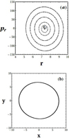Fig. 1. (a) Stroboscopic Poincaré section (r, pr) for f = 2κπ and rc = 7.0, Mb = 6.25 × 1010 M⊙, Ωb = 45 km s−1 kpc−1, and Ωsp = 15 km s−1 kpc−1. (b) The stable periodic orbit of the x1 family.

The orbit derived corresponds to the x₁ family and has an approximately elliptic shape (Fig. 1b). We repeat this procedure for all the radii r_c between 4.4 kpc and 10 kpc with a length step dr = 0.2 kpc, and superimpose the elliptical orbits in Fig. 2a. We observe that these precessing ellipses form a spiral density wave located between their apocenters and pericenters.

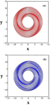Fig. 2. (a) The spiral density wave derived from the periodic orbits of the x1 family for the normal form Hamiltonian (29) of first order $H_{\mathrm{norm}}^{(1)}$ and (b) of second order $H_{\mathrm{norm}}^{(2)}$, for Mb = 6.25 × 1010 M⊙ (a strong bar), Ωb = 45 km s−1 kpc−1, and Ωsp = 15 km s−1 kpc−1.

If we repeat the procedure described above for the second-order normal form $H_{\mathrm{norm}}^{(2)}$ of Eq. (29), we derive a similar spiral density wave with almost no differences from the one derived from the first-order normal form (see Fig. 2b). In fact, the orbits corresponding to the same radius r_c derived by the first- and the second-order normal forms almost coincide, except for a small range of radii around r_c = 9.4 kpc and up to r_c = 9.6 kpc, where there is a small deviation between them. We see that this small deviation results in the appearance of some weak secondary spiral structures, seen as bifurcations from the main spiral, which is something that one can observe in real galaxies. In Fig. 3 we plot a part of the orbits corresponding to the radius r_c = 9.4 kpc derived from the first-order normal form $H_{\mathrm{norm}}^{(1)}$ (in red) and from the second order normal form $H_{\mathrm{norm}}^{(2)}$ (in blue). For this specific radius, we observe the maximum deviation between the two cases.

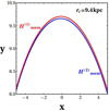Fig. 3. Difference between the periodic orbits of the x1 families derived by the first-order normal form $H_{\mathrm{norm}}^{(1)}$ (red curve) and the second-order normal form $H_{\mathrm{norm}}^{(2)}$ (blue curve) for rc = 9.4 kpc, where the greater deviation between the two orbits occurs.

In general, the spiral density wave derived from the precessing ellipses of the x₁ family, in both cases, is well defined. So, we can now continue with the transformation of the coordinates of the elliptical orbits of the x₁ family to the old variables (r_old, f_old, p_rold, p_fold) (before the normal form construction) using the orbits derived from the first-order normal form Hamiltonian $H_{\mathrm{norm}}^{(1)}$, in order to see how these ellipses are deformed.

3.2. Transformation to the old variables

A back transformation to the old variables (r_old, f_old, p_rold, p_fold) corresponding to the initial, time-dependent Hamiltonian (15), is necessary in order to see how the precessing ellipses forming a well-defined spiral density wave are deformed (from the first- and the second-order normal form constructions) for Ω_b = 45 km s⁻¹ kpc⁻¹ and Ω_sp = 15 km s⁻¹ kpc⁻¹.

We make the back transformation of the spiral density wave derived from the first-order normal form $H_{\mathrm{norm}}^{(1)}$ in the old variables, that correspond to the Hamiltonian (15), which includes the time-dependent angle f₂ = ΔΩt. This transformation is made using the generating function χ. Using the new variables of each periodic orbit x₁ in polar coordinates, (r_new, f_new, p_rnew, p_fnew), and for a specific radius of the circular orbit r_c, we find the old variables (r_old, f_old, p_rold, p_fold) using the following relations:

$$\begin{array}{cc}& r_{\mathrm{old}}=r_{\mathrm{new}}+\{r_{\mathrm{newp}},\chi \}\mathrm{with}{r}_{\mathrm{newp}}=r_{\mathrm{c}}+\sqrt{2J_{\mathrm{r}}/{\kappa }_{\mathrm{c}}}sin{f}_{r_{\mathrm{new}}},\hfill \\ \hfill & f_{\mathrm{old}}=f_{\mathrm{new}}+\{f_{\mathrm{newp}},\chi \}\mathrm{with}{f}_{\mathrm{newp}}=f_{\mathrm{new}},\hfill \\ \hfill & p_{r_{\mathrm{old}}}=p_{r_{\mathrm{new}}}+\{p_{r_{\mathrm{newp}}},\chi \}\mathrm{with}{p}_{r_{\mathrm{newp}}}=\sqrt{2J_{\mathrm{r}}{\kappa }_{\mathrm{c}}}cos{f}_{r_{\mathrm{new}}},\hfill \\ \hfill & p_{f_{\mathrm{old}}}=p_{f_{\mathrm{new}}}+\{p_{f_{\mathrm{newp}}},\chi \}\mathrm{with}{p}_{f_{\mathrm{newp}}}=p_{\mathrm{c}}+J_{\mathrm{u}},\hfill \end{array}$$(31)

where χ is the solution of Eq. (23), $p_{\text{c}}=\mathrm{\Omega }(r_{\text{c}})r_{\text{c}}^2$, and { } defines the Poisson bracket. Using Eq. (18), we can replace cos f_rnew,  sin f_rnew, and J_r in the relations in Eq. (31) as follows: $cos{f}_{r_{\mathrm{new}}}=p_{r_{\mathrm{new}}}/\sqrt{2J_{\mathrm{r}}{\kappa }_{\mathrm{c}}}$, $sin{f}_{r_{\mathrm{new}}}=(r_{\mathrm{new}}-r_{\mathrm{c}})/\sqrt{2J_{\mathrm{r}}/{\kappa }_{\mathrm{c}}}$, and $J_{\text{r}}=(1/(2{\kappa }_{\text{c}}))(p_{r_{\text{new}}}^2+{\kappa }_{\text{c}}{(r_{\text{new}}-r_{\text{c}})}^2)$. Using Eq. (31), we find the perturbed precessing ellipse for each radius r_c of the circular orbit, which includes the information of the second pattern speed of the bar Ω_b in cartesian coordinates (x_old = r_old cos(f_old), y_old = r_old sin(f_old)).

Figure 4 shows the perturbed precessing ellipses for the radii of Fig. 2, derived using the relations in Eq. (31). In particular, Fig. 4a consists of orbits integrated for a short time, namely for ten epicyclic periods (t = 10 T_epi), and Fig. 4b consists of orbits integrated for a longer time, namely for 20 epicyclic periods (t = 20 T_epi), where T_epi = 2π/κ_c and κ_c is the epicyclic frequency given by Eq. (19) for each radius r_c.

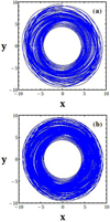Fig. 4. Perturbed precessing ellipses of Fig. 2: (a) for a short integration time corresponding to ten epicyclic periods; and (b) a longer integration time corresponding to 20 epicyclic periods (see text) for Mb = 6.25 × 1010 M⊙ (a strong bar), Ωb = 45 km s−1 kpc−1, and Ωsp = 15 km s−1 kpc−1.

In Fig. 4a it is quite difficult to distinguish the hidden spiral density wave, while in Fig. 4b it is impossible to distinguish any pattern at all. For this reason we used an image processing method in order to recognize the hidden pattern of Figs. 4a,b. The method is described as follows: let G be a grid of L × L square cells (with L = 300) that covers the dimensions of the galactic model (i.e., −12 ≤ x ≤ 12 kpc and −12 ≤ y ≤ 12 kpc). If S = [x(t_i),y(t_i)] is a time series of a single star trajectory on the configuration space, with t_i = iΔt, i = 0, 1, 2, …, I, collected with a time step Δt = 10⁻⁴ (2π/κ_c) (where κ_c is the epicyclic frequency of each orbit given by Eq. (19)) and t = t_I is the total time of the integration of the orbit, then we define the “single star trajectory distribution” P_s(x_j, y_k; t_i) over G around the points (x_j, y_k) = (jΔx, kΔ_y) with j, k = −N, −N + 1, …, N − 1, N, where N = |x_max/Δx|=|y_max/Δy| and x_max = y_max = 12 kpc, as:

$$\begin{array}{c}\hfill P_{\mathrm{S}}(x_j,y_k;t_i)=C_{\mathrm{S}}(x_j,y_k;t_i),\end{array}$$(32)

where C_S is the number of points of the sample S inside the square cell defined by x_j − Δx/2 ≤ x < x_j + Δx/2,  y_k − Δy/2 ≤ y < y_k + Δy/2. Therefore, C_s(x_j, y_k; t_i) is the “single star trajectory occupation number” of the cell (x_j, y_k) from t = 0 up to t = t_I.

The above considerations are easily extended in the case of an ensemble of M trajectories evolved up to t = t_I.

In Fig. 5 we see the result of the processing of Fig. 4b with the method described above. The hidden spiral structure is revealed to be well defined and intense, but slightly deformed in relation to the one of Fig. 2.

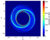Fig. 5. Processed image of Fig. 2b using the method described in the text. A well-defined and intense spiral density wave is presented.

4. Parametric study

The shape of the hidden density wave and how well the spiral structure is maintained in a galactic model containing two different pattern speeds, depend on several parameters, such as the mass of the bar M_b in Eq. (10) and the pattern speed of the bar Ω_b. The perturbation of the precessing ellipses of Fig. 2 depends on the generating function given by Eq. (26). While the mass of the bar M_b affects the coefficients a_{m1, m2, m3} of Eq. (26), the pattern speed of the bar Ω_b is found in the denominator of Eq. (26) in the term ΔΩ = Ω_sp − Ω_b. Therefore, the perturbation of the precessing ellipses becomes greater for greater values of M_b and for smaller absolute values of ΔΩ = Ω_sp − Ω_b, in other words smaller values of Ω_b.

We now make a parametric study for different values of M_b and ΔΩ in order to test the limits inside which the spiral density wave is still detectable.

4.1. The role of the mass of the bar

In order to test the effect of the mass of the bar, we use two smaller values of the value M_b, namely M_b = 3 × 10¹⁰ M_⊙ and M_b = 1 × 10¹⁰ M_⊙, and repeat the procedure described above.

We plot the processed images of the spiral density waves, derived after the transformation to the old variables, for the values of the mass of the bar M_b = 3 × 10¹⁰ M_⊙ in Fig. 6a and M_b = 1 × 10¹⁰ M_⊙ in Fig. 6b. The main observation is that the smaller the mass of the bar, the less intense the spiral density wave of the spiral arms, something that was expected since the coefficients a_{m1, m2, m3}(J_r) of the generating function χ in Eq. (26) depend on the mass M_b of the bar. However, one important remark is that the spirals are well defined and present no breaks, as in the case of the Fig. 5, with the greater value of the bar’s mass M_b. It is now obvious that for even smaller values than M_b = 1 × 10¹⁰ M_⊙, the spiral density wave will gradually disappear.

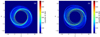Fig. 6. Processed image of the spiral density wave for: (a) Mb = 3 × 1010 M⊙, and (b) Mb = 1 × 1010 M⊙. In both cases Ωb = 45 km s−1 kpc−1 and Ωsp = 15 km s−1 kpc−1.

4.2. The role of the pattern speed of the bar

In order to investigate the role of the pattern speed in the normal form construction of the time-dependent Hamiltonian (15), we repeat the study of the previous subsection but for different values of the pattern speed of the bar Ω_b. We now want to test a slower bar, namely Ω_b = 20 km s⁻¹ kpc⁻¹, and a faster one, namely Ω_b = 60, keeping the bar’s mass constant to M_b = 6.25 × 10¹⁰ M_⊙ as in Fig. 5. Observing in more detail Eq. (26) of the generating function χ, through which the transformation of the normal form is made, we see that the denominator includes the three basic frequencies, namely ΔΩ = Ω_sp − Ω_b, κ_c, and Ω(r_c)−Ω_sp. If we reduce the absolute value of ΔΩ = Ω_sp − Ω_b by using a smaller value of the pattern speed of the bar Ω_b, the perturbation in the normal form construction is greater (a greater value of the generating function χ) and this is reflected in the orbits having a greater deviation from the elliptical form.

We construct the first-order normal form $H_{\mathrm{norm}}^{(1)}$ of Eq. (29) for Ω_b = 20 km s⁻¹ kpc⁻¹ (much slower bar rotation) and for Ω_b = 60 km s⁻¹ kpc⁻¹ (faster bar rotation), and then we repeat the procedure described in Sect. 3.2 in order to reveal the hidden structure of the superposition of the deformed precessing ellipses corresponding to the x₁ periodic families. The spiral density waves derived are shown in Fig. 7. Figure 7a corresponds to Ω_b = 20 km s⁻¹ kpc⁻¹, while Fig. 7b correpsonds to Ω_b = 60 km s⁻¹ kpc⁻¹. We observe that for the case of the slower bar (Ω_b = 20 km s⁻¹ kpc⁻¹), the spiral density wave derived is much less intense compared with Fig. 5, and less well defined as the spiral arms seem to be broken at several radii. On the other hand, in Fig. 7b, where the pattern speed of the bar has a much greater value (Ω_b = 60 km s⁻¹ kpc⁻¹), the spiral density wave seems to be more intense but again it is much less well defined than in Fig. 5. So, there are some upper and lower limits in the value of the pattern speed of the bar in order to have an intense and well-defined spiral density wave structure in a galactic model with two different pattern speeds.

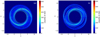Fig. 7. The spiral density wave derived from the periodic orbits of the x1 family for the normal form Hamiltonian (29) of first order, for: (a) a pattern speed of the bar Ωb = 20 km s−1 kpc−1, and (b) a pattern speed of the bar Ωb = 60 km s−1 kpc−1. Both figures have Mb = 6.25 × 1010 M⊙ (a strong bar).

All the calculations were performed on the “superpc” computer with ten CPU cores and 20 threads at the Research Center for Astronomy and Applied Mathematics of the Academy of Athens.

5. Conclusions

In the present paper, we consider a galactic potential of a barred spiral galaxy with two different pattern speeds (for the bar and the spiral arms) and we eliminate the dependence on time of the potential by considering the bar as a perturbation of the spiral potential, in the case where the bar rotates much faster that the spiral arms. The idea is to see how the precessing ellipses that support the spiral structure in the case of a grand design galaxy will be deformed and whether a spiral density wave can still be detected. We use a Milky Way-like model with parameters chosen from Pettitt et al. (2014) and construct a normal form Hamiltonian in first- and second-order approximations, eliminating the time dependence due to the difference between the two pattern speeds.

We find the stable periodic orbits of the x₁ family in this new normal form Hamiltonian and construct the spiral density wave made out of the approximately elliptical orbits of this family. Using the generating function χ, we make a back transformation of these orbits to their original variables where the time is involved. The elliptical periodic orbits are deformed in elliptical rings having a certain thickness. However, if we superimpose all the orbits corresponding to several radii, and using an image processing method, we reveal a slightly deformed spiral density wave that still survives. This result proves that in barred spiral galaxies where the bar rotates much faster that the spiral arms, the spiral structure can be supported by deformed precessing ellipses, such as in the case of grand design galaxies.

We make a parametric study for the values of the bar’s mass and pattern speed. By reducing the bar’s mass, we find less intense but better defined spiral arms. A lower limit of the bar’s mass is approximately the value M_b = 1 × 10¹⁰ M_⊙. By reducing the bar’s pattern speed, we again find less intense spiral density waves and breaks in the spiral arms. Breaks in the spiral density wave appear also in the case of an extremely fast rotating bar (compared with the pattern speed of the spiral arms). The best, well-defined and intense, spiral density wave appears for a ratio of pattern speeds 3 : 1 and a strong bar (M_b = 6.25 × 10¹⁰ M_⊙).

In the case where Ω_b = Ω_sp, the bar can no longer be considered as a perturbation of the spiral potential. This case has been already studied in the framework of the “manifold theory” in a series of papers, as mentioned in the introduction. According to this theory, in the case of barred spiral galaxies with one pattern speed, chaotic orbits with initial conditions along the unstable asymptotic manifolds, emanating from the Lagrandian points L₁ and L₂, as well as nearby sticky chaotic orbits, can support the spiral structures for a long time.

This study is an alternative scenario to the manifold theory, where the spiral potential is considered as a perturbation of the bar potential (see Efthymiopoulos et al. 2020) in the case of a barred spiral galactic model having two different pattern speeds. Here, in contrast, we consider the bar potential as a perturbation of the spiral potential in the case where the bar rotates fast enough, compared with the pattern speed of the spiral arms. This is a proposed scenario for cases of barred spiral galaxies where the spiral arms have a well-defined symmetric shape, such as the one proposed for the Milky Way. In Gerhard (2011), which is a review of the pattern speeds of the Milky Way, the author concludes that the bar of the Milky way is a fast rotator having between double and triple the speed of the spiral arms. In our study we adopt values for the pattern speeds of the bar and the spiral arms that are suggested in Gerhard’s review paper. In the cases where the bar rotates much faster than the spiral arms, as in the case of the Milky Way, the arms in general seem more symmetrical and well defined, having almost the same pitch angle along the entire radius of the galaxy (see also Font et al. 2019 where they give the pattern speeds of the bar and the spiral arms of a fairly large sample of barred spiral galaxies). This image of spiral arms can be supported by ordered elliptical orbits. This is a scenario that is consistent with the density wave theory. Font et al. (2019) also found that the longer the bars (and as a consequence slower), the smallest the differences between the pattern speeds. Thus, the spiral arms, which are most likely bar driven, seem less symmetric with variable pitch angle, while some other features appear such as gaps, bridges, and bifurcations. This image is more consistent with the scenario of chaotic orbits along unstable manifolds supporting the spiral structures. Further numerical investigation is needed in order to confirm such a statement.

So, in conclusion, for the case where the bar rotates much faster than the spiral arms, we suggest an alternative scenario to the “manifold theory” for supporting the spiral structures of the galaxy, which is, in fact, a generalization of the density wave theory.

References

All Figures

	Fig. 1. (a) Stroboscopic Poincaré section (r, pr) for f = 2κπ and rc = 7.0, Mb = 6.25 × 1010 M⊙, Ωb = 45 km s−1 kpc−1, and Ωsp = 15 km s−1 kpc−1. (b) The stable periodic orbit of the x1 family.
In the text

	Fig. 2. (a) The spiral density wave derived from the periodic orbits of the x1 family for the normal form Hamiltonian (29) of first order $H_{\mathrm{norm}}^{(1)}$ and (b) of second order $H_{\mathrm{norm}}^{(2)}$, for Mb = 6.25 × 1010 M⊙ (a strong bar), Ωb = 45 km s−1 kpc−1, and Ωsp = 15 km s−1 kpc−1.
In the text

	Fig. 3. Difference between the periodic orbits of the x1 families derived by the first-order normal form $H_{\mathrm{norm}}^{(1)}$ (red curve) and the second-order normal form $H_{\mathrm{norm}}^{(2)}$ (blue curve) for rc = 9.4 kpc, where the greater deviation between the two orbits occurs.
In the text

	Fig. 4. Perturbed precessing ellipses of Fig. 2: (a) for a short integration time corresponding to ten epicyclic periods; and (b) a longer integration time corresponding to 20 epicyclic periods (see text) for Mb = 6.25 × 1010 M⊙ (a strong bar), Ωb = 45 km s−1 kpc−1, and Ωsp = 15 km s−1 kpc−1.
In the text

	Fig. 5. Processed image of Fig. 2b using the method described in the text. A well-defined and intense spiral density wave is presented.
In the text

	Fig. 6. Processed image of the spiral density wave for: (a) Mb = 3 × 1010 M⊙, and (b) Mb = 1 × 1010 M⊙. In both cases Ωb = 45 km s−1 kpc−1 and Ωsp = 15 km s−1 kpc−1.
In the text

	Fig. 7. The spiral density wave derived from the periodic orbits of the x1 family for the normal form Hamiltonian (29) of first order, for: (a) a pattern speed of the bar Ωb = 20 km s−1 kpc−1, and (b) a pattern speed of the bar Ωb = 60 km s−1 kpc−1. Both figures have Mb = 6.25 × 1010 M⊙ (a strong bar).
In the text

References

- Athanassoula, E. 2012, MNRAS, 426, L46 [NASA ADS] [Google Scholar]
- Athanassoula, E., Romero-Gómez, M., & Masdemont, J. J. 2009a, MNRAS, 394, 67 [NASA ADS] [CrossRef] [Google Scholar]
- Athanassoula, E., Romero-Gómez, M., Bosma, A., & Masdemont, J. J. 2009b, MNRAS, 400, 1706 [NASA ADS] [CrossRef] [Google Scholar]
- Berman, R. H., & Mark, J. W. K. 1977, ApJ, 216, 257 [NASA ADS] [CrossRef] [Google Scholar]
- Boonyasait, V., Patsis, P. A., & Gottesman, S. T. 2005, NYASA, 1045, 203 [NASA ADS] [Google Scholar]
- Buta, R., Vasylyev, S., Salo, H., & Laurikainen, E. 2005, AJ, 130, 506 [NASA ADS] [CrossRef] [Google Scholar]
- Buta, R. J., Knapen, J. H., Elmegreen, B. G., et al. 2009, AJ, 137, 4487 [NASA ADS] [CrossRef] [Google Scholar]
- Cao, L., Mao, S., Nataf, D., Rattenbury, N. J., & Gould, A. 2013, MNRAS, 434, 595 [NASA ADS] [CrossRef] [Google Scholar]
- Contopoulos, G. 1970, Proceedings of IAU. Symposium No 38 (Dordrecht: D. Reidel Publishing Co) [Google Scholar]
- Contopoulos, G. 1971, ApJ, 163, 181 [NASA ADS] [CrossRef] [Google Scholar]
- Contopoulos, G. 1975, ApJ, 201, 566 [NASA ADS] [CrossRef] [Google Scholar]
- Contopoulos, G., & Grosbøl, P. 1986, A&A, 155, 11 [NASA ADS] [Google Scholar]
- Cox, D. P., & Gomez, G. C. 2002, ApJS, 142, 261 [NASA ADS] [CrossRef] [Google Scholar]
- Danby, J. M. A. 1965, AJ, 70, 501 [NASA ADS] [CrossRef] [Google Scholar]
- Dehnen, W. 1993, MNRAS, 265, 250 [NASA ADS] [CrossRef] [Google Scholar]
- Durbala, A., Buta, R., Sulentic, J. W., & Verdes-Montenegro, L. 2009, MNRAS, 397, 1756 [NASA ADS] [CrossRef] [Google Scholar]
- Efthymiopoulos, C. 2012, in Third La Plata Internat. School on Astron. Geophys., eds. P. M. Cincotta, C. M. Giordano, & C. Efthymiopoulos (La Plata: Asociación Argentina de Astronomía) [Google Scholar]
- Efthymiopoulos, C., Harsoula, M., & Contopoulos, G. 2020, A&A, 636, A44 [NASA ADS] [CrossRef] [EDP Sciences] [Google Scholar]
- Font, J., Beckman, J. E., Querejeta, M., et al. 2014, ApJS, 210, 2 [Google Scholar]
- Font, J., Beckman, J. E., James, P. A., & Patsis, P. A. 2019, MNRAS, 482, 5362 [NASA ADS] [CrossRef] [Google Scholar]
- Gerhard, O. 2002, in The Dynamics, Structure and History of Galaxies: A Workshop in Honour of Professor Ken Freeman, eds. G. S. Da Costa, E. M. Sadler, & H. Jerjen, ASP Conf. Ser., 73 [Google Scholar]
- Gerhard, O. 2011, Mem. Soc. Astron. It. Sup., 18, 185 [Google Scholar]
- Grosbøl, P., Patsis, P. A., & Pompei, E. 2004, A&A, 423, 849 [NASA ADS] [CrossRef] [EDP Sciences] [Google Scholar]
- Harsoula, M., Efthymiopoulos, C., & Contopoulos, G. 2016, MNRAS, 459, 3419 [NASA ADS] [CrossRef] [Google Scholar]
- Harsoula, M., Zouloumi, K., Efthymiopoulos, C., & Contopoulos, G. 2021, A&A, 655, A55 [NASA ADS] [CrossRef] [EDP Sciences] [Google Scholar]
- Lin, C., & Shu, F. 1964, ApJ, 140, 646 [Google Scholar]
- Lin, C., & Shu, F. 1966, Proc. Natl. Acad. Sci., 55, 229 [NASA ADS] [CrossRef] [Google Scholar]
- Lindblad, B. 1940, ApJ, 92, 1 [NASA ADS] [CrossRef] [Google Scholar]
- Lindblad, B. 1955, Stockholm Obs. Ann., 18, 6 [Google Scholar]
- Lindblad, B. 1961, Stockholm Obs. Ann., 21, 8 [NASA ADS] [Google Scholar]
- Long, K., & Murali, C. 1992, ApJ, 397, L44 [NASA ADS] [CrossRef] [Google Scholar]
- Meidt, S. E., Rand, R. J., & Merrifield, M. R. 2009, ApJ, 702, 277 [Google Scholar]
- Miyamoto, M., & Nagai, R. 1975, Publ. Astron. Soc. Japan, 27, 533 [Google Scholar]
- Monet, D. G., & Vandervoort, P. O. 1978, ApJ, 221, 87 [NASA ADS] [CrossRef] [Google Scholar]
- Moore, E. M., & Gottesman, S. T. 1995, ApJ, 447, 159 [NASA ADS] [CrossRef] [Google Scholar]
- Patsis, P. A., Contopoulos, G., & Grosbøl, P. 1991, A&A, 243, 373 [NASA ADS] [Google Scholar]
- Pettitt, A. R., Dobbs, C. L., Acreman, D. M., & Price, D. J. 2014, MNRAS, 444, 919 [NASA ADS] [CrossRef] [Google Scholar]
- Quillen, A. C. 2003, ApJ, 125, 785 [CrossRef] [Google Scholar]
- Quillen, A. C., Dougherty, J., Bagley, M. B., Minchev, I., & Comparetta, J. 2011, MNRAS, 417, 762 [NASA ADS] [CrossRef] [Google Scholar]
- Rattenbury, N. J., Mao, S., Sumi, T., & Smith, M. C. 2007, MNRAS, 378, 1064 [NASA ADS] [CrossRef] [Google Scholar]
- Rautiainen, P., & Salo, H. 1999, A&A, 348, 737 [NASA ADS] [Google Scholar]
- Roca-Fàbrega, S., Valenzuela, O., Figueras, F., et al. 2013, MNRAS, 432, 2878 [Google Scholar]
- Romero-Gomez, M., Masdemont, J. J., Athanassoula, E., & Garcia-Gomez, C. 2006, A&A, 453, 39 [NASA ADS] [CrossRef] [EDP Sciences] [Google Scholar]
- Romero-Gomez, M., Athanassoula, E., Masdemont, J. J., & Garcia-Gomez, C. 2007, A&A, 472, 63 [NASA ADS] [CrossRef] [EDP Sciences] [Google Scholar]
- Sarkar, S., & Jog, C. J. 2018, A&A, 617, A142 [NASA ADS] [CrossRef] [EDP Sciences] [Google Scholar]
- Speights, J. C., & Westpfahl, D. J. 2012, ApJ, 752, 52 [NASA ADS] [CrossRef] [Google Scholar]
- Sellwood, J. A., & Sparke, L. S. 1988, MNRAS, 231, 25 [Google Scholar]
- Speights, J. C., & Rooke, P. 2016, ApJ, 826, 2 [NASA ADS] [CrossRef] [Google Scholar]
- Tsoutsis, P., Efthymiopoulos, C., & Voglis, N. 2008, MNRAS, 387, 1264 [NASA ADS] [CrossRef] [Google Scholar]
- Tsoutsis, P., Kalapotharakos, C., Efthymiopoulos, C., & Contopoulos, G. 2009, A&A, 495, 743 [NASA ADS] [CrossRef] [EDP Sciences] [Google Scholar]
- Voglis, N., Tsoutsis, P., & Efthymiopoulos, C. 2006, MNRAS, 373, 280 [NASA ADS] [CrossRef] [Google Scholar]