© ESO 2022

1 Introduction

The Yarkovsky–O’Keefe–Radzievskii–Paddack effect, or YORP, is a torque that emerges in small irregularly shaped asteroids due to the light pressure of scattered and re-emitted radiation. This torque changes the rotation rate and obliquity of asteroids (Vokrouhlický et al. 2015). The normal YORP effect, or NYORP, is created by the recoil forces normal to the overall large-scale surface due to the global shape asymmetry of the asteroid (Rubincam 2000). The tangential YORP effect, or TYORP, is a recoil force dragging the asteroid’s surface in the tangential direction due to uneven heat distribution in the small-scale structures on the surface (Golubov & Krugly 2012).

TYORP has already been modeled numerically for boulders of different shapes: Golubov & Krugly (2012) studied TYORP for one-dimensional high walls, Golubov et al. (2014) and Ševeček et al. (2016) conducted parametric investigations of TYORP for spherical boulders, and Ševeček et al. (2015) simulated a boulder of a complex asymmetric shape.

Therefore, to date only TYORP produced by boulders has been simulated. Nevertheless, the surface of asteroids can contain large spaces between boulders covered with fine regolith (Murdoch et al. 2015), and it is important to estimate this regolith’s contribution to TYORP. On the one hand, regolith in general is flatter than boulders, which decreases its TYORP. On the other hand, it can have a thermal parameter closer to unity, which can increase TYORP. Given this, and in general a bigger area covered by regolith than by boulders, it is uncertain whether boulders or regolith contribute more to TYORP.

A very rough estimate of TYORP produced by regolith was conducted by Golubov (2017). An analytic formula based on multiple simplifying assumptions was used, and it was preliminarily estimated that the regolith could create TYORP of approximately the same order of magnitude as the boulders.

This article aims at a more precise evaluation of TYORP produced by the regolith. It goes beyond the order-of-magnitude estimate of Golubov (2017) and toward a more realistic analytic theory of TYORP for a surface having the shape of a sinusoidal wave. We prefer a sinusoidal wave over other geometries considered in literature, for example concave spherical segments, random Gaussians, and fractals (Davidsson et al. 2015; Rozitis & Green 2011), because a sinusoidal wave allows a simpler analytic treatment in terms of the perturbation theory, and because the Fourier series makes it very convenient for further generalizations and allows an approximate description of other geometries in terms of the sinusoidal Fourier harmonics.

We present a theory for a sinusoidal wave in Sect. 2 and derive an approximate analytic expression for TYORP. In Sect. 3 we study the small-scale shape of the surface of (162173) Ryugu, and then estimate its TYORP in Sect. 4. Section 5 discusses the physical implications of the proposed theory, its limits of applicability, and the possible strength of the effect for other asteroids.

2 Analytic Computation of TYORP for a Sinusoidal Surface

2.1 Non-Dimensionalization of the Heat Conduction Equation

In the dimensional variables, the heat conduction equation has the following form:

$$C\rho \frac{\partial T}{\partial t}=\kappa \left(\frac{{\partial }^{2}T}{\partial X^2}+\frac{{\partial }^{2}T}{\partial Y^2}\right).$$(1)

In this equation T is the temperature, t is the time, С is the heat capacity of the subsurface material, ρ is the density of this material, and κ is its thermal conductivity. Here the coordinates X and Y are defined in such a way that the X-axis is pointing eastward along the asteroid surface and the Y-axis is directed into the depth of the asteroid, with Y being equal to zero on the surface. The curvature of the surface is assumed to be small, and thus it is neglected in the notation of the Laplace operator.

The boundary conditions of the heat conduction equation on the asteroid surface has the following form:

$${\kappa \frac{\partial T}{\partial Y}|}_{Y=0}{=ϵ\sigma T^4|}_{Y=0}-\alpha \Phi \left(1-\text{A}\right).$$(2)

Here ϵ is the emissivity of the asteroid, σ is the Stefan-Boltzmann constant, Φ is the solar constant at the asteroid’s orbit, and A is the asteroid’s albedo. The dimensionless insolation α is defined as the flux of the solar radiation on the surface normalized by the solar constant. The first term in the equation is responsible for the heat flow directed from the depth of the asteroid toward its surface. The next term represents the radiated heat corresponding to the Stefan-Boltzmann law. The last term accounts for the absorption of the solar radiation by the surface of the asteroid.

To simplify the calculations, it is convenient to bring these two equations into dimensionless form. The length scale is defined by the thermal wavelength

$$L_{\text{wave}}=\sqrt{\frac{\kappa }{C\rho \omega },}$$(3)

where ω is the angular velocity of the asteroid. The characteristic temperature is the temperature of the subsolar point:

$$T_0=\sqrt[4]{\frac{\left(1-A\right)\Phi }{ϵ\sigma }.}$$(4)

After non-dimensionalization, all the essential material properties are incorporated into the thermal parameter, which is defined as

$$\theta =\frac{{\left(C\rho \kappa \omega \right)}^{1/2}}{{\left(\left(1-A\right)\Phi \right)}^{3/4}{\left(ϵ\sigma \right)}^{1/4}}.$$(5)

We express distances in units of L_wave, temperatures in units of T₀, and time in units of asteroid rotation phase. Therefore, we obtain the following dimensionless variables: ϕ = ωt, τ = T/T₀, x = X/L_wave, and y = Y/L_wave.

In these notations the heat conduction equation acquires the following form:

$$\frac{\partial \tau }{\partial \varphi }=\frac{{\partial }^2\tau }{\partial x^2}+\frac{{\partial }^2\tau }{\partial y^2}.$$(6)

The boundary condition for this equation is

$${\theta \frac{\partial \tau }{\partial y}|}_{y=0}{={\tau }^4|}_{y=0}-\alpha .$$(7)

Before solving this equation, we determine the insolation α that must be substituted into it.

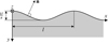Fig. 1 Side view of the asteroid surface. The surface has a sinusoidal shape, with the wavelength l and the amplitude $\frac{kl}{2\pi }$, so that the maximum slope is k. The x-axis is directed along the sine wave, and the у coordinate is measured down from the surface of the asteroid. The normal vector is n.

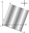Fig. 2 Position of the sine wave on the asteroid surface. The x1- and z1-axes follow the cardinal directions. The x- and z-axes are linked to the sine wave from Fig. 1, and are rotated with respect to the cardinal directions by the azimuthal angle β. The y- and y1-axes are both directed downward and coincide with each other.

2.2 Determination of the Insolation

The geometry of the problem is illustrated in Figs. 1, 2, 3, and 4. The normal to the asteroid surface n and the vector s directed toward the Sun are illustrated in Figs. 1 and 4, which are connected by the coordinate transformations shown in Figs. 2 and 3. In the non-dimensional coordinates, the height of the sinusoidal wave on the surface of regolith (Fig. 1) is given by the equation $\frac{kl}{2\pi }\sin \left(\frac{2\pi x}{l}\right)$, where k is the maximum slope, l = L/L_cond is the dimensionless wavelength, and L is the dimensional wavelength. When determining the orientation of the normal vector, we assume the surface slopes to be small, and thus neglect the terms proportional to k². The azimuthal angle β shows the orientation of the crests of the sine wave with respect to the northward direction on the asteroid surface (Fig. 2). The angle ψ is the latitude of the considered surface element on the asteroid (Fig. 3). The angle ϕ characterizes the position of the Sun with respect to the asteroid (Fig. 4) and is identical to the dimensionless time in Eq. (6). We assume zero obliquity γ = 0, so that the asteroid’s equatorial and orbital planes coincide. In the general case of an arbitrary obliquity, we expect TYORP to be roughly proportional to 1 + cos² γ (Ševeček et al. 2016).

Performing all the coordinate transformations that link Figs. 1 to 4, we obtain the dot product of the surface normal and the unit vector directed toward the Sun,

$$\mathrm{ns}=\cos \varphi \text{cos}\psi -k\sin \left(\frac{2\pi x}{l}\right)\sin \varphi \text{cos}\beta +k\sin \left(\frac{2\pi x}{l}\right)\sin \beta \sin \psi \text{cos}\varphi .$$(8)

The non-dimensional insolation is determined as α = ns H(ns). Here H is the Heaviside step function, which discards the negative values of ns, since the surface is not illuminated by the Sun at night.

We expand this non-linear expression for α into a Fourier series and retain only its first- and second-order terms:

$$\begin{array}{l}\alpha \approx \frac{\cos \psi }{\pi }+\frac{1}{2}\cos \varphi \cos \psi +\frac{k}{\pi }\sin \left(\frac{2\pi x}{l}\right)\sin \psi \sin \beta \hfill \\ -\frac{k}{2}\sin \left(\frac{2\pi x}{l}\right)\sin \varphi \cos \beta +\frac{k}{2}\sin \left(\frac{2\pi x}{l}\right)\sin \beta \sin \psi \cos \varphi .\hfill \end{array}$$(9)

This approximation will decrease the accuracy of our analytic solution, but in most cases it should preserve the correct order of magnitude.

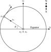Fig. 3 Position of the surface element on the asteroid body. The big circle represents the asteroid; the north pole is at the top, the equator in the middle. The axes x1 and z1 are linked to the surface element from Fig. 2. The latitude ψ is defined as the angle between the equatorial plane and the global normal to the surface −y1. The axes x2, y2, z2 are defined in the asteroid’s body-fixed frame. The axis z2 is aligned with the rotational axis of the asteroid, whereas x2 and y2 are aligned with its equatorial plane and co-rotate with the asteroid.

2.3 Determination of the TYORP Force

When the heat conduction equation is solved and the non-dimensional temperature τ is found, we use it to determine the TYORP force. It is worthwhile to write down the expression for TYORP first, to know beforehand which terms of the temperature we have to retain.

The thermal radiation recoil force acting on the surface area S, which is large with respect to the wavelength L, but small with respect to the asteroid radius, is expressed as

$$F_x{\langle {-\frac{2}{3c}ϵ\sigma T^4|}_{Y=0}{n}_x\cos \beta \rangle }_{X,t}S.$$(10)

The averaging is performed over time t and coordinate X. The factor n_x is the x component of the outer normal to the surface, and c is the speed of light. The coefficient 2/3 arises from averaging the recoil force over Lambert’s emission indicatrix. The minus sign appears because the recoil pressure acts against the surface normal.

It is convenient to express the force F_x in terms of the non-dimensional TYORP pressure p, defining the latter by the equation

$$F_x=\frac{\left(1-A\right)\text{Φ}}{c}pS.$$(11)

Then Eq. (11) is transformed into the following expression for the non-dimensional TYORP pressure:

$$p=-\frac{2}{3}k\cos \beta {\langle {{\tau }^4|}_{y=0}\sin \frac{2\pi x}{l}\rangle }_{x,\varphi }.$$(12)

Now the averaging is performed over the rotation phase φ and the non-dimensional coordinate x. The equation $n_x=k\sin \left(\frac{2\pi x}{l}\right)$ was used for the outer normal to the surface (see Fig. 1).

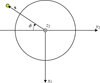Fig. 4 Rotation of the Sun in the asteroid’s body-fixed frame. The big circle represents the north pole view of the asteroid from Fig. 3. The angle ϕ characterizes the time of day on the asteroid. It is measured between the negative y2-axis and the vector s directed toward the Sun.

2.4 Series Decomposition of the Temperature

We now outline the qualitative ideas for our approximate analytic solution of the heat conduction problem, and leave all the algebra for the next subsection. We write the insolation from Eq. (9) in the following form:

$$\alpha ={\alpha }_0+\epsilon {\sin }_x{\sin }_{\varphi }+\epsilon {\sin }_{\varphi }+\epsilon {\sin }_x.$$(13)

Here sin_ϕ denotes a sinusoidal function of ϕ with some unspecified amplitude and phase. Similarly, sin_x is a sinusoidal function of the horizontal coordinate with an unspecified amplitude, phase, wavelength and azimuthal direction. We use the factor ε as a basis to construct a perturbation theory. The temperature will be represented as a series in terms of powers of ε:

$$\tau ={\tau }_0+\epsilon {\tau }_1+{\epsilon }^2{\tau }_2+\dots .$$(14)

We substitute this temperature into Eq. (7), and arrive at the boundary condition in the following form:

$${{\tau }^{\prime }}_0+\epsilon {{\tau }^{\prime }}_1+{\epsilon }^2{{\tau }^{\prime }}_2={\alpha }_0+\epsilon {\sin }_x{\sin }_{\varphi }+\epsilon {\sin }_{\varphi }+\epsilon {\sin }_x-\left({\tau }_0^4+4\epsilon {\tau }_0^3{\tau }_1+4{\epsilon }^2{\tau }_0^3{\tau }_2+6{\epsilon }^2{\tau }_0^2{\tau }_1^2\dots \right).$$(15)

Here we assume that primes denote the y derivatives, and that all the temperatures and their derivatives are calculated at the surface of the asteroid. By equating the coefficients with the identical powers of ε in Eq. (15), the boundary condition can be split into a set of equations:

$$\begin{array}{l}{{\tau }^{\prime }}_0={\alpha }_0-{\tau }_0^4,\hfill \\ {{\tau }^{\prime }}_1={\sin }_x{\sin }_{\varphi }+{\sin }_{\varphi }+{\sin }_x-4{\tau }_0^3{\tau }_1,\hfill \\ {{\tau }^{\prime }}_2=-4{\tau }_0^3{\tau }_2-6{\tau }_0^2{\tau }_1^2.\hfill \end{array}$$(16)

Equation (6) can be similarly decomposed into powers of ε. As a result, we assume that all the terms τ₀, τ₁, τ₂ individually satisfy Eq. (6).

From the first line of Eq. (16), a constant solution for τ₀ can be found. Then from the second line of Eq. (16) and the heat conduction equation Eq. (6), a solution for τ₁ is obtained, which appears to repeat the form of the second line of Eq. (16), τ₁ ~ sin_x sin_ϕ + sin_ϕ + sin_x. The phases and amplitudes of the sin terms are different from those in Eq. (14), but we do not pay attention to them in this qualitative analysis. Next, τ₁ must be squared to be substituted into the third line of Eq. (16), ${\tau }_1^2~{\sin }_x^2{\sin }_{\varphi }^2+{\sin }_x{\sin }_{\varphi }^2+{\sin }_{\varphi }^2+{\sin }_x^2+{\sin }_x^2{\sin }_{\varphi }$. Making use of the addition formulas of trigonometry, we can rewrite it in shorthand notation as ${\tau }_1^2~\left(1+{\sin }_{2x}\right)\left(1+{\sin }_{2\varphi }\right)+{\sin }_x\left(1+{\sin }_{2\varphi }\right)+\left(1+{\sin }_{2\varphi }\right)+\left(1+{\sin }_{2x}\right)+\left(1+{\sin }_{2x}\right){\sin }_{\varphi }$, where the “2” in the lower indexes corresponds to the trigonometric functions of doubled arguments. Finally, opening the brackets and again ignoring the constant multipliers, we get ${\tau }_1^2~1+{\sin }_{\mathrm{2x}}+{\sin }_{\mathrm{2\varphi }}+{\sin }_{\mathrm{2x}}{\sin }_{\mathrm{2\varphi }}+{\sin }_x+{\sin }_{\varphi }+{\sin }_x{\sin }_{\mathrm{2\varphi }}$. This ${\tau }_1^2$ is substituted into the third line of Eq. (16), producing a solution of a similar form: τ₂ ~ 1 + sin_2x + sin_2ϕ + sin_2x sin_2ϕ + sin_x + sin_ϕ + sin_x sin_2ϕ + sin_ϕ sin_2x.

All the components of τ must be substituted into the expression for TYORP pressure $p~{\langle \left({\tau }_0^4+4\epsilon {\tau }_0^3{\tau }_1+4{\epsilon }^2{\tau }_0^3{\tau }_2+6{\epsilon }^2{\tau }_0^2{\tau }_1^2\dots \right){\sin }_x\rangle }_{x,\varphi }.$. Only the terms containing trigonometric functions of neither x nor ϕ survive after averaging. The result is thus produced by the terms sin_x in $4\epsilon {\tau }_0^3{\tau }_1,4{\epsilon }^2{\tau }_0^3{\tau }_2$, and $6{\epsilon }^2{\tau }_0^2{\tau }_1^2$. This finishes the problem of finding the highest-order contribution to p in terms of ε.

The catch is that ε is not small, but is rather on the order of unity. Still, we can expect that the equations that are precise for ε ≪ 1 give a reasonable order-of-magnitude estimate for ε ~ 1, although they are not necessarily precise at any region of the parameter space. This approach is the same as that used by Golubov (2017), which leads to a good agreement between the theory and simulations.

One more thing to be noted from this qualitative analysis is the additivity of waves on the regolith surface. Consider several different sinusoidal spatial waves with non-commensurable wavelengths on the right-hand side of Eq. (13). These terms from Eq. (13) will move to the subsequent equations and mix with each other when expressions get squared or multiplied. Even so, because of the non-commensurability of the wavelengths, the terms independent of the spatial coordinates will arise only from products of terms with the same wavelengths. These are the only ones that create a non-vanishing mean TYORP pressure. It implies that the TYORP pressure is created by each sinusoidal harmonic individually, so that different harmonics with non-commensurable wavelengths do not interfere, and the total TYORP is the sum of TYORPs of different harmonics. Though the case of commensurable wavelengths requires a more sophisticated consideration.

After having outlined the perturbation theory on the qualitative level, we devote the next two subsections to the quantitative realization of the suggested plan.

2.5 Approximate Solution for the Temperature

We solve the heat conduction equation, treating the non-dimensional insolation α in Eq. (9) perturbatively. In the zeroth approximation, we take only the first term in Eq. (9). It is a constant mean insolation, which leads to a constant solution for the non-dimensional temperature: ${\tau }_0=\sqrt[4]{\frac{\cos \psi }{\pi }}.$.

In the next approximation we add the remaining terms in Eq. (9), and find the corrected expression for the temperature, τ = τ₀ + τ₁, which solves the heat conduction in Eq. (6) with the boundary condition in Eq. (7). As τ₀ by itself also solves the heat conduction equation, the same must be true for τ₁ :

$$\frac{\partial {\tau }_1}{\partial \varphi }=\frac{{\partial }^2{\tau }_1}{\partial x^2}+\frac{{\partial }^2{\tau }_1}{\partial y^2}.$$(17)

In the boundary condition in Eq. (7), we assume ${\tau }^4\approx {\tau }_0^4+4{\tau }_0^3{\tau }_1$ and neglect the higher-order terms. The principal term of α cancels ${\tau }_0^4$, and the boundary condition for τ₁ acquires the following form:

$${\theta \frac{\partial {\tau }_1}{\partial y}|}_{y=0}{-4{\tau }_0^3{\tau }_1|}_{y=0}=\frac{1}{2}\cos \psi \cos \varphi -\frac{k}{\pi }\sin \left(\frac{2\pi x}{l}\right)\sin \beta \sin \psi +\frac{k}{2}\sin \left(\frac{2\pi x}{l}\right)\cos \beta \sin \varphi -\frac{k}{2}\sin \left(\frac{2\pi x}{l}\right)\sin \beta \sin \psi \cos \varphi .$$(18)

The solution of this inhomogenous linear problem can be found as the sum of solutions corresponding to individual inhomogeneities on the right-hand side of Eq. (18). Each inhomogeneity has a sinusoidal dependence on ϕ and x, which in terms of complex variables can be treated as an exponential dependence. We allow for an exponential dependence on y as well, and substitute this product of three exponents into Eq. (17). It turns the partial differential equation into a quadratic algebraic equation for the unknown factor standing in front of y in the exponent. We choose only those roots of this quadratic equation that correspond to an exponential decrease in τ₁ at large depths, not an exponential increase. Then the pre-exponential factor is chosen to satisfy Eq. (18). Performing this procedure for each inhomogeneity in Eq. (18), we find the following solution for τ₁ :

$${\tau }_1=e^{-\frac{y}{\sqrt{2}}}\left(a_1\cos \left(\varphi -\frac{y}{\sqrt{2}}\right)+a_2\sin \left(\varphi -\frac{y}{\sqrt{2}}\right)\right)+b_1\exp \left(-\frac{2\pi y}{l}\right)\sin \left(\frac{2\pi x}{l}\right)+e^{-\text{μ}y}\left(c_1\cos \varphi \cos \left(\frac{2\pi x}{l}-vy\right)+c_2\cos \varphi \sin \left(\frac{2\pi x}{l}-vy\right)+c_3\sin \varphi \cos \left(\frac{2\pi x}{l}-vy\right)+c_4\sin \varphi \sin \left(\frac{2\pi x}{l}-vy\right)\right).$$(19)

The coefficients entering this solution are expressed as

$$\begin{array}{l}{a}_1=a_2\left(1+\frac{4\sqrt{2}{\tau }_0^3}{\theta }\right)=\frac{\left(1+\frac{4\sqrt{2}{\tau }_0^3}{\theta }\right)\cos \psi }{\sqrt{2}\theta \left(1+{\left(1+\frac{4\sqrt{2}{\tau }_0^3}{\theta }\right)}^2\right)},\hfill \\ b_1=\frac{k}{\pi \left(4{\tau }_0^3+\frac{2\pi \theta }{l}\right)},\hfill \\ c_1=-c_3\frac{\cos \beta }{\sin \beta \sin \psi }=\frac{\frac{-k}{2\theta v}\sin \beta \sin \psi }{1+{\left(\frac{\text{μ}}{v}+\frac{4{\tau }_0^3}{v\theta }\right)}^2},\hfill \\ c_2=-c_4\frac{\cos \beta }{\sin \beta \sin \psi }=\frac{\frac{k}{2\theta v}\sin \beta \sin \psi \left(\frac{\text{μ}}{v}+\frac{4{\tau }_0^3}{v\theta }\right)}{1+{\left(\frac{\text{μ}}{v}+\frac{4{\tau }_0^3}{v\theta }\right)}^2}.\hfill \end{array}$$(20)

The constants μ and v in these equations are defined as

$$\begin{array}{l}\text{μ}=\frac{1}{\sqrt{2}}{\left(\sqrt{1+{\left(\frac{2\pi }{l}\right)}^4}+{\left(\frac{2\pi }{l}\right)}^2\right)}^{\frac{1}{2}},\hfill \\ v=\frac{1}{\sqrt{2}}{\left(\sqrt{1+{\left(\frac{2\pi }{l}\right)}^4}-{\left(\frac{2\pi }{l}\right)}^2\right)}^{\frac{1}{2}}.\hfill \end{array}$$(21)

Next, we implement the second correction to the temperature: τ = τ₀ + τ₁ + τ₂. In a similar way, we obtain the following equation and the boundary condition for τ₂:

$$\frac{\partial {\tau }_2}{\partial \varphi }=\frac{{\partial }^2{\tau }_2}{\partial x^2}+\frac{{\partial }^2{\tau }_2}{\partial y^2},$$(22)

$${\theta \frac{\partial {\tau }_2}{\partial y}|}_{y=0}-{4{\tau }_0^3{\tau }_2|}_{y=0}={6{\tau }_0^2{\tau }_1^2|}_{y=0}.$$(23)

Solving this equation at full length would be very tedious, and would produce a very cumbersome answer. We show in the next subsection, however, that only one particular term from τ₂ is needed to estimate TYORP.

2.6 Derivation of the TYORP Force from the Approximate Expression for the Temperature

We substitute the approximate expression for the non-dimensional temperature τ = τ₀ + τ₁ + τ₂ into the expression for the TYORP force given by Eq. (12), neglecting the terms that contain high powers of τ₁ and τ₂:

$$p=-\frac{2}{3}k\cos \beta {\langle \left({\tau }_0^4+4{\tau }_0^3{\tau }_1+6{\tau }_0^2{\tau }_1^2+4{\tau }_0^3{\tau }_2\right)\sin \frac{2\pi x}{l}\rangle }_{x,\varphi }.$$(24)

The ${\tau }_0^4$ term gives zero when averaged over x. In all other terms of τ⁴ only those independent of ϕ and proportional to sin $\frac{2\pi x}{l}$ survive after averaging.

The only surviving term in the expression for pressure, which comes from $4{\tau }_0^3{\tau }_1$, is the one proportional to b₁:

$$p_{\beta }=-\frac{k^2\pi {\tau }_0^2{\theta }^3\left(4{\tau }_0^3+\text{μ}\theta \right)\left(4\sqrt{2}{\tau }_0^3+\theta \right)}{2\sqrt{2}\left(2l{\tau }_0^3+\pi \theta \right)\left(16{\tau }_0^6+4\sqrt{2}{\tau }_0^3\theta +{\theta }^2\right)}\times \frac{\cos \psi \sin \psi \cos \beta \sin \beta }{16{\tau }_0^6+8\text{μ}{\tau }_0^3\theta +\left({\text{μ}}^2+v^2\right){\theta }^2}.$$(25)

Its physical meaning is that the southern slopes of the sinusoidal mounds are warmer and radiate more heat to the west or east, depending on the azimuth β. Although this term can be the dominating one for small patches of the surface, we do not expect it to produce any significant TYORP for the asteroid as a whole. The reason is the absence of any asymmetry in the azimuth β between the northeast and northwest orientations of the waves, leading to a near-zero average of Eq. (25) over the asteroid surface. We thus disregard this term in our further consideration.

After squaring Eq. (19), we can see that the only component of $6{\tau }_0^2{\tau }_1^2$ surviving after averaging in Eq. (24) is

$$p_1=-2k\cos \beta {\tau }_0^2\left(a_1{c}_2+a_2{c}_4\right).$$(26)

From the form of the last term in Eq. (24), $4{\tau }_0^3{\tau }_2$, we can conclude, that the only component of τ₂ contributing to TYORP is the one proportional to sin $\frac{2\pi x}{l}$ and independent of ϕ. From Eqs. (22) and (23) we see that these terms in τ₂ are produced by the corresponding terms in ${\tau }_1^2$ that are also proportional to sin $\frac{2\pi x}{l}$ and independent of ϕ. We search for this term in the form of the product of exponents depending on x and y. We substitute the product of the exponents into Eq. (22), and thus find the dependence of the studied term on y. Then we substitute this term into the boundary condition Eq. (23) to find the pre-exponential factor. The resulting expression of the only relevant term in τ₂ is the following:

$${\tau }_2=-\frac{6{\tau }_0^2\left(a_1{c}_2+a_2{c}_4\right)}{\frac{2\pi \theta }{l}+4{\tau }_0^3}\sin \left(\frac{2\pi x}{l}\right)\exp \left(-\frac{2\pi y}{l}\right).$$(27)

Finally, we substitute this expression into Eq. (24), and find the contribution of τ₂ to TYORP:

$$p_2=8k\cos \beta {\tau }_0^3\frac{{\tau }_0^2\left(a_1{c}_2+a_2{c}_4\right)}{\frac{2\pi \theta }{l}+4{\tau }_0^3}.$$(28)

Adding up Eqs. (26) and (28), and substituting the coefficients a₁, a₂, c₂, and c₄ from Eq. (20), we derive the final expression for the non-dimensional TYORP pressure:

$$p=\frac{k^2\pi {\tau }_0^2{\theta }^2\left(4{\tau }_0^3+\text{μ}\theta \right)}{2\sqrt{2}\left(2l{\tau }_0^3+\pi \theta \right)\left(16{\tau }_0^6+4\sqrt{2}{\tau }_0^3\theta +{\theta }^2\right)}\times \frac{\cos \psi {\cos }^2\beta }{16{\tau }_0^6+8\text{μ}{\tau }_0^3\theta +\left({\text{μ}}^2+v^2\right){\theta }^2}.$$(29)

According to this equation, TYORP depends on the following physical parameters: the thermal parameter θ, the non-dimensional wavelength l, the azimuth β, the latitude ψ, and the maximum slope k. The remaining three values μ, v, and τ₀ are expressed in terms of other parameters.

The dependence of p on θ and l as given by Eq. (29) is illustrated in Figs. 5–7. The two panels of Fig. 5 show the dependence on θ and l separately. Figure 6 color-codes p as a function of θ and l simultaneously, so that the lines on the left- and right-hand sides of Fig. 6 correspond to the individual vertical and horizontal cross-sections of Fig. 5, respectively. We see that TYORP is maximum at l ~ θ ~ 1, and rapidly decays at smaller and larger l or θ.

The trends shown in Fig. 5 are similar to that presented in Fig. 8 of Golubov (2017), if l from this article is equated to λ from Golubov (2017), and p/k² from this article is equated to p/α² from Golubov (2017). The maximum p/α² from Golubov (2017) is about 0.012, which is almost 2.5 times larger than the maximum in Figs. 5 and 6.

Figure 7 illustrates the dependence of the total TYORP force p_β + p (Eqs. (25) and (29) combined) on β and θ. Both p_β and p are periodic in β with the period π, but p vanishes at $\beta =\frac{\pi }{2}$ and reaches its maximum at β = 0, whereas p_β vanishes at β = 0 and $\beta =\frac{\pi }{2}$, reaches its maximum at $\beta =\frac{\pi }{4}$ and minimum at $\beta =\frac{3\pi }{4}$. At θ → 0, both p_β and p vanish. At θ → ∞, p vanishes and p_β reaches its maximum. Despite the rich physics and beauty of Fig. 7, it presents mostly an academic interest because p_β vanishes after averaging over β, and thus only p is important for the global TYORP.

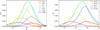Fig. 5 Non-dimensional TYORP pressure determined by Eq. (29) as a function of l and θ. Left panel: dependence on θ for several fixed values of l. Right panel: dependence on l for several fixed values of θ. The other parameters are ψ = 0, β = 0.

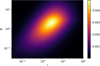Fig. 6 Color map showing the non-dimensional TYORP pressure determined by Eq. (29) as a function of l and θ. The other parameters are ψ = 0, β = 0.

3 Analysis of the Shape of (162173) Ryugu

As a sample of the asteroid surface, we used the cross-section of a region on the asteroid (162173) Ryugu determined by the MASCOT lander of the Hayabusa2 space mission (Scholten et al. 2019; Otto et al. 2021). It is 40 cm in length and has a 3mm spatial resolution.

We want to determine the typical maximum slope k(l) corresponding to each wavelength l, in order to substitute it into Eq. (29). For this, we need a measure of curvature of the surface at each l. As a simple measure of curvature we adopt the following function:

$$\lambda \left(h\right)={\langle {\left(y\left(x+h\right)-2y\left(x+\frac{h}{2}\right)+y\left(x\right)\right)}^2\rangle }_x.$$(30)

This function is proportional to the mean value of the square of the second-order divided difference for the height as a function of the horizontal coordinate x, with h being the distance scale at which the divided difference is computed. If the height y(x) has a constant slope, the second-order divided difference vanishes, and λ(h) = 0. If the surface is sinusoidal with the wavelength l and the maximum slope k (i.e., $y\left(x\right)=\frac{kl}{2\pi }\sin \left(\frac{2\pi x}{l}\right)$ it can be easily shown that

$$\lambda \left(h\right)=2{\left(\frac{kl}{\pi }\right)}^2{\sin }^4\left(\frac{\pi h}{2l}\right).$$(31)

The maximum contribution to λ(h) is produced by waves with wavelengths l such that $\frac{\pi h}{2l}=\frac{\pi }{2}+\pi n$, where n ∈ ℕ₀, that is l = h/(2n + 1). As the terms of this series decay rapidly with n, we approximate the entire series by its first term. Thus, we equate the experimentally determined λ(l) from Eq. (30) to the theoretical λ(l) from Eq. (31) for the same wavelength l. This results in the following expression for the maximum slope of a sinusoidal wave of a given wavelength:

$$k\left(l\right)=\frac{\pi }{l}\sqrt{\frac{\lambda \left(l\right)}{2}}.$$(32)

We apply this equation to the cross-section of Ryugu from Fig. 2c in Otto et al. (2021). The resulting slope k(l) as a function of the wavelength is shown in Fig. 8. The plot shows the entire range from 3 mm (the spatial resolution of the original cross-section) to 40 cm (the total length of the studied cross-section). Close to these limits the measured k(l) has a lower accuracy: due to the loss of small-scale features when l is close to the spatial resolution, and due to the insufficient statistics when l is close to the maximum length. We show these less certain regions with dashed lines in Fig. 8.

This slope k must be substituted into Eq. (29) to get the TYORP pressure for the asteroid. We note that here we assumed that the waves have zero azimuth, β = 0. For a different azimuth the factor cosβ will appear in the denominator of the right-hand side of Eq. (32), but it will be canceled by the cosβ in the numerator of Eq. (29). Another cosβ will appear in the argument of the left-hand side of Eq. (32), but this horizontal stretching of Fig. 8 will leave the near-horizontal part of the plot at the same level and will not effect the resulting TYORP. Thus, we just ignore the factors cosβ everywhere in our estimate and assume β = 0.

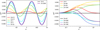Fig. 7 Illustration of the dependence of the non-dimensional TYORP pressure determined by Eq. (29) on the azimuthal angle β. Left panel: dependence on β for several fixed values of θ. Right panel: dependence on θ for several fixed values of β. The other parameters are l = 1, ψ = 0.

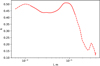Fig. 8 Effective slope of sinusoidal waves of different wavelengths, computed via Eq. (32) for the shape of asteroid (162173) Ryugu presented in Otto et al. (2021).

4 Results

The TYORP pressure must be integrated over the surface of the asteroid. We assume the asteroid to be spherical, and to have a zero obliquity and a circular orbit. In the dimensional units, the resulting TYORP torque is

$$T_{\omega }=\frac{\left(1-A\right)\Phi R^3}{c}{p}_{0}2\pi {\displaystyle {\int }_{-\frac{\pi }{2}}^{\frac{\pi }{2}}{\cos }^3\psi \text{d}\psi }.$$(33)

The lower index ω marks the component of the torque that changes the rotation rate ω of the asteroid. In this equation R is the radius of the asteroid, and p₀ is the value of Eq. (29) at ψ = 0. The third power of cos ψ originates because one term cos ψ comes from Eq. (29), one from the surface element 2πR² cos ψdψ, and one from the lever arm R cos ψ.

Introducing the non-dimensional TYORP torque ${\tau }_{\omega }=\frac{c}{\Phi R^3}{T}_{\omega }$ and performing integration in Eq. (33), we arrive at the following final expression for TYORP of the asteroid:

$$T_{\omega }=\left(1-A\right)p_0\frac{8\pi }{3}.$$(34)

We apply this formula to estimate TYORP of asteroid Ryugu. We assume the rotation period 7.63 h, the albedo A = 0.045 (Watanabe et al. 2019), the thermal emissivity ∊ = 0.9 (Hamm 2019), the density of the subsurface material equal to the mean asteroid density ρ = 1190 kg m⁻³ (Watanabe et al. 2019), the thermal inertia $\Gamma =\sqrt{\kappa C\rho }=225$ J m⁻² K⁻¹ (Shimaki et al. 2020), and the heat capacity к = 700 J kg⁻¹ K⁻¹, which is typical for chondrite material (Szurgot 2011). Substituting these values into Eqs. (3) and (5), we get the thermal parameter θ = 1.34 and the thermal wavelength L_wave =1.8 cm.

For this thermal parameter, the maximum TYORP pressure is p ≈ 0.0048k², and the maximum is attained at the non-dimensional wavelength l ≈ 4 (see Fig. 5). It corresponds to the dimensional wavelength L = L_wavel ≈ 7 cm. The slope at this wavelength is k ≈ 0.5 (see Fig. 8). It results into the maximum non-dimensional TYORP pressure p₀ ≈ 0.0012. Substituting this value into Eq. (34), we obtain the non-dimensional TYORP produced by the surface roughness on Ryugu equal to τ≈ 0.01.

Kanamaru et al. (2021) uses the shape model of Ryugu revealed by Hayabusa2 to compute the normal YORP. The resulting acceleration is negative and lies in the range −0.42 × 10⁻⁶ deg day⁻² to −6.3 × 10⁻⁶ deg day⁻². Such a large discrepancy between different shape models even at a very high resolution is not surprising. Extreme sensitivity of YORP to fine details of the shape models have been theoretically investigated by Statler (2009). Similar YORP differences for shape models of different (but very high) resolution have also been observed in simulations of asteroid Itokawa (Scheeres et al. 2007). Ryugu’s accelerations obtained by Kanamaru et al. (2021) correspond to the non-dimensional torque τ_ω of the normal YORP in the range from −0.00014 to −0.0021. The tangential YORP τ_ω ≈ 0.01 derived from our model can surpass this value, causing a positive net acceleration despite the negative YORP produced by the asteroid shape asymmetry.

5 Discussion

In this paper we constructed the theory of TYORP of a rough surface in application to the asteroid’s regolith, but the same theory is applicable for the surface roughness of boulders, which can be described by the same equations but with different thermal parameters. Such surface roughness adds up to the torque created by the smooth boulders and can enhance TYORP. The largest TYORP is produced by the shape irregularities at the spatial scale on the order of L_wave, which can correspond to small boulders as a whole, and to surface roughness on large boulders. For a typical largely cracked protrusion it can be impossible to tell whether it is an individual boulder or a bump on the surface of a larger boulder. This makes a smooth transition between TYORP produced by boulders and by surface roughness. To some degree of accuracy it can even be possible to express TYORP of gently sloped boulders in terms of this article by Fourier-decomposing the boulder shapes.

For the typical asteroid thermal inertias Г ~ 10−700 J m⁻² s⁻⁰⁵ K⁻¹ (Hanuš et al. 2018), densities ρ ~ 1000−5000 kg m⁻³, rotation periods P_rot ~ 2−30 h, and orbital semi-major axes a ~ 1−3 AU, we obtain the thermal parameters θ ~ 0.01−10 and thermal wavelengths L_wave ~ 10⁻⁴−10⁻¹ m. The resulting thermal parameters are close to the values that produce the maximum TYORP (see Fig. 5). The thermal wavelengths give us the scale at which the roughness produces the largest contribution to TYORP. Unfortunately, the information about the roughness of asteroids at such a short scale is very limited. Moreover, it is questionable whether at submillimeter scale the asteroid material can be considered a continuous medium, thus violating the underlying assumptions of our model.

If the rough surface elements have high tilts with respect to the horizon, they are shadowed more often than Eq. (8) assumes, which diminishes the TYORP produced by them. Other intrinsic limitations of the proposed theory include the possible non-uniformity of the granular material at the Lwave scale, as well as the possible non-constancy of к as a function of temperature if a large fraction of energy is transferred by radiation (see e.g. Ryan et al. 2020). These effects could be incorporated in the theory at a later stage. Most importantly, the suggested analytic theory needs to be verified by numeric simulations, but we will deal with this part in the subsequent paper.

Acknowledgements

This work was supported by the National Research Foundation of Ukraine, project N2020.02/0371 “Metallic asteroids: search for parent bodies of iron meteorites, sources of extraterrestrial resources". We are grateful to Ukrainians who are fighting to stop the war so that we can safely finish the revision of this article. We are also grateful to our reviewer Masanori Kanamaru for comments that helped to improve the article.

References

All Figures

	Fig. 1 Side view of the asteroid surface. The surface has a sinusoidal shape, with the wavelength l and the amplitude $\frac{kl}{2\pi }$, so that the maximum slope is k. The x-axis is directed along the sine wave, and the у coordinate is measured down from the surface of the asteroid. The normal vector is n.
In the text

	Fig. 2 Position of the sine wave on the asteroid surface. The x1- and z1-axes follow the cardinal directions. The x- and z-axes are linked to the sine wave from Fig. 1, and are rotated with respect to the cardinal directions by the azimuthal angle β. The y- and y1-axes are both directed downward and coincide with each other.
In the text

Fig. 3 Position of the surface element on the asteroid body. The big circle represents the asteroid; the north pole is at the top, the equator in the middle. The axes x1 and z1 are linked to the surface element from Fig. 2. The latitude ψ is defined as the angle between the equatorial plane and the global normal to the surface −y1. The axes x2, y2, z2 are defined in the asteroid’s body-fixed frame. The axis z2 is aligned with the rotational axis of the asteroid, whereas x2 and y2 are aligned with its equatorial plane and co-rotate with the asteroid.

In the text

	Fig. 4 Rotation of the Sun in the asteroid’s body-fixed frame. The big circle represents the north pole view of the asteroid from Fig. 3. The angle ϕ characterizes the time of day on the asteroid. It is measured between the negative y2-axis and the vector s directed toward the Sun.
In the text

	Fig. 5 Non-dimensional TYORP pressure determined by Eq. (29) as a function of l and θ. Left panel: dependence on θ for several fixed values of l. Right panel: dependence on l for several fixed values of θ. The other parameters are ψ = 0, β = 0.
In the text

	Fig. 6 Color map showing the non-dimensional TYORP pressure determined by Eq. (29) as a function of l and θ. The other parameters are ψ = 0, β = 0.
In the text

	Fig. 7 Illustration of the dependence of the non-dimensional TYORP pressure determined by Eq. (29) on the azimuthal angle β. Left panel: dependence on β for several fixed values of θ. Right panel: dependence on θ for several fixed values of β. The other parameters are l = 1, ψ = 0.
In the text

	Fig. 8 Effective slope of sinusoidal waves of different wavelengths, computed via Eq. (32) for the shape of asteroid (162173) Ryugu presented in Otto et al. (2021).
In the text

References

- Davidsson, B. J., Rickman, H., Bandfield, J. L., et al. 2015, Icarus, 252, 1 [CrossRef] [Google Scholar]
- Golubov, O. 2017, AJ, 154, 238 [NASA ADS] [CrossRef] [Google Scholar]
- Golubov, O., & Krugly, Y. N. 2012, ApJ, 752, L11 [NASA ADS] [CrossRef] [Google Scholar]
- Golubov, O., Scheeres, D. J., & Krugly, Y. N. 2014, ApJ, 794, 22 [NASA ADS] [CrossRef] [Google Scholar]
- Golubov, O., Kravets, Y., Krugly, Y. N., & Scheeres, D. J. 2016, MNRAS, 458, 3977 [NASA ADS] [CrossRef] [Google Scholar]
- Hamm, M. 2019, PhD Thesis, Freie Universitat Berlin, Germany [Google Scholar]
- Hanuš, J., Delbo, M., Ďurech, J., & Ali-Lagoa, V. 2018, Icarus, 309, 297 [CrossRef] [Google Scholar]
- Kanamaru, M., Sasaki, S., Morota, T., et al. 2021, J. Geophys. Res. Planets, 126, e2021JE006863 [CrossRef] [Google Scholar]
- Murdoch N., Sánchez P., Schwartz S. R., & Miyamoto, H. 2015, in Asteroids IV, eds. P. Michel, F. E. DeMeo, & W. F. Bottke, (Tucson: University of Arizona), 767 [Google Scholar]
- Otto, K. A., Matz, K. D., Schröder, S. E., et al. 2021, MNRAS, 500, 3178 [Google Scholar]
- Rozitis, B., & Green, S. F. 2011, MNRAS, 415, 2042 [NASA ADS] [CrossRef] [Google Scholar]
- Rubincam, D. P. 2000 Icarus, 148, 2 [Google Scholar]
- Ryan, A. J., Pino Munoz, D., Bernacki, M., & Delbo, M. 2020, J. Geophys. Res. Planets, 125, e06100 [NASA ADS] [CrossRef] [Google Scholar]
- Scholten, F., Preusker, F., Elgner, S., et al. 2019, A&Amp;A, 632, L5 [NASA ADS] [CrossRef] [EDP Sciences] [Google Scholar]
- Ševeček, P., Brož, M., Čapek, D., & Ďurech, J. 2015, MNRAS, 450, 2104 [CrossRef] [Google Scholar]
- Ševeček, P., Golubov, O., Scheeres, D. J., & Krugly, Y. N. 2016, A&Amp;A, 592, A115 [NASA ADS] [CrossRef] [EDP Sciences] [Google Scholar]
- Scheeres, D. J., Abe, M., Yoshikawa, M., et al. 2007, Icarus, 188, 425 [NASA ADS] [CrossRef] [Google Scholar]
- Shimaki, Y., Senshu, H., Sakatani, N., et al. 2020, Icarus, 348, 113835 [Google Scholar]
- Statler, T. S. 2009, Icarus, 202, 502 [NASA ADS] [CrossRef] [Google Scholar]
- Szurgot, M. 2011, Lunar Planet. Sci. Conf., 1608, 1150 [Google Scholar]
- Vokrouhlický, D., Bottke, W. F., Chesley, S. R., Scheeres, D. J., & Statler, T. S. 2015, in Asteroids IV, eds. P. Michel, F. E. DeMeo, & W. F. Bottke, (Tucson: University of Arizona), 509 [Google Scholar]
- Watanabe, S., Hirabayashi, M., Hirata, N., et al. 2019, Science, 364, 268 [NASA ADS] [Google Scholar]