© X. J. Xi and A. Vienne 2022

1 Introduction

The numerical integration ephemerides of natural satellites are widely used for their high precision. However, this advantage does not promote their use in the scientific studies of rotation and evolution as their finite time spans place serious restrictions on obtaining the motion details from the ephemerides. We work to represent the numerical integration ephemerides in the form of combinations of related proper frequencies, called the analytical representation, which have the advantages of long-lasting stability and high precision. This representation explicitly describes the motion details of the planet system.

In our previous work (Xi & Vienne 2020; hereafter Paper I), we successfully obtained the representation of the mean longitude of the JPL Titan ephemeris (Giorgini et al. 1996). Meanwhile, we obtained the proper frequencies involved using TASS as a template (Vienne & Duriez 1995). The representation included the mean motion, the constant term, and the amplitudes and phases of eight periodic and quasi-periodic terms. The mean residuals between JPL and our representation was about −13.27 m, and the standard deviation was about 26km. Encouraged by these satisfactory results, we extend our study to the other orbital elements of Titan.

As in Paper I, here we take the TASS ephemerides as a template to successfully demonstrate how to obtain the representations of the JPL Titan ephemerides. We work on the analytical representations of the other five orbital elements: the eccentricity and the pericentre $z_6:e_6\cdot e^{\sqrt{-1{\varpi }_6}}$; the inclination and the ascending node ${\zeta }_6:\sin \frac{i_6}{2}\cdot {\text{e}}^{\sqrt{-1{\text{Ω}}_6}}$; and the semi-major axis a₆. The elements z₆ and ζ₆ are complex, hence each corresponds to two elements.

In Sect. 2, we give some important additional information on the JPL ephemerides and the update in early 2020. In Sect. 3, we report the short terms and semi-long terms of ζ₆ and z₆ by frequency analysis. They are later removed to simplify the calculation.

A nominal value of the proper frequency for the ascending node of Titan ${\text{Ω}}_6^{*}$, according to a TASS formula, is adopted from Paper I. This nominal value plays an important role in the analytical representation of ζ₆ in this study. The discussion related to ζ₆ is presented in Sect. 4.

Our experience with ζ₆ promotes us to further analyse the residuals in order to find the additional short-term components. These terms usually have very small amplitudes, one or two orders of magnitude less than the major ones. Thus, they exist but are hidden in the residuals. The representation of z₆ is displayed in Sect. 5.

The representation of the semi-major axis a₆ (Sect. 6), which involves numerous short-period terms, and the updated mean longitude λ₆ (Sect. 7) are conducted in this study. The latter now has 15 instead of 8 components, as well as a smaller standard deviation.

Put together, we can report the representations of all the elliptic elements of Titan (Sect. 8). The representations have almost the same precision as the original Titan ephemeris of JPL with the same time duration. However, the dynamic information that they contain can be used over a much longer time period. All the derived equations used in the study are listed in the Appendix. A more detailed description of the synthetic representation of the motion can be found in Paper I.

2 Ephemerides Information

It is necessary to mention some information on the ephemerides. As was done in Paper I, each orbit of the satellites in this study is described by the osculating elements p, λ, z, and ζ, following the work of Duriez (Duriez 1979, 1977): $$\begin{array}{l}a=A{\left(1+p\right)}^{-2/3}\iff n=N\left(1+p\right),\hfill \\ \lambda =Nt+{\lambda }_0+r,\hfill \\ z=e\exp \sqrt{-1\varpi ,}\hfill \\ \zeta =\sin \frac{i}{2}\exp \sqrt{-1\Omega }.\hfill \end{array}$$(1)

The JPL ephemerides are presented in either the classical elliptic element form as (a, e, i, ω, ϖ, M) or the position-velocity form in the ecliptic plane. The quantity µ in Kepler’s third law n²a³ = µ used in this study is $$\mu =10129767089077\times {10}^{-2}\left({\text{au}}^3{\text{y}}^{-2}\right)$$(2)

Here, au means astronomical units and y is year.

All motions refer to the Saturnicentric ring plane in which the origin corresponds to the node with the mean ecliptic J2000. The node and the inclination refer to the equinox and ecliptic J2000 system and are then defined as $$\begin{array}{c}{\Omega }_{\text{a}}={169.5291}^{\circ },\\ i_a={28.0512}^{\circ }.\end{array}$$(3)

The orbital elements of JPL are transformed into the same form as (a, λ, z, ζ) on the Saturn ring plane with Eqs. (2) and (3).

An update was made by JPL to the ephemerides of its Saturnian satellites in early 2020 based on the final Cassini comprehensive reconstruction. However, the available time span of the new version is about 500 yr, which does meet our computation requirements. In this research we use the same ephemeris of Titan as in Paper I, which was first published in 2016 with an official accuracy of 10 km. The corresponding ephemeris is available upon request. All the physical parameters of the Solar System were downloaded from the JPL official website in 2019.

For simplicity, we abbreviate some of the repeated concepts in this study. We refer to the TASS template as TASS-t (see Paper I), which corresponds to the representations of all the orbital elements of TASS, with all the proper frequencies of the Saturn system. Similarly, XA-JPL represents all the parameters, proper frequencies, and representations of the JPL ephemerides. FA is the abbreviation for frequency analysis, and LSM for the least-squares method.

The proper frequencies related to the representations are the following:

The proper frequencies of TASS and JPL relative to this work can be found in Table 1. The superscript asterisk (*) indicates a corresponding argument to the proper frequencies. Proper frequencies are the physical characteristics, thus their values remain constant throughout the corresponding dynamical system. However, readers can find small differences in their values between Table 1 and the other tables. For example, we see the different values of λ_s in Table 1, Table 7, and Table 11. The value of λ_s in Table 7 and Table 11 are thought to be influenced by some long-period perturbations. However, the perturbation changes too slowly to be identified, for instance about 10⁻⁴ radian per year in Table 7. Therefore, we represent this component just as λ_s and ignore the perturbation.

The argument ω₆ is associated with the 3:4 resonance relation between Titan and Hyperion, which leads to a libration of the angle $3{\lambda }_6-4{\lambda }_7+{\varpi }_7^{*}$. We can use ω₆ to take the place of ${\varpi }_7^{*}$. More details on this can be found in Vienne & Duriez (1991). The lack of this resonance argument limits us to obtain the value of ω₆ from JPL. The TASS-t value is used in this work.

The osculating elements can be documented as the sum of finite integer combinations of the proper frequencies. Similar components between different ephemerides are compared repeatedly. To make the comparisons more intuitive and understandable, we change the units of amplitudes from radians to kilometres, by multiplying the corresponding amplitudes by the mean value of the semi-major axis of Titan, 1221870.0 km.

More details on the synthetic representation of motion can be found in Paper I, and is not further discussed here. We report the equations of our method in the Appendix.

3 Determination of the Short Terms and Semi-long Terms

The short terms and semi-long terms are predetermined by TASS-t combinations, and are obtained by frequency analysis. These terms are removed later to simplify the subsequent calculations. They are given in Table 2 for z₆ and in Table 3 for ζ₆.

After removing the components motioned above, we used the LSM to determine the amplitude and phase of the long terms. The short terms and semi-long terms of the two ephemerides are not exactly the same, especially those with amplitudes of less than 10 km. We list all the obtained short terms and semi-long terms of ζ₆ and z₆ in Sects. 4 and 5.

4 Representation of the Inclination and Ascending Node of Titan ζ₆ of JPL

In TASS-t, there is a constant-like component with null frequency. However, the finite time span of JPL limits us to distinguishing this term from the major period term, which is associated with the ascending node Ω₆. Unfortunately, the LSM cannot make the differentiation. The difference in the constantlike component value between TASS-t and the LSM over the same time span (10 000 yr) is important, about 165.1 km, which is much greater than the 20 km difference in ζ₆ between JPL and TASS at the J2000.0 epoch.

Similarly, the obtained value of 1000 yr for TASS is also not acceptable. Therefore, we chose the TASS-t value for the constant-like component of JPL. The results are reported in Table 4.

In Paper I, we use a nominal value for the proper frequency of the ascending node of Titan Ω₆. It works well in the representation of the mean longitude. A proper frequency as the physical characteristic should remain constant throughout the system. We bring separately the nominal value and the TASS-t value in the calculations of the representation of ζ₆ in order to verify the correction and its wide application.

We report the comparison of presentations between TASS and JPL in Table 5. The solution of the four major terms, for which the TASS-t value of ūļ is adopted, is listed in Table 6.

The first part of Table 5 shows the long terms relative to the representation of ζ₆, labelled XA-JPL, and the related TASS-t terms. They are ${\Omega }_6^{*},{\Omega }_8^{*},2{\Omega }_8^{*}$, and $2{\lambda }_J^{*}-5{\lambda }_{\text{s}}^{*}$. There is a slight difference in component values in $2{\lambda }_J^{*}-5{\lambda }_{\text{s}}^{*}$ and $4{\lambda }_J^{*}-10{\lambda }_{\text{s}}^{*}$ when comparing TASS and XA-JPL. The representation of JPL in Table 5 is the solution of the nominal value.

Likewise, we list the solution of ζ₆ in Table 6, for which the TASS-t value of ${\Omega }_6^{*}$ is adopted. A small difference between ${\Omega }_6^{*}$ in TASS-t and JPL makes no influence on the solution of ${\Omega }_6^{*}$ itself. It clearly only affects the solutions of the long terms ${\Omega }_8^{*}$, and ${\Omega }_8^{*},2{\Omega }_8^{*}$, and $2\times (2{\lambda }_J^{*}-5{\lambda }_{\text{s}}^{*})$. In addition, it interferes with the value $-{\Omega }_8^{*}+\mathfrak{L}$, listed in the second part of Table 5. Its frequency is closed to ${\Omega }_8^{*}$, which is considered a combination of $-{\Omega }_8^{*}$ and a very long period perturbation $\mathfrak{L}$ (about 1 Myr). Its amplitude is about 205 km. It is the third huge term of the representation of ζ₆. The absence of this term brings a misfit and causes the residuals between this solution and JPL to increase with time, as we see in Fig. 1.

Finally, we obtain the representation of the inclination and ascending node ζ₆ for JPL. The mean of the residuals between the XA-JPL and JPL ephemeris is about 360.97 m, and the standard deviation is about 55.76 km.

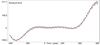Fig. 1 Residuals of ζ6 between the solution of TASS-t ${\Omega }_6^{*}$ and JPL.

5 JPL Representation of the Eccenfricity and the Pericentre of Titan z₆

The calculation for z₆, the eccentricity andpericentre of Titan, is simpler than that of ζ₆. The involved proper frequencies are more accurate. As in the previous section, we remove the short terms and semi-long terms firs8, and then we determine their long terms by a simplified LSM. The solution is listed in Table 9. The mean of the residuals between XA-JPL and JPL is about −213.89 m, and the standard deviation is about 3.53 km.

A comparison between TASS-t and XA-JPL is shown in Table 8. The biggest dieference comet from the major term, the pericentre of Titan ${\varpi }_6^{*}$, of about 86 km in the amplitude. The other differences are smaller than 10 km. XA-JPL is very close to TASS on the eccentricity and pericentre z₆.

6 JPL Representation of the Semi-major Axis a₆ of Titan

The representation of the semi-major axis a₆ is directly obtained by frequency analysis. The main components of a6 in TASS and JPL are similar. XA-JPL has numerous small-amplitude short terms, whose amplitudes reach several hundred metres. The representation of the semi-major axis is listed in Table 10.

7 Updated JPL Representation of the Mean Longitude λ₆ of Titan

An update of the mean longitude λ₆ is calculated, inspired by the discovery of new small-amplitude short terms listed above. Its components have increased from 8 to 15 terms, listed in Table 11; the first eight columns consist of the components reported in Paper I, and the last seven columns consist of the new terms obtained in this study.

It is noteworthy that the mean of the residuals between XA-JPL and JPL increases from −13.27 m to 35.45 m; however, the standard deviation decreases from 25.59 km to 12.47 km, compared with the results in Paper I.

8 Synthetic Representation of Titan

Here, we give a complete analytical representation of all the osculating elements of Titan from JPL: a₆ is the semi-major axis in Table 10; λ₆ is the mean longitude in Table 11; z₆ is the eccentricity and the pericentre in Table 9; and ζ₆ is the inclination and the ascending node in Table 7. The representations of Titan are composed of all these tables, and are named XA-JPL. The corresponding software to compute the orbital elements with these tables is available on request. The software also can calculate the orbit in the form of position-velocities referring to the equinox and ecliptic J2000 system with Eqs. (2) and (3).

9 Conclusions

In this work, we established a connection between the theoretical ephemerides and the numerical integration ephemerides. We completed the analytical representations of the osculating elements of the JPL Titan ephemeris and obtained most of the proper frequencies related to the representations, consisting of all the major proper frequencies of Titan, including the mean longitude and the ascending node of Rhea and the mean longitude of Enceladus, Tethys, Dione, and Iapetus.

Our representations report the system dynamic information and the detailed perturbation relationship of JPL, which were not clearly exhibited before. The standard deviation between XA-JPL and JPL in position is smaller than 628.19 m, and the mean residual is only several centimetres.

We expect to make further research on the representations of other major Saturn satellites, to get more proper frequencies and dynamic information on the Saturn system. Moreover, we would like to make a similar study on other Saturnian numerical ephemerides like NOE (Lainey et al. 2004a,b), and also on the numerical ephemerides of the satellites of other planet systems, such as the Martian satellites.

Acknowledgements

We thank Melaine Saillenfest for the use of his software of frequency analysis. The authors also thank the reviewer for very useful and helpful comments. X.J. Xi acknowledges a financial support from the National Science Foundation of China (NSFC) (12173042).

Appendix A Extension of the Frequency Analysis Via the Least-squares Method

The calculation of ζ₆ or z₆ is described in this Appendix. It uses the same method for the λ₆ calculation as in Paper I. Considering an integrable Hamilton system with m degrees of freedom based on a Hamiltonian H, if the system evolves within the hypothesis of the Arnold-Liouville theorem, there are some coordinates called action-angles. The action-angle coordinates are intrinsic to the system. The first derivatives of the action variables give the proper frequencies ω_j.

When a function f(t) describes a mechanical system, for example, f(t) may stand for one of the variables in Eq. 2, and it can be written as a series in the form $$f\left(t\right)={\displaystyle \sum _{k\in \text{N}}{A}_k}\exp i{v}_{k}t\text{\hspace{0.17em}with\hspace{0.17em}}{\text{A}}_k\in ℂ,$$(A.1)

where v_j are the integer combinations of the proper frequencies ω_j.

In this paper we assume that the system is integrable, or at least close to integrable. Hence, the corresponding equation of orbital elements can be written as $$Y\left(t\right)={\displaystyle \sum _{i=1}^{n_t}{A}_1,i}co\left(\omega it+{\varphi }_i\right)+\text{ι}\times {\displaystyle \sum _{i=1}^{n_t}{A}_2{,}_i\sin \left({\omega }_{i}t+{\varphi }_i\right),}$$(A.2)

where Y(t) is the value of ζ₆ or z₆ at time t and n_t is the number of the terms.

Each frequency ω can be an integer combination of several proper frequencies, a single frequency itself, or a multiple of a single frequency. The series is considered periodic or quasi-periodic. It is constructed following the D’Alembert rule (Laskar et al. 1992; Laskar 1993), where ϕ_i and A_i are the phase and amplitude related to ω_i.

In the case of the mean longitude, λ₆ has only a real part: $$Y\left(t\right)={\displaystyle \sum _{i=1}^{n_t}{A}_1{,}_i\sin \left({\omega }_{i}t+{\varphi }_i\right)}.$$(A.3)

The complete representation of the mean longitude needs to add its main slope Nt and initiate λ₀: $$\lambda =N_t+{\lambda }_0+{\displaystyle \sum _{i=1}^{n_t}{A}_1}{,}_i\sin \left({\omega }_{i}t+{\varphi }_i\right).$$(A.4)

Their unknown amplitudes and phases are determined by the LSM. The semi-major axis a₆ has only a real part. It is not considered in the LSM as its representation can be obtained directly by frequency analysis.

With a step of 0.6 days over 1000 year, we have m = 607800 equations for each osculating element of Titan. If we use $$\begin{array}{ccc}\sin \left({\omega }_1{t}_i\right)& =& X_{i,1}\\ \cos \left({\omega }_1{t}_i\right)& =& X_{i,2}\\ \sin \left({\omega }_1{t}_i\right)& =& X_{i,3}\\ & & \dots \\ \cos \left({\omega }_n{t}_i\right)& =& X_{n,n}\end{array}$$(A.5) $$\{\begin{array}{lll}{a}_1{{}_{,}}_1\hfill & =\hfill & A_1\sin {\varphi }_1\hfill \\ a_2{{}_{,}}_1\hfill & =\hfill & A_1\cos {\varphi }_1\hfill \\ a_1{{}_{,}}_2\hfill & =\hfill & A_1\cos {\varphi }_1\hfill \\ a_{2,2}\hfill & =\hfill & -A_1\sin {\varphi }_1\hfill \\ a_{1,3}\hfill & =\hfill & A_2\sin {\varphi }_2\hfill \\ a_{2,3}\hfill & =\hfill & A2\cos {\varphi }_2\hfill \\ a_{1,4}\hfill & =\hfill & A_2\cos {\varphi }_2\hfill \\ a_{2,4}\hfill & =\hfill & -A_2\sin {\varphi }_2\hfill \\ \dots \hfill & \hfill & \hfill \end{array}$$(A.6)

then equations are as follows: $$\begin{array}{ccc}X\times A& =& y,\\ X\times A^{*}& =& y^{*}.\end{array}$$(A.7)

Here X is a [m × n] matrix of equations, A and A* are unknown one-dimensional matrices, n_t is the number of terms, and n is the number of parameters, which is twice n_t. The phase and amplitude remain constant throughout. The difference between the equations depends on the time t and the corresponding Y(t). Here $$\begin{array}{l}X\hfill \\ =\left(\begin{array}{cccc}{\displaystyle {\sum }_{i=1}^m{X}_{i,1}^2}& {\displaystyle {\sum }_{i=1}^m{X}_{i,1}}{X}_{i,2}\dots & {\displaystyle {\sum }_{i=1}^m{X}_{i,1}{X}_{i,n-1}}& {\displaystyle {\sum }_{i=1}^m{X}_{i,1}{X}_{i,n}}\\ ⋮& ⋮& ⋮& ⋮\\ {\displaystyle {\sum }_{i=1}^m{X}_{i,n}{X}_{i,1}}& {\displaystyle {\sum }_{i=1}^m{X}_{i,n}{X}_{i,2}}\dots & {\displaystyle {\sum }_{i=1}^m{X}_{i,n}{X}_{i,n-1}}& {\displaystyle {\sum }_{i=1}^m{X}_{i,n}^2}\end{array}\right),\hfill \\ \mathcal{A}=\left(\begin{array}{c}{a}_{1,1}\\ ⋮\\ a_{1,n}\end{array}\right),\hfill \\ {\mathcal{A}}^{*}=\left(\begin{array}{c}{a}_{2,1}\\ ⋮\\ a_{2,n}\end{array}\right),\hfill \\ \mathcal{Y}=\left(\begin{array}{c}{\displaystyle {\sum }_{i=1}^m{X}_{2i-1}{,}_1{Y}_{2i-1,t2i-1}}\\ ⋮\\ {\displaystyle {\sum }_{i=1}^m{X}_{2i-1,m}}{Y}_{t2i-1}\end{array}\right),\hfill \\ {\mathcal{Y}}^{*}=\left(\begin{array}{c}{\displaystyle {\sum }_{i=1}^m{X}_{2i-1}{Y}_{t2i}}\\ ⋮\\ {\displaystyle {\sum }_{i=1}^m{X}_{2i,m}{Y}_{t2i}}\end{array}\right).\hfill \end{array}$$

For λ₆ we only use the first equation in Eq. A.7.

References

All Tables

All Figures

	Fig. 1 Residuals of ζ6 between the solution of TASS-t ${\Omega }_6^{*}$ and JPL.
In the text

References

- Duriez, L. 1977, A&A, 54, 93 [NASA ADS] [Google Scholar]
- Duriez, L. 1979, PhD Thesis, Université de Lille, France [Google Scholar]
- Giorgini, J. D., Yeomans, D. K., Chamberlin, A. B., et al. 1996, Bull. Am. Astron. Soc., 28, 1158 [Google Scholar]
- Jet Propulsion Laboratory (JPL) 2018, HORIZONS Web-Interface, https://ssd.jpl.nasa.gov/?horizons/ [Google Scholar]
- Lainey, V., Arlot, J. E., & Vienne, A. 2004a, A&A, 420, 1171 [NASA ADS] [CrossRef] [EDP Sciences] [Google Scholar]
- Lainey, V., Duriez, L., & Vienne, A. 2004b, A&A, 427, 371 [NASA ADS] [CrossRef] [EDP Sciences] [Google Scholar]
- Laskar, J. 1993, Physica D: Nonlinear Phenomena, 67, 257 [NASA ADS] [CrossRef] [Google Scholar]
- Laskar, J., Froeschlé, C., & Celletti, A. 1992, Physica D: Nonlinear Phenomena, 56, 253 [NASA ADS] [CrossRef] [Google Scholar]
- Saillenfest, M. 2014, Représentation synthétique du mouvement des satellites de Saturn, Report of Paris Observatory [Google Scholar]
- Vienne, A. 1991, Thesis, Université de Lille, France [Google Scholar]
- Vienne A., & Duriez, L. 1991, A&A, 246, 619 [NASA ADS] [Google Scholar]
- Vienne, A., & Duriez, L. 1995, A&A, 297, 588 [NASA ADS] [Google Scholar]
- Xi, X. J. 2018, Thesis, Observatoire de Paris, Université PSL, France [Google Scholar]
- Xi, X. J., & Vienne, A. 2020, A&A, 635, A91 [NASA ADS] [CrossRef] [EDP Sciences] [Google Scholar]