| Issue |
A&A
Volume 663, July 2022
|
|
|---|---|---|
| Article Number | A69 | |
| Number of page(s) | 7 | |
| Section | Numerical methods and codes | |
| DOI | https://doi.org/10.1051/0004-6361/202142626 | |
| Published online | 19 July 2022 | |
ShapeNet: Shape constraint for galaxy image deconvolution
1
AIM, CEA, CNRS, Université Paris-Saclay, Université de Paris,
91191
Gif-sur-Yvette, France
e-mail: This email address is being protected from spambots. You need JavaScript enabled to view it.
This email address is being protected from spambots. You need JavaScript enabled to view it.
2
Laboratoire d’astrophysique, École Polytechnique Fédérale de Lausanne (EPFL),
Switzerland
e-mail: This email address is being protected from spambots. You need JavaScript enabled to view it.
3
LESIA, Observatoire de Paris, Université PSL, CNRS, Sorbonne Université, Université de Paris,
5 place Jules Janssen,
92195
Meudon, France
4
Université Paris-Saclay, CEA, CNRS, Inserm, BioMAPs,
91401
Orsay, France
5
Wisear,
11 rue des Cassoirs,
89000
Auxerre, France
Received:
9
November
2021
Accepted:
31
March
2022
Abstract
Deep learning (DL) has shown remarkable results in solving inverse problems in various domains. In particular, the Tikhonet approach is very powerful in deconvolving optical astronomical images. However, this approach only uses the ℓ2 loss, which does not guarantee the preservation of physical information (e.g., flux and shape) of the object that is reconstructed in the image. A new loss function has been proposed in the framework of sparse deconvolution that better preserves the shape of galaxies and reduces the pixel error. In this paper, we extend the Tikhonet approach to take this shape constraint into account and apply our new DL method, called ShapeNet, to a simulated optical and radio-interferometry dataset. The originality of the paper relies on i) the shape constraint we use in the neural network framework, ii) the application of DL to radio-interferometry image deconvolution for the first time, and iii) the generation of a simulated radio dataset that we make available for the community. A range of examples illustrates the results.
Key words: miscellaneous / radio continuum: galaxies / techniques: image processing / methods: data analysis / methods: numerical
© F. Nammour et al. 2022
 Open Access article, published by EDP Sciences, under the terms of the Creative Commons Attribution License (https://creativecommons.org/licenses/by/4.0), which permits unrestricted use, distribution, and reproduction in any medium, provided the original work is properly cited.
1 Introduction
Sparse wavelet regularization, based either on the ℓ0 or ℓ1 norm, has been the commonly approved technique for astronomical image deconvolution for years. It has led to striking results, such as an improvement in resolution by a factor of four (two factors in each dimension) in the Cygnus-A radio image reconstruction compared to the CLEAN standard algorithm (Garsden et al. 2015). Sparsity, similarly to the positivity regularization constraint, can be considered as a weak prior on the distribution of the wavelet coefficients of the solution because most if not all images present a compressible behavior in the wavelet domain. In recent years, the emergence of DL has shown promising results in various domains, including deconvolution (Xu et al. 2014). In astrophysics, methods based on DL have been developed to perform model fitting that can be seen as a parametric deconvolution (Tuccillo et al. 2018). Sureau et al. (2020) introduced the Tikhonet neural network for optical galaxy image deconvolution. Tikhonet clearly outperformed sparse regulariza-tion for the mean square error (MSE) and a shape criterion, the galaxy shape being encoded through a measure of its ellipticity (Sureau et al. 2020). These great results can be explained by the fact that DL learns, or rather approximates, the mean of the posterior distribution of the solution. As there is no guarantee that a nonlinear deconvolution process preserves the galaxy shapes, Nammour et al. (2021) introduced a new shape penalization term and showed that the addition of this penalty to sparse regularization improves both the solution shape and the MSE. In this paper, we propose a new deconvolution method, called ShapeNet, by extending the Tikhonet method to include the shape constraints. We present first results for optical galaxies image deconvolution and then show that Tikhonet and ShapeNet can also be used in the framework of radio galaxy image deconvolution. To achieve these results, we have developed our own datasets for optical and radio astronomical images. The optical dataset generation uses Hubble Space Telescope (HST)-like target images and simulates Canada France Hawaii telescope (CFHT)-like noisy observations by using real images and point spread functions (PSF) from the coordinates, sizes, magnitudes, orientations, and shapes (COSMOS) catalog (Mandelbaum et al. 2012). The radio dataset comprises noisy images with realistic PSFs similar to those of the MeerKAT telescope, and parametric galaxies with properties taken from the tiered radio extragalactic continuum simulation (T-RECS) catalog (Bonaldi et al. 2019).The optical and radio dataset generation are adapted for machine learning, and theyare explained in Appendices A.1 and A.2, respectively. Section 2 introduces our new method, and Sect. 3 presents the results of numerical experiments. We conclude in Sect. 4.
2 Deep-learning deconvolution with a shape constraint
2.1 Deconvolution problem
When we denote the observed image by y ∊ Rn☓n and the PSF by h ∊ Rn☓n, the observational model is
 (1)
(1)
where xT ∊ Rn☓n is the ground-truth image, and n ∊ Rn☓n is additive noise. We can partially restore y by applying the least-squares method. In this case, the solution oscillates because the problem in Eq. (1) is ill conditioned. More generally, it is an ill-posed problem and can instead be tackled using regulariza-tion (Bertero & Boccacci 1998). For example, when we note the circulant matrix corresponding to the convolution operator h as H e ∊ Rn☓n, the Tikhonov solution of Eq. (1) is
 (2)
(2)
where is the Tikhonov linear filter, and λ ∊ R+ is the regularization weight.
2.2 Tikhonet deconvolution
The Tikhonet is a two-step DL approach for solving deconvolu-tion problems. The first step is to perform deconvolution using a Tikhonov filter with a quadratic regularization and setting Γ = Id, leading to a deconvolved image containing correlated additive noise that is filtered in a second step using a four-scale XDense U-Net (Sureau et al. 2020). The network is trained to learn the mapping between the Tikhonov output and the target image using the mean square error (MSE) as a loss function. The regularization weight is estimated for each image using a Stein's unbiased risk estimate (SURE) risk minimization with an estimate of the image signal to noise ratio (S/N).
2.3 Shape constraint
The shape information of galaxies is essential in various fields of astrophysics, such as galaxy evolution and cosmology. The measure that is used to study the shape of a galaxy is the ellip-ticity, which is a complex scalar, e = e1 + ie2. The ellipticity of an image x is given by (Kaiser et al. 1995)
 (3)
(3)
where µs,t are the image-centered moments of order (s + t), defined as
![Mathematical equation: ${\mu _{s,t}}\left( x \right) = \sum\limits_{i = 1}^n {\sum\limits_{j = 1}^n {x\left[ {\left( {i - 1} \right)n + j} \right]} {{\left( {i - {i_c}} \right)}^s}{{\left( {j - {j_c}} \right)}^t},} $](/articles/aa/full_html/2022/07/aa42626-21/aa42626-21-eq4.png) (4)
(4)
and ic and jc are the coordinates of the centroid of x, such that
![Mathematical equation: ${i_c} = {{\sum\nolimits_{i = 1}^n {\sum\nolimits_{j = 1}^n {i \cdot x\left[ {\left( {i - 1} \right)n + j} \right]} } } \over {\sum\nolimits_{i = 1}^n {\sum\nolimits_{j = 1}^n {x\left[ {\left( {i - 1} \right)n + j} \right]} } }}$](/articles/aa/full_html/2022/07/aa42626-21/aa42626-21-eq5.png) (5)
(5)
and
![Mathematical equation: ${j_c} = {{\sum\nolimits_{i = 1}^n {\sum\nolimits_{j = 1}^n {j \cdot x\left[ {\left( {i - 1} \right)n + j} \right]} } } \over {\sum\nolimits_{i = 1}^n {\sum\nolimits_{j = 1}^n {x\left[ {\left( {i - 1} \right)n + j} \right]} } }}.$](/articles/aa/full_html/2022/07/aa42626-21/aa42626-21-eq6.png) (6)
(6)
In Nammour et al. (2021), we derived the following reformulation:
 (7)
(7)
and
 (8)
(8)
where are constant images, defined for all as
![Mathematical equation: $\matrix{ {{u_1}\left[ {\left( {i - 1} \right)n + j} \right] = i,} \hfill & {{u_2}\left[ {\left( {i - 1} \right)n + j} \right] = j,} \hfill \cr {{u_3}\left[ {\left( {i - 1} \right)n + j} \right] = 1,} \hfill & {{u_4}\left[ {\left( {i - 1} \right)n + j} \right] = \left( {{i^2} + {j^2}} \right),} \hfill \cr {{u_5}\left[ {\left( {i - 1} \right)n + j} \right] = \left( {{i^2} - {j^2}} \right),} \hfill & {{u_6}\left[ {\left( {i - 1} \right)n + j} \right] = \left( {ij} \right).} \hfill \cr } $](/articles/aa/full_html/2022/07/aa42626-21/aa42626-21-eq9.png) (9)
(9)
All the scalar products in Eqs. (7) and (8) are linear in x. Therefore, by formulating the shape constraint as a data-fidelity term in this scalar product space, we obtain
 (10)
(10)
where {ω1,…,ω6} are non-negative scalar weights. Equation (10) offers a shape constraint whose properties are straightforwardly derived. However, the ellipticity measure is extremely sensitive regarding noise. To add robustness to the shape constraint, we considered windowing the observed image, y, to reduce the noise effect. One approach is to fit a Gaussian window on y, but this would require an additional preprocessing step in each observed image. To avoid this step, we chose to use a set of precomputed windows such that at least one of them fits the galaxy in the observed image. We considered curvelets to determine a candidate set because they are a family of linear multiscale transforms that is usually designed with specific properties to efficiently represent objects of interest. This led us to
 (11)
(11)
where {ωij}ij are non-negative scalar weights (their computation is detailed in Nammour et al. (2021)), and {ψj}j are K -directional and multiscale filters, derived from a curvelet-like decomposition (Starck et al. 2015; Kutyniok & Labate 2012). These filters allow capturing the anisotropy of the galaxy image and are used in the constraint as a set of windows such that at least one of them reduces the noise in the image and emphasizes the useful signal. We have also shown that adding such a constraint to a sparse deconvolution approach reduces both the shape and pixel errors (Nammour et al. 2021). An alternative could have been to directly use the ellipticity in the loss function rather than our shape constraint. However, this would have raised some serious issues. The ellipticity measurement is very sensitive to noise, and it would have been necessary to take the noise propagation on the ellipticity measurements into account. As the propagated noise would clearly not be Gaussian, this is far from being trivial. Furthermore, the ellipticity operator is nonlinear in x, which complicates the gradient computation, thus rendering optimization much more difficult. In contrast, our shape constraint is the sum of weighted-squared fully linear components, and the noise can be well controlled.
2.4 ShapeNet deconvolution
This shape constraint can also be used in a DL deconvolution framework by extending the Tikhonet method. We propose here the ShapeNet DL deconvolution, which applies the following updates to Tikhonet: First, we set Γ to a Laplacian filter instead of the identity. This is motivated by the fact that images have generally a decreasing profile in Fourier space and the data quality at high frequencies is more deteriorated than at low ones.
Second, the weight of the regularization parameter λ is constant for all images, which adds homogeneity to the filter in the ShapeNet pipeline and improves the explainability of the task learned by the XDense U-Net. Third, the loss function used to train the network contains an additional term, which is the shape constraint.
The loss function is now expressed as
 (12)
(12)
where is the Tikhonov filter output of the observed image, M is the shape constraint, and γ ∊ R+ is its weight parameter as introduced in Nammour et al. (2021). The choice of the hyperparameters is detailed in Appendices B.1 and B.2.
3 Numerical experiments and results
In this section, we present the numerical experiments we carried out in order to assess the methods discussed above. The code was developed using Python 3.7.5 and TensorFlow 1.15.2, Keras 2.3.1 (Chollet 2015), AlphaTransform1, Matplotlib 3.1.3 (Hunter 2007), Galaxy2Galaxy, and GalFlow (Lanusse & Remy 2019). While training the U-Net for the DL methods with and without a shape constraint, we normalized the pixel values of the input images by 4 × 10³ for the optical case and by 2 × 10³ for the radio case in order to make their magnitudes close to unity, so that the activation functions in the neural network could distinguish the data better. We compared the DL methods to sparse reconstruction algorithm (SRA) and shape constraint restoration algorithm (SCORE) (Nammour et al. 2021), and additionally, to CLEAN for the radio case. SRA is a deconvolution method based on sparsity and positivity, while SCORE is its extension and uses an additional shape constraint, as described in Nammour et al. (2021). The qualitative criteria used for these experiments are listed below.

Relative error of the flux density:

Mean absolute error of each component of the ellipticity: e1 and e2.
The ellipticity in this case was estimated using the adaptive moments method (Hirata & Seljak 2003), which consists of fitting an elliptical Gaussian window on the input image and then deducing the measurement from the window obtained.
3.1 Optical experiments
For the optical experiments, we used the CFHT2HST dataset, whose implementation is detailed in Appendix B.1. For visual comparison, we show five examples of resolved galaxies in Fig. 1. First, we observe that the sparse methods tend to make the reconstructed object more isotropic and smoother, noting that the fine details present in the ground truth are lost during reconstruction. This effect is explained by the use of starlets, which are isotropic wavelets. The DL methods preserve more details and structures, as seen for the first galaxy. When the shape constraint is added, whether going from SRA to SCORE or from Tikhonet to ShapeNet, there is a better coincidence between the orientation of the reconstructed galaxies and the ground truth. We also note that the addition of the shape constraint allows a better reconstruction of large galaxies. This can be seen for the Tikhonet results, where galaxies reconstructed without the constraint appear to be smaller and less bright than the ground truth at a significant noise level.
To measure the MSE, we carried out a weighting with the elliptical Gaussian window obtained while estimating the ground-truth galaxy shape. This weighting reduces the noise in the ground-truth images, allowing us to reduce the bias in the estimation of MSE. Quantitatively, we also compared sparse methods to DL methods by taking SRA and Tikhonet. Our results corroborate those of Sureau et al. (2020), that is, in almost all measurements listed in Table 1 and shown in Fig. 2, Tikhonet average errors are lower than those obtained with SRA. We note that for both methods, sparsity and neural network, adding the shape constraint reduces the errors. In Table 1, the ShapeNet reconstructions again have lower errors than those obtained with Tikhonet, with reductions of 26%, 48%, 6%, and 5% for MSE, flux, e1, and e2, respectively. Thus, we show that the addition of the shape constraint improves the performance of the methods considered with respect to all the quality criteria studied, which corroborates the results in Nammour et al. (2021). In conclusion, the experiments carried out on the CFHT2HST dataset show that adding the shape constraint in a DL framework significantly reduces the reconstruction errors.
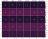 |
Fig. 1 Examples of extended galaxies reconstructed using the CFHT2HST dataset. |
CFHT2HST dataset results.
3.2 Radio experiments
So far, DL deconvolution methods have only been tested on optical data. In this section, we extend the results of Sureau et al. (2020) by first investigating how DL techniques perform for radio galaxy deconvolution, and we then add a shape constraint during the neural network training. For the radio experiments, we used the MeerKAT3600 dataset, whose implementation is detailed in Appendix B.2. In Fig. 3 we show examples of galaxies where the peak signal to noise ratio (PSNR) is greater than 3, so that we can distinguish galaxies from noise in observations. The CLEAN and sparse-recovered images are both smoother than the corresponding ground truths, and the orientation of the reconstructed galaxies is strongly biased by that of the PSF. Deep-learning methods better preserve details such as shape, size, and orientation. Deep-learning methods are able to detect galaxies even when the PSNR is extremely low (as shown in the last column of Fig. 3). Furthermore, the shape constraint helps to noticeably improve the results for galaxies with PSNR greater than 10 as shown in Fig. 4.
Similar to the optical case, adding the shape constraint to both sparse and DL methods improves their performance in the radio case as well. In more detail, Table 2 shows that the ShapeNet reconstructions have lower errors than those obtained with Tikhonet, with reductions of 17%, 7%, 1%, and 2% for MSE, flux, e1, and e2, respectively.
We finally conclude that the sparsity and DL methods perform better than CLEAN, adding the shape constraint brings a gain in all the quality criteria considered, and DL offers a better performance than sparsity. Finally, ShapeNet outperforms all other methods discussed above.
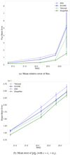 |
Fig. 2 Mean errors of reconstruction as a function of magnitude for the CFHT2HST dataset, where the error bars correspond to the standard error of the given value. |
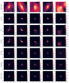 |
Fig. 3 Examples of galaxies with PSNR greater than 3, reconstructed from the MeerKAT3 600 dataset. |
MeerKAT3600 dataset results.
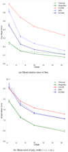 |
Fig. 4 Mean errors of reconstruction as a function of PSNR for the MeerKAT3600 dataset. |
4 Conclusion
We have introduced ShapeNet, a new problem-specific approach, based on optimization and DL, to solve the galaxy deconvolution problem. We developed and generated two realistic datasets that we adapted for our numerical experiments, in particular, the training step in DL. Our work extends the results of Sureau et al. (2020) by first investigating how DL techniques behave for radio-interferometry galaxy image deconvolution, and then adding a shape constraint during the neural network training. Our experiments have shown that the Tikhonet and ShapeNet DL deconvolution methods allow us to better reconstruct radio-interferometry image reconstructions. We have shown that the shape constraint improves the performance of galaxy deconvolution for optical and radio-interferometry images for different criteria, such as the pixel error, the flux, and the ellipticity. In practice, this method can be used with a source-extraction algorithm to restore wide-field images containing multiple galaxies.
We will evaluate our method on real data. ShapeNet might be improved by replacing the U-Net by a more competitive denoiser such as the deep iterative down-up CNN for image denoising (DIDN) (Yu et al. 2019) or Laine et al. (2019) method. Additionally, ShapeNet might also be improved by adding filters to extract feature maps before the deconvolution step in a similar fashion to Dong et al. (2021). We are currently investigating the addition of the shape constraint to an ameliorated version of the ADMM-net method presented in Sureau et al. (2020). The amelioration concerns the properties of the neural network that are discussed in Pesquet et al. (2021). On a wider scope, our deconvolution method can also be applied to other fields that will be addressed by the square kilometre array (SKA). An efficient deconvolution method that is accessible to the community enables reconstructing a better estimate of the sky with fewer data than classical methods. This is key for optimizing the observing time and the number of required data to achieve a given image reconstruction fidelity. In the upcoming surveys involving SKA 1-MID, the use of DL methods that are specific to the behavior of an instrument during an observation will be critical to limit the deluge of data produced by the new generation of radio interferometers.
Acknowledgements
We would like to thank Axel Guinot and Hippolyte Karakostanoglou for their valuable help implementing the optical dataset.
Appendix A Generating the datasets
For DL, a huge and realistic dataset is required to obtain relevant results. The codes we used to generate our datasets are written in Python 3.6, use GalSim (Rowe et al. 2015), TensorFlow 1.15.2, and are publicly available on GitHub (see Appendix C). The noise is added on the go and is adjusted according to the application.
Appendix A.1: Optical dataset
We developed the CFHT2HST dataset such that the target images are HST-like and the input images are CFHT-like. The dataset consists of the following:
Target galaxy, also called ground-truth galaxy. This galaxy is obtained by convolving a real HST galaxy image from the COSMOS catalog (Mandelbaum et al. 2012) with the target PSF to reach a determined target resolution.
Target PSF. The role of this PSF is to limit the resolution of the target galaxy to obtain a realistic simulation of an image observed by a telescope. The target PSF is unique because its variations are negligible with respect to the input PSF.
Input galaxy. The image is obtained by convolving the image from the COSMOS catalog with the input PSF, and adding noise with a constant standard deviation for all images. The value of the standard deviation is computed by taking the conditions of observation and the properties of the CFHT telescope2
 [URL] into account.
Input PSF. This PSF is used to obtain the input galaxy. It was generated using a Kolmogorov model (Racine 1996).
The characteristics of this dataset are given in Table A.1.
Characteristics of the CFHT2HST dataset.
Appendix A.2: Radio dataset
To our knowledge, no public radio dataset of this magnitude that is suitable for our working environment is available. We therefore developed our own dataset, which is composed of over 50,000 images with realistic PSFs similar to those of the MeerKAT telescope (a precursor to the SKA) at a central frequency of 3600MHz, and parametric galaxies with realistic properties taken from the T-RECS catalog (Bonaldi et al. 2019). The key point to note here is that the noise is masked by the PSF in Fourier space. The noise level is measured in terms of the PSNR, and is defined as the ratio of the maximum useful signal to the standard deviation of the noise (a commonly used convention in radio astronomy).
The generated dataset contains pairs of galaxies and PSFs, the characteristics of which are listed in Table A.2. We use simulated realizations of observational PSFs from the MeerKAT telescope for typical observation times of 2 hours. The PSF is completely determined by i) the observation wavelength, ii) the integration time of the observation, and iii) the distribution of the antennas as seen from the source during the observation. To simulate a variety of realistic cases, we generated integrated PSF realizations over 2 hours for random source directions. A longer observation time allows accumulating more varied samples in the Fourier plane, which decreases artifacts due to incompleteness of the sample mask.
Characteristics of the simulated MeerKAT3600dataset.
Appendix B Implementation
Appendix B.1: Optical dataset
For the optical experiments, we considered the CFHT2HST dataset presented in Appendix A.1. In the same spirit as the experiments carried out in (Sureau et al. 2020), the goal is to reconstruct high-resolution images from low-resolution images, with each resolution corresponding to a telescope. In our case, the high-resolution images correspond to real images from the HST telescope, and the low-resolution images correspond to simulated images at the resolution of the CFHT obtained by degrading the HST images. These are considered the ground truths, and the CFHT images are the observed images. To measure the quality of the signal in the image, we used the absolute magnitude. The noise level added to the latter is constant background noise, which was calculated from the parameters of the telescope3. Therefore, the absolute magnitude up to a multiplicative constant is the opposite of the logarithm of the S/N. We considered four classes of magnitudes, each with an average of 20.79, 22.16, 22.83, and 23.30, and each containing an equal number of samples. The dataset contains point-like galaxies, which are very small and hard to resolve by the telescope. Because measuring the shape of these galaxies is problematic, we removed galaxies from our analysis for which the shape measurement on the ground-truth image had failed. In each class of magnitudes, we then had about 500 galaxies. The studied methods are SRA and SCORE for sparse methods and Tikhonet and ShapeNet for DL. In these last two, the U-net we used contains four scales and was trained over ten epochs composed of 625 steps each, and the batches had a size of 128 each. For the choice of the shape constraint weight in the ShapeNet method, we performed a linear search and found the value γ = 0.5. In the case of SCORE, the weight was set to γ = 1 based on our previous findings in Nammour et al. (2021). In addition, the convolution kernel used in SCORE was obtained by performing a division in Fourier space of the transform of the input PSF by the output one. We then performed a partial deconvolution.
Appendix B.2: Radio dataset
For the radio experiments, we used the MeerKAT3600 dataset presented in Appendix A.2. Unlike in the optical case, ground-truth radio images are realistic, but are not real. They are simulated images using the T-RECS catalog (Bonaldi et al. 2019), and their resolution is not limited by the telescope dirty beam. However, observations were simulated so that they were similar to those of the MeerKAT telescope. To do this, we used the realistic simulation code that we developed using galaxy2galaxy4. The noise level used for these experiments was constant and was chosen so as to obtain a variety of levels of S/N in order to have a broad assessment of the different methods we examined. We used PSNR to quantify the signal quality. We considered four PSNR classes each with an average of 4.38, 6.92, 9.99, and 16.74, containing an equal number of samples. The methods we compared are CLEAN isotropic, SRA, SCORE, Tikhonet, and ShapeNet. We only considered CLEAN isotropic in our comparisons (and denote it as CLEAN) because it is an improvement of the original CLEAN algorithm and allows a fairer comparison with other methods. The dataset contains observations with a very low PSNR that extends below 3, which corresponds to the signal detection threshold for CLEAN. In the subset chosen to perform numerical experiments, 72 out of 3072 galaxies were removed because their PSNR was below the threshold. In the end, we had 750 galaxies per class of PSNR. For the DL, the U-Net we used contains four scales and was trained for ten epochs, with 3125 steps per epoch and a batch size of 32. For the choice of weighting for the shape constraint, we found the value γ = 0,5 for ShapeNet and γ = 2 for SCORE using a linear search. The value of the regularization weight for the Tikhonov filter we used is 9 × 10⁻³ and was also found using a linear search (link to the notebook5: ) [URL] Moreover, for these experiments, we also modified the initialization of the sparse methods, SRA and SCORE, by replacing the constant image by a Tikhonov filtering applied to the observation.
Appendix C Reproducible research
For the sake of reproducible research, all the codes and the data used for this article have been made publicly available online. GitHub pages are indicated with the hyperlink icon and other web pages with  .
.
The branch of the GitHub repository for
Scripts for building and training Tikhonet and ShapeNet8:
[URL],Evaluating the trained network for different shape constraint parameters9:
[URL]
References
- Bertero, M., & Boccacci, P. 1998, Introduction to Inverse Problems in Imaging (CRC Press) [CrossRef] [Google Scholar]
- Bonaldi, A., Bonato, M., Galluzzi, V., et al. 2019, Astrophysics Source Code Library [1906.008] [Google Scholar]
- Chollet, F. 2015, Keras, https://github.com/keras-team/keras/ [Google Scholar]
- Dong, J., Roth, S., & Schiele, B. 2021, ArXiv e-prints [arXiv:2103.09962] [Google Scholar]
- Garsden, H., Girard, J. N., Starck, J. L., et al. 2015, A&A, 575, A90 [CrossRef] [EDP Sciences] [Google Scholar]
- Hirata, C., & Seljak, U. 2003, MNRAS, 343, 459 [Google Scholar]
- Hunter, J. D. 2007, Comput. Sci. Eng., 9, 90 [NASA ADS] [CrossRef] [Google Scholar]
- Kaiser, N., Squires, G., & Broadhurst, T. 1995, ApJ, 449, 460 [Google Scholar]
- Kutyniok, G., & Labate, D. 2012, in Shearlets (Springer), 1 [Google Scholar]
- Laine, S., Karras, T., Lehtinen, J., & Aila, T. 2019, Adv. Neural Informa. Process. Syst., 32 [Google Scholar]
- Lanusse, F., & Remy, B. 2019, GalFlow, https://github.com/DifferentiableUniverseInitiative/GalFlow [Google Scholar]
- Mandelbaum, R., Hirata, C. M., Leauthaud, A., Massey, R. J., & Rhodes, J. 2012, MNRAS, 420, 1518 [NASA ADS] [CrossRef] [Google Scholar]
- Nammour, F., Schmitz, M. A., Mboula, F. M. N., Starck, J.-L., & Girard, J. N. 2021, J. Fourier Anal. Appl., 27, 88 [CrossRef] [Google Scholar]
- Pesquet, J.-C., Repetti, A., Terris, M., & Wiaux, Y. 2021, SIAM J. Imaging Sci., 14, 1206 [CrossRef] [Google Scholar]
- Racine, R. 1996, PASP, 108, 699 [NASA ADS] [CrossRef] [Google Scholar]
- Rowe, B. T. P., Jarvis, M., Mandelbaum, R., et al. 2015, Astron. Comput., 10, 121 [Google Scholar]
- Starck, J.-L., Murtagh, F., & Fadili, J. 2015, Sparse Image and Signal Processing: Wavelets and Related Geometric Multiscale Analysis (Cambridge University Press) [Google Scholar]
- Sureau, F., Lechat, A., & Starck, J. L. 2020, A&A, 641, A67 [NASA ADS] [CrossRef] [EDP Sciences] [Google Scholar]
- Tuccillo, D., Huertas-Company, M., Decencière, E., et al. 2018, MNRAS, 475, 894 [NASA ADS] [CrossRef] [Google Scholar]
- Xu, L., Ren, J. S., Liu, C., & Jia, J. 2014, in Advances in Neural Information Processing Systems, eds. Z. Ghahramani, M. Welling, C. Cortes, N. Lawrence, & K. Q. Weinberger, 27 [Google Scholar]
- Yu, S., Park, B., & Jeong, J. 2019, in Proceedings of the IEEE Conference on Computer Vision and Pattern Recognition Workshops [Google Scholar]
For more details on generation of the observed galaxies and calculation of the noise level see: https://github.com/CosmoStat/ShapeDeconv/blob/master/data/CFHT/HST2CFHT.ipynb
For more details on simulating realistic MeerKAT images with the T-RECS catalog, see: https://github.com/CosmoStat/ShapeDeconv/blob/master/data/T-RECS/Generate%20Radio% 20ground%20truth%20from%20T-RECS.ipynb
All Tables
All Figures
|
Fig. 1 Examples of extended galaxies reconstructed using the CFHT2HST dataset. |
| In the text | |
|
Fig. 2 Mean errors of reconstruction as a function of magnitude for the CFHT2HST dataset, where the error bars correspond to the standard error of the given value. |
| In the text | |
|
Fig. 3 Examples of galaxies with PSNR greater than 3, reconstructed from the MeerKAT3 600 dataset. |
| In the text | |
|
Fig. 4 Mean errors of reconstruction as a function of PSNR for the MeerKAT3600 dataset. |
| In the text | |
Current usage metrics show cumulative count of Article Views (full-text article views including HTML views, PDF and ePub downloads, according to the available data) and Abstracts Views on Vision4Press platform.
Data correspond to usage on the plateform after 2015. The current usage metrics is available 48-96 hours after online publication and is updated daily on week days.
Initial download of the metrics may take a while.