| Issue |
A&A
Volume 662, June 2022
|
|
|---|---|---|
| Article Number | A104 | |
| Number of page(s) | 13 | |
| Section | Interstellar and circumstellar matter | |
| DOI | https://doi.org/10.1051/0004-6361/202142931 | |
| Published online | 24 June 2022 | |
SOLIS
XVI. Mass ejection and time variability in protostellar outflows: Cep E
1
Univ. Grenoble Alpes, CNRS, IPAG,
38000
Grenoble,
France
e-mail: This email address is being protected from spambots. You need JavaScript enabled to view it.
2
Laboratoire de Physique de l’ENS, ENS, Université PSL, CNRS, Sorbonne Université, Université de Paris,
75005
Paris,
France
3
Observatoire de Paris, PSL University, Sorbonne Université, LERMA,
75014
Paris,
France
4
Max-Planck-Institut für extraterrestrische Physik,
Giessenbachstrasse 1,
85748
Garching,
Germany
5
Department of Astronomy, The University of Texas at Austin,
2500 Speedway,
Austin,
TX
78712,
USA
6
Institut de Radioastronomie Millimétrique (IRAM),
300 rue de la Piscine,
38406
Saint-Martin-D’Hères,
France
7
INAF, Osservatorio Astrofísico di Arcetri,
Largo E. Fermi 5,
50125
Firenze,
Italy
8
Leiden Observatory, Leiden University,
PO Box 9513,
2300 RA
Leiden,
The Netherlands
9
Department of Physics and Astronomy, University College London,
Gower Street,
London
WC1E 6BT,
UK
10
IGN, Observatorio Astronómico Nacional,
Calle Alfonso XII,
28004
Madrid,
Spain
11
Dipartimento di Chimica, Biologia e Biotecnologie,
Via Elce di Sotto 8,
06123
Perugia,
Italy
12
Dipartimento di Chimica “G. Ciamician”
via F. Selmi 2,
40126
Bologna,
Italy
13
Université de Toulouse, UPS-OMP, IRAP,
Toulouse,
France
14
CNRS, IRAP,
9 Av. Colonel Roche, BP 44346,
31028
Toulouse Cedex 4,
France
15
LERMA, Université de Cergy-Pontoise, Observatoire de Paris, PSL Research University, CNRS, Sorbonne Université, UPMC,
Univ. Paris 06,
95000
Cergy Pontoise,
France
16
Departament de Química, Universitat Autónoma de Barcelona,
08193
Bellaterra,
Catalonia,
Spain
17
Centro de Astrobiología (CSIC, INTA),
Ctra. de Ajalvir, km. 4, Torrejón de Ardoz,
28850
Madrid,
Spain
18
University of AL-Muthanna, College of Science, Physics Department,
AL-Muthanna,
Iraq
19
Department of Physics, The University of Tokyo,
7-3-1, Hongo, Bunkyo-ku,
Tokyo
113-0033,
Japan
20
Ural Federal University,
620002,
19 Mira street,
Yekaterinburg,
Russia
21
The Institute of Physical and Chemical Research (RIKEN),
2-1, Hirosawa, Wako-shi,
Saitama
351-0198,
Japan
22
Univ. Rennes, CNRS, IPR (Institut de Physique de Rennes) – UMR 6251,
35000
Rennes,
France
23
ESO,
Karl Schwarzchild Srt. 2,
85478
Garching bei München,
Germany
24
Aix-Marseille Université,
PIIM UMR-CNRS 7345,
13397
Marseille,
France
25
Università degli Studi di Torino, Dipartimento Chimica
Via Pietro Giuria 7,
10125
Torino,
Italy
Received:
16
December
2021
Accepted:
8
March
2022
Abstract
Context. Protostellar jets are an important agent of star formation feedback, tightly connected with the mass-accretion process. The history of jet formation and mass ejection provides constraints on the mass accretion history and on the nature of the driving source.
Aims. We characterize the time-variability of the mass-ejection phenomena at work in the class 0 protostellar phase in order to better understand the dynamics of the outflowing gas and bring more constraints on the origin of the jet chemical composition and the mass-accretion history.
Methods. Using the NOrthern Extended Millimeter Array (NOEMA) interferometer, we have observed the emission of the CO 2–1 and SO NJ = 54–43 rotational transitions at an angular resolution of 1.0″ (820 au) and 0.4″ (330 au), respectively, toward the intermediate-mass class 0 protostellar system Cep E.
Results. The CO high-velocity jet emission reveals a central component of ≤400 au diameter associated with high-velocity molecular knots that is also detected in SO, surrounded by a collimated layer of entrained gas. The gas layer appears to be accelerated along the main axis over a length scale δ0 ~ 700 au, while its diameter gradually increases up to several 1000 au at 2000 au from the protostar. The jet is fragmented into 18 knots of mass ~10−3 M⊙, unevenly distributed between the northern and southern lobes, with velocity variations up to 15 km s−1 close to the protostar. This is well below the jet terminal velocities in the northern (+ 65 km s−1) and southern (−125 km s−1) lobes. The knot interval distribution is approximately bimodal on a timescale of ~50–80 yr, which is close to the jet-driving protostar Cep E-A and ~150–20 yr at larger distances >12″. The mass-loss rates derived from knot masses are steady overall, with values of 2.7 × 10⁻⁵ M⊙ yr−1 and 8.9 × 10⁻⁶ M⊙ yr−1 in the northern and southern lobe, respectively.
Conclusions. The interaction of the ambient protostellar material with high-velocity knots drives the formation of a molecular layer around the jet. This accounts for the higher mass-loss rate in the northern lobe. The jet dynamics are well accounted for by a simple precession model with a period of 2000 yr and a mass-ejection period of 55 yr.
Key words: ISM: jets and outflows / ISM: kinematics and dynamics / stars: formation
NSF Astronomy and Astrophysics Postdoctoral Fellow.
© A. de A. Schutzer et al. 2022
 Open Access article, published by EDP Sciences, under the terms of the Creative Commons Attribution License (https://creativecommons.org/licenses/by/4.0), which permits unrestricted use, distribution, and reproduction in any medium, provided the original work is properly cited.
1 Introduction
The earliest stages of the low-mass star formation process are associated with powerful mass-loss phenomena in the form of high-velocity (~100 km s−1) collimated jets. These jets accelerate the ambient circumstellar gas and drive the formation of low-velocity (~ 10 km s−1) molecular outflows (Raga & Cabrit 1993), commonly observed in the millimeter lines of CO (Bachiller 1996). Although the actual jet launch mechanism is still debated (e.g., Bally 2016), it is well established that mass-loss phenomena take their origin in the inner 1–100 au around the nascent star, and their interaction with the dense surrounding protostellar gas is expected to play a major role in the formation of protostellar jets themselves (Frank et al. 2014). Jet-outflow systems have also been proposed to remove angular momentum from the central protostellar regions and in this way to allow material accretion from the disk onto the central object (Frank et al. 2014). Therefore, the formation of jet-outflow systems seems to be an indispensable mechanism in the process of mass accretion by the protostar. Retrieving the history of the jet may provide some constraints to the mass accretion history.
The time variability of the mass-ejection phenomena associated with young stellar objects was identified a long time ago in studies of Herbig–Haro (HH) objects. These studies revealed knots and wiggling structures. Measurements of the proper motion of HH objects showed direct evidence of velocity variations (Reipurth & Bally 2001). Close to the powering source(s) of the HH jet(s), chains of aligned knots are detected, while at larger distances, disconnected heads with lower velocities trace the impact against the ambient cloud. Raga et al. (1990) showed that velocity variability in the ejection process drives the formation of internal working surfaces, where the fast jet material catches up with the slow material. This results in bright emission knots along the jet, while the ejection direction variability produces a garden-hose effect in which the ejected material diverges from an equilibrium-axis position. The distribution of knot dynamical ages measured in class I atomic jets suggests that there are up to three superposed ejection modes with typical timescales of a few 10 yr, 102 yr, and 103 yr, respectively (Raga et al. 2002).
The wiggling structure observed in molecular outflows has been interpreted and successfully modeled in terms of variability of the ejection direction (see, e.g., Gueth et al. 1996; Eisloeffel et al. 1996; Ferrero et al. 2015; Podio et al. 2016; Lefèvre et al. 2017). Several theoretical models have been proposed to explain this phenomenon (Masciadri & Raga 2002; Terquem et al. 1999; Frank et al. 2014), but direct observational constraints are still lacking. It seems, however, that most of the identified precessing jets arise from multiple protostellar systems, which suggests that the presence of companion(s) probably plays a role in the origin of the phenomenon. The precession periods derived toward class 0/I objects range from ~400 yr to 5 × 10⁴ yr (Frank et al. 2014).
Recently, the IRAM Large Program Continuum And Lines in Young ProtoStellar Objects (CALYPSO) has significantly enhanced the statistics for the properties of molecular protostellar jets and their outflows by targeting a sample of 30 nearby (d < 450 pc) protostellar sources, mainly in the class 0 stage, which were observed in selected millimeter transitions of CO, SiO, and SO (Podio et al. 2021). A high detection rate (>80%) of high-velocity collimated jets was reported for sources with L > 1 L⊙, with a velocity asymmetry between the jet lobes for ~30% of the sample. Interestingly, half of the 12 protostellar jets detected in SiO display evidence for bending axes, which is suggestive of precession or wiggling.
High-angular resolution observations of class 0/I protostellar jets with ALMA and NOEMA, such as HH111, HH212, IRAS 04166+2706, and L1157 (Lefloch et al. 2007; Codella et al. 2007, 2014; Tafalla et al. 2010; Podio et al. 2016; Plunkett et al. 2015), bring strong evidence of time variability of the ejection process in the early protostellar phase. A few observational estimates on timescales have been obtained, as illustrated by Plunkett et al. (2015), who reported an average value of 310 ± 150 yr between subsequent ejection events in outflow C7 in the cluster Serpens South, with a large scatter in the knot distribution. In their study of a cluster of 46 outflow lobes in the star forming region W43-MM1 at 5.5 kpc, Nony et al. (2020) moreover reported clear events of episodic ejection. The typical timescale between two ejecta is estimated as  yr, consistent with the values reported in nearby low-mass protostars. Uncertainties remain high because of the poorly constrained geometry and the outflow inclination angle with respect to the line of sight. Moreover, as noted by the authors, outflows observed at increasing angular resolution turn out to present several spatial (thus temporal) characteristic scales. Therefore, more observational work is needed in order to make progress on these questions.
In this article, we present a detailed study of the highvelocity molecular jet from the young class 0 intermediate-mass protostellar system CepE-mm (Lefloch et al. 1996,2015; Ospina-Zamudio et al. 2018). Previous studies showed evidence for time-variability in the molecular outflow/jet emission, associated both with precession (Eisloeffel et al. 1996) and with internal bullets (Gómez-Ruiz et al. 2012; Lefloch et al. 2015; Gusdorf et al. 2017). Using the IRAM interferometer, we have imaged the rotational transitions CO J = 2–1 230 538.00 MHz, a typical tracer of molecular outflows, along the full high-velocity jet at 1″ resolution, and SO NJ = 54–43 206 176.013 MHz, a probe of molecular jets, at 0.4″ resolution toward the central protostellar core, as part of the SOLIS Large Program (Ceccarelli et al. 2017). We have carried out an observational study of the dynamics of the molecular outflow-jet system and the bullets. We show that the main jet kinematical features can be accounted for by a simple analytic model of the mass-ejection process. In a forthcoming paper (Schutzer in prep.), we will present a detailed study of the unusually rich chemical composition of the jet, and we will show that it originates from the jet structure and its dynamics.
The paper is organized as follows. Section 2 summarizes the main properties of the Cep E-mm protostellar source. We present in Sect. 3 our interferometric observations of the outflow-jet in the CO 2–1 and SO NJ = 54–43 lines. In Sect. 4, we analyze the kinematics of the CO jet-outflow, and we show that the observed jet acceleration traces the jet interaction with the parental envelope. In Sect. 5, we present a detailed study of the molecular knots detected along the jet, and by means of a simple ballistic model, we constrain their formation mechanism and their physical properties (age, mass, and dynamical age). In Sect. 6, we propose a new jet precession model that aims to account for the outflow morphology. Our conclusions are summarized in Sect. 7.
2 Source
Cep E-mm is an intermediate-mass class 0 protostellar system with an luminosity of 100 L⊙ (Lefloch et al. 1996; Chini et al. 2001), embedded in an envelope of 35 M⊙ (Crimier et al. 2010), located in the Cepheus OB3 association at a distance of 819 ± 16 pc (Karnath et al. 2019). Using the NOEMA interferometer, Ospina-Zamudio et al. (2018) presented evidence of a protobinary system with a separation of 1.″35 (1100 au) between component A located at αJ2000 = 23h03m12s.8, δJ2000 = +61°42′26.″0 nd component B at αJ2000 = 23h03m12s.7, δJ2000 = +61°42′24.″85. While both protostars power a high-velocity jet, the outflow from component A attracted attention because of its high luminosity in the near-infrared, in particular in the H2 rovibrational line S(1) v = 1–0 at 2.12 μm (Eisloeffel et al. 1996), a probe of shocked molecular gas. We refer to the driving protostar as “A” or “Cep E-A” below.
High-velocity molecular jet emission was discovered for the first time by Lefloch et al. (1996) with the IRAM 30m telescope, and it was subsequently imaged at 1″ in the CO 2–1 line using the PdBI by Lefloch et al. (2015). The CO 2–1 velocity-integrated emission of the jet is displayed in Fig. 1. The northern and southern lobes propagate at radial velocities of approximately +65 km s−1 and −125 km s−1, respectively, in the ambient cloud (Vlsr = −10.9 km s−1). Both lobes have a similar length ~20–25″. The southern jet terminates with the bright object HH377 (Ayala et al. 2000), located at the tip of the molecular jet itself. In the north, the CO jet emission drops at 10″ from the apex of the low-velocity outflow cavity (see Fig. 1), where another more extended bullet, dubbed NB is detected near V = +100 km s−1.
The proper motions of the H2 bright shock structures, NB and HH377, were determined by Noriega-Crespo et al. (2014) and correspond to tangential velocities of (70 ± 32) km s−1 and (106 ± 29) km s−1 for the northern and southern components, respectively, after correcting for the recently revised distance to Cep E-mm (820 pc instead of 730 pc). When the radial jet velocity determination from the CO observations is taken into account, this results in a revised jet inclination angle of 47° with respect to the plane of the sky, which is close to the determination by Lefloch et al. (2015). The first indications of precession in the Cep E-mm outflow were reported by Eisloeffel et al. (1996), who detected a wiggling structure and sideways positional effects in the H2 1–0 S(1) 2.12 μm emission map of the outflow. The evidence for precession in the Cep E-mm outflow appears when inspecting the orientation of the two outflow cavities in the northern outflow lobe, which display a misalignement of ~7°, as shown in Fig. 1. Interestingly, this value also corresponds to the difference between the current jet orientation (red in Fig. 1) and the direction of the line connecting the northernmost knot NB (δ = +35″) to protostar A.
A simple model, assuming an outflow velocity of 200 km s−1 and neglecting the inclination of the flow with respect to the plane of the sky, led Eisloeffel et al. (1996) to estimate an opening angle of 4°. More recently, based on numerical simulations, Noriega-Crespo & Raga (2014) showed that the proper motions measured in the infrared in bow shocks could be explained by a jet precession angle of 10°. Although several parameters are markedly different from more recent observational determinations (jet inclination angle of 30° and assumed time-dependent velocity variations of 50% over a 60 yr period), the authors qualitatively succeeded in accounting for the overall features of the Cep E-mm outflow.
An accurate determination of the gas physical and dynamical properties (density, temperature, mass, and momentum) in the low-velocity outflow and the jet were obtained from a detailed CO multiline analysis by Lefloch et al. (2015) and Ospina-Zamudio et al. (2019). The authors showed that in the southern lobe, the jet carries enough momentum (1.7 M⊙ km s−1) to accelerate the ambient gas and drive the low-velocity entrained gas (2.6 M⊙ km s−1). CO emission knots were found inside the southern jet, with sizes of 2″–4″ and peak velocity variations of several km s−1. They proposed that these knots trace internal shocks, which would cause the hot (400–750 K) gas component detected inside the jet. As a conclusion, CepE -mm is a clear-cut case of a jet-driven protostellar outflow, whose in-depth study may shed new light on the formation and the dynamics of outflows-jets.
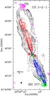 |
Fig. 1 Emission of the Cep E-mm outflow as observed in the CO 2–1 line with the PdBI at 1″ resolution by Lefloch et al. (2015). Four main velocity components are detected: a) the outflow cavity walls (black) emitting at low velocities, in the range [−8;−3] km s−1 and [−19;−14] km s−1 in the northern and southern lobe, respectively; b) the jet, emitting at high velocities in the range [−135;−110] km s−1 in the southern lobe (blue) and in the range [+40;+80] km s−1 in the northern lobe (red); c) the southern terminal bow shock HH377, integrated in the range [−77,−64] km s−1 (green); and d) the northern terminal bullet NB integrated in the velocity range [+84,+97] km s−1 (magenta). First contour and contour interval are 20% and 10% of the peak intensity in each component, respectively. The synthesized beam (1.″07 × 0.″87, HPBW) is shown in the bottom left corner. The dashed black box encloses the central protostellar region studied with the SO NJ = 54–43 line (see Fig. 2). The main axes of the northern and southern lobes of the jet are shown with black arrows. |
3 Observations
3.1 SO NJ = 54–43
The NOEMA array was used in configuration A with eight antennas on 23 and 30 December 2016 to observe the spectral band 204.0–207.6 GHz toward the Cep E-mm protostellar system as part of the Large Program Seeds Of Life In Space (SOLIS; Ceccarelli et al. 2017). The field of view of the interferometer was centered at position α(J2000) = 23h03m13s.00 δ(J2000) = +61°42′21.″00. The wideband receiver WIDEX covered the spectral band 204.0–207.6 GHz with a spectral resolution of 1.95 MHz (≃2.8 km s−1), which includes the rotational transition SO NJ = 54–43 at 206176.005 MHz. The spectroscopic parameters of the transition were taken from CDMS1 (Müller et al. 2005). The precipitable water vapor (PWV) varied between 1 mm and 2 mm (between 2 mm and 4 mm in the second night) during the observations. Standard interferometric calibrations were performed during the observations: J2223+628 was used for both amplitude and phase calibration. Bandpass calibration was performed on 3C454.3. Calibration and imaging were performed by following the standard procedures with GILDAS-CLIC-MAPPING2. The emission of the SO NJ = 54–43 line was imaged using natural weighting, with a synthesized beam of 0.52″ × 0.41″ and a position angle PA of 359° (see Table 1). Self-calibration was applied to the data. The shortest and longest baselines were 72 m and 760 m, respectively, allowing us to recover emission at scales up to 12″. The primary beam of the interferometer (≈24.4″) allowed us to recover emission up to ~12″ (104 au) away from protostars Cep E-Aand Cep E-B, while the synthesized beam gave access to spatial scales of ~400 au.
In order to estimate the fraction of the IRAM 30m flux collected by NOEMA, we compared the SO NJ = 54–43 molecular spectrum of the ASAI millimeter line survey of the Cep E-mm protostellar core from Ospina-Zamudio et al. (2018) and the NOEMA spectrum degraded at the same angular resolution. We found that about 34% of the IRAM 30 m flux was recovered by the interferometer.
Properties of the observational dataset.
3.2 CO 2–1
We made use of the CO J = 2–1 data obtained at a spatial resolution of ~1″ with the IRAM Plateau de Bure Interferometer (PdBI). The observation procedure and the data were presented in Lefloch et al. (2015). In order to map the molecular emission along the outflow, the 1.3mm band was observed over a mosaic of seven fields centered at the offset positions (−9.0″, −20.8″), (−4.5″, −10.4″), (+0″, +0″), (+4.5″, +10.4″), (+4.5″, +20.8″) with respect to Cep E-A.
As explained by the authors, the emission at scales larger than 10″ was recovered by combining the PdBI data with the synthetic visibilities derived from an IRAM 30 m map of the region. The jet total flux was recovered by the interferometer in both lobes (Lefloch et al. 2015). The intensities were converted from Jy beam−1 into K using a conversion factor of 26.88.
4 Jet-envelope interaction
4.1 Molecular gas distribution
The CO and SO emissions from the high-velocity jet in the protostellar region around Cep E-A are displayed in Fig. 2. The line fluxes were integrated in the velocity range [+40;+80] km s−1 and [−110;−50] km s−1 in the northern and southern lobe, respectively. We observe a very good morphological match between the SO and CO emission distributions at close distance (<2″) from the protostar. Both species trace a strongly collimated jet with a diameter ≤0.4″ (~320 au), unresolved in our observations. At a larger distance (>2″) from protostar A, the CO emission gradually broadens until it reaches a diameter of about 2″ (FWHM), while the SO emission is mainly unaffected. Comparison of CO position-velocity diagrams across the jet main axis in Fig. 3 confirms that the high-velocity emission (V = 60 km s−1) is unresolved near the protostar (offset δ = 0″), while it reaches a diameter of 2″ at δ > 1.5″.
Hence, these observations draw the picture of a two-component jet: a central, highly collimated component of diameter <320 au, specifically probed by SO, surrounded by a radially extended gas layer detected in CO. The pattern revealed in our observations is consistent with the pattern recently reported by Podio et al. (2021) in the CALYPSO sample of young low-mass protostellar outflows.
The situation is more complicated in the southern lobe by the high-velocity jet powered by protostar B, which propagates in the east-west direction at 1″ south of protostar A (Ospina-Zamudio et al. 2018). A signature of the B jet is detected as a redshifted clump near 23h03m13s.0 +61°42′25″ (Fig. 2). We note that the southern (blueshifted) lobe of the A jet displays a highly collimated SO emission, with a diameter similar to that of the northern lobe.
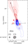 |
Fig. 2 Distribution of the CO 2–1 and SO NJ = 54–43 velocity-integrated emission in the central protostellar region. Northern lobe (red): emission is integrated in the velocity range [+40;+80] km s−1 and is displayed in thin and thick contours for CO and SO, respectively. Southern lobe (blue): emission is integrated in the velocity range [−110;−50] km s−1 and is displayed in thin and thick contours for CO and SO, respectively. The velocity interval was chosen in order to include the region of jet acceleration close to the protostar (see Sect. 4.2). The beam sizes (HPBW) of the CO and SO observations (1.07″ × 0.87″ and 0.52″ × 0.41″, respectively) are shown with ellipses in the bottom left corner. The velocity resolution of the CO (SO) observations is 3.3 km s−1 (2.8 km s−1). The first contour and contour interval are 20% and 10% of the peak intensity in each component. The arrow draws the main axis of the jet from protostar B (from Ospina-Zamudio etal. 2018). |
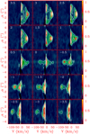 |
Fig. 3 Position-velocity diagram of the CO 2–1 line emission across the jet main axis (see Fig. 1). The beam size (HPBW) of the CO observations is 1.07″ × 0.87″. The velocity resolution of the observations is 3.3 km s−1. The relative distance to the protostar δ (in arcsecond) is indicated in the top left corner. The first contour and contour interval are 10% and 15% of the peak flux, respectively. Fluxes are expressed in Jy beam−1. |
4.2 Jet acceleration
The orientation of the main axis of the jet at large scale was determined from the distribution of the high-velocity CO emission integrated in the intervals [+40; +80] km s−1 and [−135; −110] km s−1 in the northern and southern lobe, respectively (see Fig. 1). The former is found to make a position angle (PA) of +20°, while the latter makes a PA of +204°. These values based on the large-scale CO distribution are somewhat indicative because of the complexity of the outflow kinematics and the evidence of changes in the direction of propagation along the outflow, as illustrated at large scale by the difference of orientation of the two northern outflow cavities (Fig. 1). This point is discussed in Sect. 6.
The distribution of the CO emission as a function of velocity along the main jet axis is displayed in Fig. 4. The emission is dominated by the protostellar source Cep E-A at Vlsr = −10.9 km s−1. At large distance from the source (|δ| > 10″), the jet radial velocity V reaches a steady value of ~+65 km s−1 and −125 km s−1 in the northern and southern lobe, respectively.
However, in the inner 5″ (~4000 au) around the protostar, the CO jet displays much lower velocities than the asymptotic values measured at large distances. More precisely, the velocity gradually increases from ambient at Vlsr = −10.9 km s−1 to the terminal value on a scale of a few arcseconds. The radial velocity profile V as a function of distance δ to the protostar along the jet main axis can be fit by the simple relation

where V0 is the jet asymptotic radial velocity relative to the protostar, and δ0 is the length scale of the jet acceleration process.
The length scale δ0 and the jet velocity V0 (relative to Cep E-A) were determined from a best-fitting procedure to the CO position-velocity diagram. The procedure yields δ0 = 693 au (590 au) and a jet velocity V0 = +75 km s−1 (−118 km s−1) in the northern (southern) jet. The agreement between the best-fitting V0 values and the observational determination of the jet velocity relative to the source is very good (+76 km s−1 and −114 km s−1 for the northern and southern lobes, respectively; see Sect. 2 and Fig. 4) and supports our simple modeling. The close agreement between the two values of δ0 suggests that the physical conditions are similar at subarcsecond scale around Cep E-A.
Intriguingly, the jet appears to be accelerated on a scale of 700 au and exceeds the size of the protostellar disk and hot corino of Cep E-A ~200 au by far (Lefloch et al., in prep.). Inspection of the CO and SO position-velocity diagrams along the major axis of the jet in the central protostellar regions reveals a more complex situation, as shown in the middle and bottom panels of Fig. 4. The CO emission distribution reveals that a small fraction of material is accelerated at velocities up to ~60 km s−1 at a few 100 au from protostar A, which is similar to the jet terminal velocity.
The SO NJ = 54–43 emission distribution obtained at 0.4″ resolution, a factor of 2 higher than in the CO observations, brings more insight into the gas acceleration, as shown in Fig. 4 (bottom panel). The bulk of the SO emission arises from three compact knots: N0a, located at less than 0.2″ (~160 au) from Cep E-A, with velocity V = +54.6 km s−1, and N0b and N0, detected in the northern jet at δ = +2″, V = +39.8 km s−1 and δ = +3.1″, V = +44.5 km s−1, respectively. Figure 2 shows that the SO emission in the velocity range of these three knots ([+40; +80] km s−1) is unambiguously located in the northern lobe of the Cep E-A jet. As shown by Ospina-Zamudio et al. (2018), the second high-velocity collimated jet powered by the secondary companion Cep E-B propagates in the east-west direction about 1″ south of Cep E-A (see their Fig. 2), nearby enough to raise the question of a possible contamination in the distribution of the molecular gas emission.
However, the spatial distribution of the SO emission at 0.4″ resolution integrated between +40 and +80 km s−1 (Fig. 2) shows that all three knots are associated with the Cep E-A northern jet. Interestingly, the bulk velocity of the SO gas appears to vary monotonically between these knots.
To summarize, the analysis of the jet kinematics reveals two components: a component with an extremely high velocity that is highly collimated and originates from the protostar, detected in SO and CO, and a secondary, more extended layer of accelerated gas detected mainly in CO.
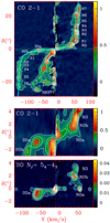 |
Fig. 4 Position–velocity diagrams of the CO and SO emission along the jet main axis (see Fig. 1). Top: CO 2–1 as observed at 1″ with the IRAM interferometer. The different knots identified close to the protostar are indicated. The best-fitting relation to the gas acceleration |V – Vlsr|/V0 = exp(−δ0/δ) is superimposed in cyan. Middle: Magnified view of the CO 2–1 emission in the central protostellar region near Cep E-A. Bottom: SO NJ = 54–43 as observed at 0.4″ resolution with NOEMA. The first contour and the contour interval are 10% and 15% of the peak intensity, respectively. The dashed red lines mark the ambient cloud velocity (Vlsr = −10.9 km s−1). The velocity resolution of the CO and SO observations is 3.3 km s−1 and 2.8 km s−1, respectively. Fluxes are expressed in Jy beam−1. |
4.3 Envelope entrainment
4.3.1 Northern lobe
Inspection of the CO position-velocity diagrams across the jet main axis (Fig. 3) shows that the ambient gas emission extends up to distances of ±4″ from the jet (see, e.g., panel δ = +2″). The CO jet is well identified at V ≃ +65 km s−1. In the close environment of the protostar at δ = 0″, the velocity distribution between the outer quiescent regions of the envelope and the jet is continuous, as shown in Figs. 3–4. This means that the ambient quiescent protostellar material from the envelope is dragged away and accelerated by the jet. The CO emission of this entrained component is brighter than the jet material launched from the protostar and its associated knots, hence suggesting an accelerated jet. The gas entrainment is best seen in the PV diagrams δ = + 0″ to δ = + 1.5″ across the jet main axis (see the top panels in Fig. 3). At larger distances from the protostar, δ ≥ 2.0″, the jet signature (V = +65 km s−1) gradually separates from the entrained gas emission. This suggests that the entrainment process loses its efficiency as the distance from the protostar increases beyond ~2− (1600 au).
4.3.2 Southern lobe
The evidence of jet-entrained gas near Cep E-A at δ = 0.0 is much weaker. The emission in the range [−70;−11] km s−1 appears to be collimated with a typical diameter of 1.5″, consistent with the value measured in the northern jet in the range [+40;+60] km s−1. The main difference with the northern lobe is that there is no jet entrainment of material at distance > 1″ (800 au), that is, that there is far less jet-entrained material in the southern lobe. The CO jet emissivity is inhomogeneous and displays a maximum between δ = −1″ and δ = −3″ (see Fig. 3). This maximum coincides with the region of propagation of the Cep E-B jet, as mapped in the SiO 5–4 line by Ospina-Zamudio et al. (2019). We speculate that the absence of gas entrainment in the southern lobe could result from the interaction between the two outflows-jets.
As discussed by Lefloch et al. (2015), a detailed analysis of the momentum budget in the outflow southern lobe showed that the high-velocity jet carries away the same amount of momentum as the low-velocity gas (1.7 versus 2.6 M⊙ km s−1, respectively). This led the authors to conclude that the low-velocity outflow is driven by the protostellar jet itself. This result is supported by the distribution of the CO emission in the position-velocity diagram along the main jet axis. The top panel of Fig. 4 shows that the low-velocity gas appears to be gradually accelerated from the protostar up to the terminal shock HH377 following a Hubble law relation: (V – Vlsr) ∝ δ, where δ is the angular distance to the protostar. This kinematical feature is an unambiguous signature of a jet bowshock-driven outflow (Raga & Cabrit 1993; Wilkin 1996; Cabrit et al. 1997).
5 Mass ejection
Bright knots of CO gas in the molecular jet were first reported by Lefloch et al. (2015). In this section, we present a detailed study of the knots and show that a simple ballistic modeling can account for their dynamical properties.
5.1 Kinematics
We have searched for knots along the jet in both the northern and the southern lobes from the CO jet intensity map in Fig. 1 and the CO position-velocity diagram along the jet main axis (Fig. 4). We identified ten (eight) CO knots in the northern (southern) lobe, labeled N0a to N7 (S0a to S6) (see Table 2).
The SO 54–43 observations provide a more concentrated view of the knots located at a few arcseconds from the protostar. In the northern jet, we detect knot N0a at δ = +0.2″ and V = +54.6 km s−1 and knot N0b at δ = +2.0″ and V = +39.8 km s−1 (see the bottom panel in Fig. 4). In the southern jet, we detect a knot, referred to as S0a, near the offset position δ = −0.8″ (and V = −62.5 km s−1). We note that the SO emission looks elongated along the jet axis and it is hence unclear whether more than one knot is present. The emission from the southern jet close to Cep E-A does not display the same fragmented structure as in the north. The similarity in the ejection velocities of S0a and N0a, both at short distance from Cep E-A, suggests that they are associated with the same ejection event and that the physical conditions of jet acceleration are comparable in both lobes.
We derived the main physical properties of the identified knots: coordinates, size (beam-deconvolved), distance d from the protostar, radial velocity V, dynamical age tdyn = d/V × tan i, and mass. The positions and sizes of the different knots were determined from a 2D Gaussian fit to the CO flux distribution, except for knots N0a-N0b, whose parameters were determined from SO. The velocities were measured in the CO position-velocity diagram in Fig. 4. These parameters are summarized in Table 2. For the sake of completeness, we included the parameters of the terminal shocks NB and HH377 (see Fig. 1).
The knot dynamical ages appear to span the time range 60–1500 yr. Interestingly, HH377 and NB have comparable dynamical ages, so that the two series of knots in the northern and southern appear to cover the same time interval of mass-ejection events.
Figure 5 displays the distribution of knot velocities relative to Cep E-A as a function of the distance to the protostar. We superimposed the best-fitting solutions to the CO position-velocity diagrams in blue and red for the southern and northern lobes, respectively. We adopted an uncertainty of +0.5″ in position (one beam size) and a value of +5 km s−1 in velocity (mean knot line width) (see Table 2). It immediately follows that all the knots but N0a trace the overall CO gas distribution in the jet. The amplitude of the velocity fluctuations with respect to the bulk of jet material velocity is weak, on the order of a few km s−1.
Knots are not regularly distributed along the jet at equal distances one from the other. At large distance from the protostar, typically 10″, the separation between knots tends to increase from ~2.5″ to ~4.5″ in the southern lobe (see Fig. 5). The knot distribution is more complex in the northern lobe, but their separations are on the same order, ~2.5″ (2000 au) and 4.5″ (3700 au) for close (e.g., N2/N3) and remote (N1/N2) knots, respectively. This distribution may be biased by the gas acceleration in the central protostellar regions. For this reason, in order to obtain more insight into the knot distribution, we computed the distribution of time intervals between subsequent knots as a function of distance to the protostar. This is displayed in Fig. 6. A marked separation is observed in the southern lobe (in blue) between the knots located at ≤10–13″ from the protostar, with a short ∆tdyn~50–80 yr, and the more distant knots, with ∆tdyn ~150–200 yr. A similar pattern is observed in the northern lobe (red), with similar time intervals close to and far away from the protostar. We consider the case of knots N2/N3 at 9–11″ as peculiar; we suspect that this anomaly is caused by the interaction of the knots with the ambient gas.
To summarize, the analysis of the knot interval distribution suggests the presence of two timescales: a short time interval ∆t ~ 50–80 yr close (≤12″) to the protostar, and a longer timescale ∆t ~ 150–200 yr at larger distances from the protostar. This knot interval distribution could be explained as due to a periodic process that takes place at the base of the Cep E-mm jet. We examine this hypothesis in more detail in the next section.
Knot identification and properties.
 |
Fig. 5 Distribution of knot velocity peaks along the main jet axis as a function of distance δ to Cep E-A in the northern (red) and southern (blue) jet components. The best fit to the northern (southern) jet velocity relative to the source (V – Vlsr)/V0 = exp(−δ0/δ) with δ0 = 693 au (δ0= 590 au) and V0 = +75 km s−1 (V0 = −118 km s−1) is drawn by the solid curve. |
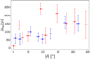 |
Fig. 6 Distribution of time intervals between subsequent knots as a function of distance to the protostar along the jet main axis in the northern (red) and southern (blue) lobes. |
5.2 Knot mass distribution
We have determined the mean gas column density of the knots from a radiative transfer analysis of the CO 2–1 line emission, using the code MadeX (Cernicharo 2012) in the large velocity gradient approximation and the CO-H2 collisional coefficients from Yang et al. (2010). In this simple model, we assumed that the CO emission measured toward the knots arises from a single physical component. In other words, the contributions of the entrained gas envelope and the inner jet material along the line of sight, both discussed in Sect. 4.3, were neglected with respect to that of the knots. Line widths and intensities were obtained from a Gaussian fit to the line profiles at the flux peak of the knot (see Table 2). The peak intensity of the knot was sometimes found to lie off the jet main axis by a fraction of a beam. This indirectly reveals a complex knot structure at subarcsecond scale, with some small velocity shifts between the intensity peak and the jet main axis. We adopted the jet H2 density and temperature derived by Lefloch et al. (2015) and Ospina-Zamudio et al. (2019) in the southern and northern lobes from a CO multitransition analysis. The total H2 mass and column density were subsequently obtained from N(CO) adopting a standard CO to H2 relative abundance ratio of 10−4.
We derived knot masses of the order of 10−3 M⊙ (see Table 2). The knots are more massive in the north than in the south by a factor of a few. In both lobes, the masses of the knots tend to increase beyond 10″ (8000 au), a distance corresponding to knots N3 and S4 in the northern and southern lobe, respectively, or, equivalently, to a dynamical timescale of 500 yr. As discussed in Sect. 4.3, the CO position-velocity diagrams show evidence of protostellar material entrainment by the northern jet only in the central 2″–3″ close to Cep E-A; therefore, it seems unlikely that the observed knot mass increase is related to the jet-envelope interaction. This point is addressed in more detail in the following section, in which we consider the possibility of dynamical interactions of the knots.
The mass of knot NB (1.3 × 10⁻³ M⊙) is similar to that of the other knots, in agreement with the interpretation that NB is the jet terminal bow shock. Our estimate of the HH377 mass was found to agree well with the previous estimate obtained by Lefloch et al. (2015) (≃6 × 10⁻³ M≃), based on a detailed CO multiline analysis. In other words, the mass of HH377 amounts to that of four to five knots, consistent with the number of undetected knots in the southern lobe. The derived value must be considered a lower limit as the CO abundance could be lower if dissociative J-type shock components were present (see Gusdorf et al. 2017).
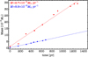 |
Fig. 7 Cumulative knot mass function in the northern (red) and southern (blue) lobes. Knot NB (S6) and its associated dynamical timescale is taken as reference in the northern (southern) lobe. The best linear fits are drawn by dashed lines. |
5.3 Mass-loss rate
The determination of knot masses and their dynamical timescales allows us to retrieve the mass-loss history of Cep E-A and its variations. We report in Fig. 7 the cumulative mass of ejected knots as a function of time. In this analysis, the origin of the time axis t = 0 is defined by the knots NB and S6 in the northern and southern lobes, respectively (strictly speaking, HH377 is not a simple knot, as discussed in the next section). Then, the cumulative mass is obtained by summing one after the other the mass of the subsequently ejected knots; the corresponding time is simply obtained from the distribution of knot dynamical timescales, starting again from the most distant ones (NB/S6). We note that the reference time t = 0 in Fig. 7 differs between outflow lobes as the reference knots NB and S6 taken as reference to compute the cumulative mass function have different dynamical ages.
Figure 7 shows that the cumulative mass function is well fit by a linear function of slope  in the southern lobe (dashed blue line) and
  in the northern lobe (dashed red line), respectively. We can draw two conclusions from this figure.
First, the mass-loss rate appears steady over the whole knot ejection process in both lobes. We note that the possibility of knot interactions along the jet, as discussed in Sect. 5.4, should not affect the slope of the cumulative mass function, but only the mass of specific ejecta.
Second, the mass-loss rate appears to be higher in the northern lobe by about a factor 3. The main difference between both lobes lies in the fact that northern knots are entraining and accelerating a layer of protostellar material. This phenomenon is not detected in the southern lobe (see Sect. 4.3). It naturally explains the higher amount of high-velocity material in the northern lobe and the difference in the mass-loss rates observed between both lobes. The scatter of the knot mass distribution is also larger, and we propose that it might result from the jet interaction with the ambient medium.
5.4 Ballistic modeling
The observed variability of the separation between knots, as discussed in Sect. 5.1, has usually been interpreted as the result of the superposition of several ejection modes with different periodicity (Raga et al. 2012), related to velocity or density variations in the ejection process. Here, we propose that the minimum time interval between two consecutive knots corresponds to the period of the variable ejection process and that the radial velocity fluctuations reported in Table 2 result from this variability. Then, the apparent bimodal distribution of knot separation can simply be accounted for by dynamical interactions in the nearby environment of protostar A.
From the knot dynamical ages (see Table 2), we estimate a period τej = 55 yr for the ejection process. It is then possible to translate the knot dynamical age into the number of elapsed periods since its formation, so that each knot can be uniquely identified from its associated period number n. This is represented in Fig. 8, where the ages of the individual knots are plotted as a function of the number n of periods of the ejection process. The typical uncertainty on the knot location corresponds to ~1″ the synthetic beam size (HPFW) of the CO observations, which results in an uncertainty ∆n ~ 1 on the period number n.
Inspection of the knot dynamical ages shows that some events in the northern jet exhibit a counterpart in the southern jet, suggesting that they are associated with the same mass-loss event. This is the case, for example, of knots N0/S1 (n = 4), N1/S2 (n = 5) and N3/S5 (n = 11). As discussed in Sect. 5.1, the knots with low n values (n < 10), which are observed at close distance from the protostar, tend to be associated with subsequent ejections, while knots with large period numbers appear to be unevenly distributed (see Fig. 8).
The bottom panel in Fig. 4 shows that the young knots N0a-N0b-N0 are ejected with marked velocity variations. The youngest knot N0a moves at a velocity that is 15 km s−1 faster than N0b, while they are separated by 1500 au (~1.8″). Hence, it should take about 500 yr for N0a to catch up and collide with N0b. The collision is bound to occur at the typical distance of 6500 au, that is, 8″ from the protostar. This collision timescale corresponds to a period number n ≃ 11. As discussed above (see also Fig. 8), this value of n is the threshold beyond which the knot distribution no longer displays evidence of subsequent ejections. We also note that on average, the mass of the knots is higher for dynamical timescales longer than 500 yr. We conclude that the bimodal knot distribution observed in the jet is most likely the result of collisions between subsequent knots ejected with markedly different velocities.
We speculate that the elongated appearance of knot S0a might trace the interaction of two subsequent ejections. The spatial structure of knots is out of reach at the angular resolution of the CO data. Observations at higher angular and spectral resolutions are required in order to fully resolve the structure of the knots and to search for the reverse shocks that are expected to form between colliding mass ejecta.
Ayala et al. (2000) proposed that HH377 traces the impact of the southern jet in a dense molecular gas clump, explaining that HH377 propagates at a velocity V ≃ −67 km s−1, strongly reduced with respect to the jet velocity itself (−125 km s−1). We propose that the southern knots, after they reached the terminal jet velocity V ≃ −125 km s−1, propagate along the jet until they finally impact the terminal bow shock. In the impact, their velocity suddenly drops, while their material feeds the HH object. The distance between S6 and HH377 is ~4″ (3300 au), so that it takes about 270 yr for a knot to cover this distance, which is far shorter than the duration of the mass-loss phase, as estimated from the dynamical age of the oldest northern knots (~1500 yr; see Fig. 8).
The mass of HH377 is ~6 × 10⁻³ M⊙, which amounts to the mass of ~6 knots (adopting an average knot mass of 10−3 M⊙). This number agrees reasonably well with the lack of knots in the range n = 17–26 in the southern lobe, whereas four knots are detected in the northern jet. According to our mass-loss rate analysis, the HH377 mass corresponds to the amount of jetmaterial ejected for ~670 yr. This would imply a dynamical age of ~1410 yr for the southern jet, which agrees very well with the dynamical age of knot NB (1440 yr; Table 2), at the tip of the northern jet.
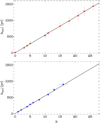 |
Fig. 8 Distribution of knot dynamical ages as a function of the number of periods of the periodic mass-ejection mechanism n in the northern (upper panel) and southern (lower panel) lobes. |
6 Jet wiggling
As recalled in Sect. 1, the cause of the wiggling structure observed in molecular outflows is not completely understood. Several models have been proposed to account for the variability of the ejection direction: orbital motion of a binary system (Masciadri & Raga 2002), jet precession due to tidal interactions between the associated protostellar disk and a noncoplanar binary companion (Terquem et al. 1999), misalignment between the disk rotation axis, and the ejection mechanism (Frank et al. 2014). The latter model requires only a single protostar.
The limited angular resolution of our observations (320–800 au) does not allow us to probe the disk scale or the jet launch region. Here, we consider the two following classes of periodic mass-ejection models proposed to account for the wiggling pattern of protostellar outflows: (i) jet precession and (ii) orbital motion around a binary companion. Both models produce a garden-hose effect (Raga et al. 1993): close to the source, the jet propagates almost parallel to the main jet axis, while further downstream, the side-to-side wiggling is amplified as the fluid parcels ejected in different directions diverge from each other. Outflow morphology allows distinguishing between the two models: an antisymmetric S shape is observed in the precession scenario, while a mirror-symmetric W shape is observed in the orbital motion scenario (e.g., Raga et al. 1993; Masciadri & Raga 2002; Noriega-Crespo et al. 2011; Velazquez et al. 2013; Hara et al. 2021).
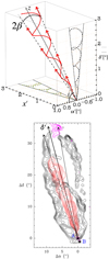 |
Fig. 9 Jet precession in Cep E. Top: wiggling model. The jet precession axis is represented by the continuous gray line. The jet moves over a cone of half-opening angle β It makes an inclination angle i with respect to the plane of the sky (α′,δ′). The locus of the ejection direction is drawn by the red curve. In the plane of the sky (α′,δ′), the projection of the locus is represented by the black line. Bottom: projected view of the jet axis associated with the current high-velocity emission, the previous ejection associated with knot NB, and the precession axis δ′, superimposed on the CO 2–1 outflow emission (see Fig. 1). |
6.1 Precession
We adopted a more detailed modeling of the jet precession than the previous works by Eisloeffel et al. (1996) and Noriega-Crespo et al. (2014) by making use of the spatial distribution of knots to constrain the dynamical parameters of the ejection process, under the assumption of ballistic motion. We considered a jet precessing inside a cone of main axis z and half-opening angle β (see the top panel of Fig. 9). The jet produces a spiral pattern described by the following parametric equations (Raga et al. 1993):
 (1)
(1)
and
 (2)
(2)
where λ is the spatial period and ϕ is the phase angle. In general, the precession axis makes an inclination angle i with respect to the plane of the sky, and the projected coordinates (α′,δ′) in this plane are given by
 (3)
(3)
We adopted for Cep E an inclination angle i = 47°, as mentioned in Sect. 2. We first determined the parallactic angle of the jet precession axis z in the plane of the sky from the average position angle of the lines formed by the source and the knots, including NB and HH377. Proceeding independently for the northern and southern lobes, we find a misalignment of about 7° between the two axes. The configuration in the northern outflow is summarized in the bottom panel of Fig. 9: the loci of the current jet, the precession axis δ′, and the direction of the previous ejection associated with knot NB.
After determining the orientation of the jet precession axis z, we computed the coordinates (α′,δ′) of each knot in the plane of the sky. They are reported in Fig. 10. The northern (red) knots show an increasing deviation in the positive α′ direction until δ′ = 26″. Farther away, NB is detected at negative offsets α′ = −3″ from the precession axis. In the southern lobe, (blue) knots appear to lie along the precession axis, with small positive offsets at less than 8000 au from the protostar. The spatial distribution of the knot displayed in Fig. 10 around the driving protostar at δ = 0″ is consistent with an S-shape symmetry. A W-shape symmetry would require a knot distribution with negative offsets in the southern lobe, which is not compatible with the observational data. We conclude that comparison of the northern and southern knot spatial distributions unambiguously favors an S-shape geometry.
Using Eqs. (1)–(3), we then searched for the parameter set (λ, β, ϕ) that best reproduces the location of the knots in the plane of the sky. We modeled the northern and southern lobes separately. From the total jet velocity Vt, we derived the precession period τp = λ/Vt. The best-fitting model was obtained through a least-squares method and is drawn as a (red/blue) continuous curve in Fig. 10. The parameters of the best-fitting model are presented in Table 3.
Our model succeeds in reproducing the spatial distributions of the knots both in the northern and the southern jet. In the latter case, we note, however, that the variations in the knot distribution are smaller than the position uncertainties, hence enlarging uncertainties in the parameters of the best-fitting solution (see Table 3). The values of the phase angle ϕ and the precession period τP are found to be similar between the northern and southern lobes. This is consistent with symmetric ejections, in agreement with the observational data.
Table 3 shows that differences are observed between the northern and southern lobes in the alignment of the precession axes, the jet velocities, and the half-opening precession angle. We propose that this is related to the different environmental conditions between the outflow lobes (Hirth et al. 1994; Velázquez et al. 2014).
Precession changes the direction of the jet propagation with respect to the plane of the sky, and therefore affects the knot radial velocity. Taking into account the inclination of the Cep E jet with respect to the plane of the sky, the half-opening angle of its precession cone can yield velocity variations up to 15 km s−1. Hence, the combined effect of the ejection variability and precession is expected to generate velocity variations of 25 km s−1 or more, which could explain the higher radial velocity reported for NB. To conclude, velocity variations as large as those measured between NB and younger knots are consistent with the wiggling dynamics of the Cep E jet; variations like this are expected to be rare as the jet dynamical age is similar to the precession period.
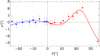 |
Fig. 10 Positions of the CO knots with respect to the precession axis in the northern (red) and southern (blue) lobe. The solid line draws the best-fitting precession model to the observational data. |
Parameters of the jet precession model.
6.2 Origin of the jet wiggling
Masciadri & Raga (2002) first proposed that the orbital motion of a binary system could account for the wiggling morphology of outflows. The authors found that the same description of a precessing jet model could be applied at a distance from the precession axis larger than the binary separation r0. In this case, the half-opening angle is determined by the ratio of the orbital velocity and the total jet velocity tan β = Vo/Vt. Moreover, the authors related the distance ∆z between a maximum and a minimum in y (∆z ~ 23″ for Cep E) to the separation r0 of the two binary components,
 (4)
(4)
which implies r0 ~ 140 au and an orbital period τo of
 (5)
(5)
at the distance of Cep E-mm (819 pc). Then, we estimate a typical mass
 (6)
(6)
for the components of the binary. In their original work, Masciadri&Raga(2002) derived this relation under the assumption of equal-mass components. This value is too high to be reconciled with the luminosity of the protostellar core (100 L⊙) and the core masses derived from the dust thermal emission at arcsecond scale by Ospina-Zamudio et al. (2018). Applying Eq. (6) to protostar B, which lies at a distance of 1.2″ (~9000 au) from A and assuming the same orbital period, the mass required would be even higher than ~20 M⊙.
As discussed in the previous section, the spatial distribution of the knot along the jet (Fig. 10) appears to agree better with an S-shape than with a W-shape symmetry. The symmetry of the distribution therefore supports jet precession rather than an orbital motion scenario as the origin of the change in outflow direction in Cep E.
To summarize, the orbital motion scenario fails to account for the properties of the spatial distribution of the knot in the Cep E protostellar jet. Our analysis favors a jet precession scenario as origin of the outflow wiggles. As mentioned above in this section, Terquem et al. (1999) proposed that jet precession originates in the tidal interaction between the protostellar disk driving the jet and a noncoplanar binary companion. The authors applied their analytic model to the case of Cep E based on the parameters estimated by Eisloeffel et al. (1996). They concluded that the system is a very close binary with a distance in the range 4–20 au and a small disk radius R = 1–10 au. Taking into account the much longer precession timescale implied by our new model, 2000 yr instead of 400 yr, the separation of the binary increases by a factor ~2 up to 8–40 au (0.″01–0.″05), but unfortunately, the linear scales involved remain beyond the reach of the NOEMA interferometer. We note that also in the scenario proposed by Terquem et al. (1999), protostar B cannot be responsible for the precession observed in the jet from protostar A.
7 Conclusions
We have carried out a detailed kinematical study of the high-velocity jet of the intermediate-mass class 0 protostar Cep E-A using observations from the IRAM interferometer at (sub)arcsecond resolution in the CO 2–1 and SO NJ = 54–43 lines. Our conclusions are listed below.
The CO high-velocity jet consists of two components: a central component with a diameter of ≤400 au associated with high-velocity molecular knots (also detected in SO), and a surrounding gas layer accelerated on a length scale δ0 ~700 au, whose diameter gradually increases up to several 1000 au at about 2000 au from the protostar.
Along the main jet axis, the CO gas velocity can be simply fitted as a function of distance δ to the protostar by the relation (Vr − Vlsr)/V0 = exp(−δ0/δ), where Vlsr = −10.9 km s−1 is the ambient cloud velocity, V0 is the terminal velocity in the jet lobe relative to the source ~+75 km s−1 (−118 km s−1), and δ0 is the length scale ~700 au (600 au) in the northern (southern) hemisphere. Analysis of the CO position-velocity diagrams shows that the jet layer consists of quiescent protostellar material entrained by extremely high velocity knots. The material entrainment appears to be more efficient in the northern than in the southern lobe.
The jet molecular gas emission reveals 18 bright knots in either lobes of the jet with a dynamical timescale of 55 yr between subsequent ejections close (<1000 au) to the protostar. The knots have a typical size of 2″, with a tendency to increase with distance to the protostar. We have identified knots NB and HH377 as the terminal bow shocks of the northern and southern lobes, respectively.
Assuming a standard CO abundance of 10−4 relative to H2, a simple radiative transfer analysis in the LVG approximation with MadeX yields a typical mass of 10−3 M⊙ for the bullets. SO observations at 0.4″ show that the knots leave the inner protostellar regions (~200 au) at high velocity, with marked velocity fluctuations between subsequent ejections. The cumulative knot mass function allows us to estimate mass-loss rates of 2.7 × 10⁻⁵ M⊙ yr−1 and 8.9 × 10⁻⁶ M⊙ yr−1 in the northern and southern lobes, respectively. The jet mass-loss rates appear steady with time. The higher mass-loss rate in the north is consistent with protostellar material entrainment by the jet.
The knot interval distribution between subsequent knots is approximately bimodal with intervals of ~55 yr and ~150 at short (<12″) and large (>12″) distance from the protostar. In the northern jet, the velocity fluctuations are large enough (~15 km s−1) that the spatial separation between knots can be overcome in a dynamical timescale of ≃500 yr, when knots will have traveled a typical distance of 12″ (104 au) from the protostar. This naturally explains the lack of knots at large distances from the source. This result is also supported by the higher masses found for the knots at larger distances.
Analysis of the knot spatial distribution suggests precession as the origin of the wiggling structure of the outflow. Applying the Masciadri-Raga formalism, we obtained an accurate description of the jet morphology, taking into account the outflow inclination angle with respect to the plane of the sky. The same model allowed us to discard binary orbital motions as the source of the Cep E-mm jet wiggling, since it would require protostellar masses too high to be reconciled with the source luminosity and mass. We propose that jet precession originates in tidal perturbations of the associated protostellar disk by a binary companion, yet to be identified, in agreement with previous work by Terquem et al. (1999).
The results discussed throughout this article not just present the kinematic information about the Cep E outflow-jet system the but also allow us to have a closer understanding on the processes involved in the jet formation and interaction of its surroundings. In fact, this study contributes for a better comprehension of the difference between low-and high-mass star formation feedback processes.
Acknowledgements
Based on observations carried out with the IRAM NOEMA interferometer. IRAM is supported by INSU/CNRS (France), MPG (Germany) and IGN (Spain). AS, BL, PR-RO, acknowledge support from the European Union’s Horizon 2020 research and innovation program under the Marie Skłodowska-Curie grant agreement No 811312 for the project “Astro-Chemical Origins” (ACO) and the European Research Council (ERC) under the European Union’s Horizon 2020 research and innovation program for the Project “The Dawn of Organic Chemistry” (DOC) grant agreement No 741002. DSC is supported by an NSF Astronomy and Astrophysics Postdoctoral Fellowship under award AST-2102405. A.V. and A.P. are the members of the Max Planck Partner Group at the Ural Federal University. A.P. and A.V. acknowledge the support of the Russian Ministry of Science and Education via the State Assignment Contract no. FEUZ-2020-0038.
References
- Ayala, S., Noriega-Crespo, A., Garnavich, P. M., et al. 2000, AJ, 120, 909 [NASA ADS] [CrossRef] [Google Scholar]
- Bachiller, R. 1996, ARA&A, 34, 111 [NASA ADS] [CrossRef] [Google Scholar]
- Bally J. 2016, ARA&A, 54, 491 [NASA ADS] [CrossRef] [Google Scholar]
- Cabrit, S., Raga, A., & Gueth, F. 1997, in Herbig–Haro Flows and the Birth of Stars; IAU Symp. 182, eds. B. Reipurth, & C. Bertout (Kluwer Academic Publishers), 163 [CrossRef] [Google Scholar]
- Ceccarelli, C., Caselli, P., Fontani, F., et al., 2017, ApJ, 850, 176 [NASA ADS] [CrossRef] [Google Scholar]
- Cernicharo, J. 2012, EAS, 58, 251 [NASA ADS] [CrossRef] [EDP Sciences] [Google Scholar]
- Chini, R., Ward-Thompson, D., Kirk, J. M., et al. 2001, A&A, 369, 155 [NASA ADS] [CrossRef] [EDP Sciences] [Google Scholar]
- Codella, C., Cabrit, S., Gueth, F., et al. 2007, A&A, 462, L53 [NASA ADS] [CrossRef] [EDP Sciences] [Google Scholar]
- Codella, C., Cabrit, S., Gueth, F., et al. 2014, A&A, 568, L5 [NASA ADS] [CrossRef] [EDP Sciences] [Google Scholar]
- Crimier, N., Ceccarelli, C., Alonso-Albi, T., et al. 2010, A&A, 516, A102 [NASA ADS] [CrossRef] [EDP Sciences] [Google Scholar]
- Eisloeffel, J., Smith, M. D., Davis, C. J., & Ray, T. P. 1996, AJ, 112, 2086 [NASA ADS] [CrossRef] [Google Scholar]
- Ferrero, L. V., Gómez, M., Gunthard, G. 2015, BAAA, 57, 126 [NASA ADS] [Google Scholar]
- Frank, A., Ray, T., Cabrit, S., et al. 2014, Protostars and Planets VI, eds. H. Beuther, R. S. Klessen, C. P. Dullemond, & T. Henning (Tucson, AZ: University of Arizona Press), 451 [Google Scholar]
- Gómez-Ruiz, A. I., Gusdorf, A., Leurini, S., et al. 2012, A&A, 542, L9 [CrossRef] [EDP Sciences] [Google Scholar]
- Gueth, F., Guilloteau, S., & Bachiller, R. 1996, A&A, 307, 891 [NASA ADS] [Google Scholar]
- Gusdorf, A., Anderl, S., Lefloch, B., et al. 2017, A&A, 602, A8 [NASA ADS] [CrossRef] [EDP Sciences] [Google Scholar]
- Hara, C., Kawabe, R., Nakamura, F., et al. 2021, ApJ, 912, 34 [NASA ADS] [CrossRef] [Google Scholar]
- Hirth G. A., Mundt, R., Solf, J., & Ray, T. P. 1994, ApJ, 427, L99 [NASA ADS] [CrossRef] [Google Scholar]
- Karnath, N., Prchlik, J. J., Gutermuth, R. A., et al. 2019, ApJ, 871, 46 [NASA ADS] [CrossRef] [Google Scholar]
- Lefèvre, C., Cabrit, S., Maury, A.J., et al. 2017, A&A, 604, A1 [NASA ADS] [CrossRef] [EDP Sciences] [Google Scholar]
- Lefloch, B., Eisloeffel, J., & Lazareff, B. 1996, A&A, 313, L17 [NASA ADS] [Google Scholar]
- Lefloch, B., Cernicharo, J., Rodríguez, L. F., et al. 2002, ApJ, 581, 335 [NASA ADS] [CrossRef] [Google Scholar]
- Lefloch, B., Cernicharo, J., Reipurth, B., et al. 2007, ApJ, 658, 498 [NASA ADS] [CrossRef] [Google Scholar]
- Lefloch, B., Gusdorf, A., Codella, C., et al. 2015, A&A, 581, A4 [CrossRef] [EDP Sciences] [Google Scholar]
- Maret, S., Bergin, E. A., Neufeld, D. A., et al. 2009, ApJ, 698, 1244 [NASA ADS] [CrossRef] [Google Scholar]
- Masciadri, E., & Raga, A. C. 2002, ApJ, 568, 733 [Google Scholar]
- Nony, T., Motte, F., Louvet, F., et al. 2020, A&A, 636, A38 [NASA ADS] [CrossRef] [EDP Sciences] [Google Scholar]
- Noriega-Crespo, A., Raga, A. C., Lora, V., Stapelfeldt, K. R., & Carey, S. J. 2011, ApJ, 732, L16 [CrossRef] [Google Scholar]
- Noriega-Crespo, A., Raga, A. C., Moro-Martín, A., et al. 2014, NJPh, 16, 105008 [NASA ADS] [CrossRef] [Google Scholar]
- Ospina-Zamudio, J., Lefloch, B., Ceccarelli, C., et al. 2018, A&A, 618, A145 [NASA ADS] [CrossRef] [EDP Sciences] [Google Scholar]
- Ospina-Zamudio, J., Lefloch, B., Favre, C., et al. 2019, MNRAS, 490, 2679 [NASA ADS] [CrossRef] [Google Scholar]
- Plunkett, A. L., Arce, H. G., Mardones, D., et al. 2015, Nature, 527, 70 [NASA ADS] [CrossRef] [Google Scholar]
- Podio, L., Codella, C., Gueth, F., et al. 2016, A&A, 593, L4 [NASA ADS] [CrossRef] [EDP Sciences] [Google Scholar]
- Podio, L., Tabone, B., Codella, C., et al. 2021, A&A, 648, A45 [NASA ADS] [CrossRef] [EDP Sciences] [Google Scholar]
- Raga, A. C., & Cabrit, S. 1993, A&A, 278, 267 [NASA ADS] [Google Scholar]
- Raga, A. C., Cantó, J., Binette, & Calvet, N. 1990, ApJ, 364, 601 [NASA ADS] [CrossRef] [Google Scholar]
- Raga, A. C., Cantó, J., & Biro, S. 1993, MNRAS, 260, 163 [NASA ADS] [CrossRef] [Google Scholar]
- Raga, A.C., Velázquez, P. F., Cantó, J., & Masciadri, E. 2002, ApJ, 395, 647 [Google Scholar]
- Raga, A.C., Rodríguez-González A., Noriega-Crespo A., & Esquivel, A. 2012, ApJ, 744, L12 [NASA ADS] [CrossRef] [Google Scholar]
- Reipurth, B., & Bally, J. 2001, ARA&A, 39, 403 [Google Scholar]
- Tafalla, M., Santiago-García, J., Hacar, A., & Bachiller, R. 2010, A&A, 522, A91 [CrossRef] [EDP Sciences] [Google Scholar]
- Terquem, C., Eislöffel, J., Papaloizou, C. B., & Nelson, R. P. 1999, ApJ, 512, L131 [NASA ADS] [CrossRef] [Google Scholar]
- Tychoniec, Ł., Hull, C. L. H., Kristensen, L. E., et al. 2019, A&A, 632, A101 [NASA ADS] [CrossRef] [EDP Sciences] [Google Scholar]
- Velazquez, P. F., Raga, A. C., Cantó, J., et al. 2013, MNRAS, 428, 1587 [NASA ADS] [CrossRef] [Google Scholar]
- Velázquez, P. F., Riera, A., Raga, A. C., & Toledo-Roy, J. C. 2014, ApJ, 794 [Google Scholar]
- Wilkin, F. P. 1996, ApJ, 459, L31 [Google Scholar]
- Yang, B., Stancil, P. C., Balakrishnan, N., & Forrey, R. C. 2010, ApJ, 718, 1062 [Google Scholar]
CDMS database: https://cdms.astro.uni-koeln.de/cdms/portal/
All Tables
All Figures
|
Fig. 1 Emission of the Cep E-mm outflow as observed in the CO 2–1 line with the PdBI at 1″ resolution by Lefloch et al. (2015). Four main velocity components are detected: a) the outflow cavity walls (black) emitting at low velocities, in the range [−8;−3] km s−1 and [−19;−14] km s−1 in the northern and southern lobe, respectively; b) the jet, emitting at high velocities in the range [−135;−110] km s−1 in the southern lobe (blue) and in the range [+40;+80] km s−1 in the northern lobe (red); c) the southern terminal bow shock HH377, integrated in the range [−77,−64] km s−1 (green); and d) the northern terminal bullet NB integrated in the velocity range [+84,+97] km s−1 (magenta). First contour and contour interval are 20% and 10% of the peak intensity in each component, respectively. The synthesized beam (1.″07 × 0.″87, HPBW) is shown in the bottom left corner. The dashed black box encloses the central protostellar region studied with the SO NJ = 54–43 line (see Fig. 2). The main axes of the northern and southern lobes of the jet are shown with black arrows. |
| In the text | |
|
Fig. 2 Distribution of the CO 2–1 and SO NJ = 54–43 velocity-integrated emission in the central protostellar region. Northern lobe (red): emission is integrated in the velocity range [+40;+80] km s−1 and is displayed in thin and thick contours for CO and SO, respectively. Southern lobe (blue): emission is integrated in the velocity range [−110;−50] km s−1 and is displayed in thin and thick contours for CO and SO, respectively. The velocity interval was chosen in order to include the region of jet acceleration close to the protostar (see Sect. 4.2). The beam sizes (HPBW) of the CO and SO observations (1.07″ × 0.87″ and 0.52″ × 0.41″, respectively) are shown with ellipses in the bottom left corner. The velocity resolution of the CO (SO) observations is 3.3 km s−1 (2.8 km s−1). The first contour and contour interval are 20% and 10% of the peak intensity in each component. The arrow draws the main axis of the jet from protostar B (from Ospina-Zamudio etal. 2018). |
| In the text | |
|
Fig. 3 Position-velocity diagram of the CO 2–1 line emission across the jet main axis (see Fig. 1). The beam size (HPBW) of the CO observations is 1.07″ × 0.87″. The velocity resolution of the observations is 3.3 km s−1. The relative distance to the protostar δ (in arcsecond) is indicated in the top left corner. The first contour and contour interval are 10% and 15% of the peak flux, respectively. Fluxes are expressed in Jy beam−1. |
| In the text | |
|
Fig. 4 Position–velocity diagrams of the CO and SO emission along the jet main axis (see Fig. 1). Top: CO 2–1 as observed at 1″ with the IRAM interferometer. The different knots identified close to the protostar are indicated. The best-fitting relation to the gas acceleration |V – Vlsr|/V0 = exp(−δ0/δ) is superimposed in cyan. Middle: Magnified view of the CO 2–1 emission in the central protostellar region near Cep E-A. Bottom: SO NJ = 54–43 as observed at 0.4″ resolution with NOEMA. The first contour and the contour interval are 10% and 15% of the peak intensity, respectively. The dashed red lines mark the ambient cloud velocity (Vlsr = −10.9 km s−1). The velocity resolution of the CO and SO observations is 3.3 km s−1 and 2.8 km s−1, respectively. Fluxes are expressed in Jy beam−1. |
| In the text | |
|
Fig. 5 Distribution of knot velocity peaks along the main jet axis as a function of distance δ to Cep E-A in the northern (red) and southern (blue) jet components. The best fit to the northern (southern) jet velocity relative to the source (V – Vlsr)/V0 = exp(−δ0/δ) with δ0 = 693 au (δ0= 590 au) and V0 = +75 km s−1 (V0 = −118 km s−1) is drawn by the solid curve. |
| In the text | |
|
Fig. 6 Distribution of time intervals between subsequent knots as a function of distance to the protostar along the jet main axis in the northern (red) and southern (blue) lobes. |
| In the text | |
|
Fig. 7 Cumulative knot mass function in the northern (red) and southern (blue) lobes. Knot NB (S6) and its associated dynamical timescale is taken as reference in the northern (southern) lobe. The best linear fits are drawn by dashed lines. |
| In the text | |
|
Fig. 8 Distribution of knot dynamical ages as a function of the number of periods of the periodic mass-ejection mechanism n in the northern (upper panel) and southern (lower panel) lobes. |
| In the text | |
|
Fig. 9 Jet precession in Cep E. Top: wiggling model. The jet precession axis is represented by the continuous gray line. The jet moves over a cone of half-opening angle β It makes an inclination angle i with respect to the plane of the sky (α′,δ′). The locus of the ejection direction is drawn by the red curve. In the plane of the sky (α′,δ′), the projection of the locus is represented by the black line. Bottom: projected view of the jet axis associated with the current high-velocity emission, the previous ejection associated with knot NB, and the precession axis δ′, superimposed on the CO 2–1 outflow emission (see Fig. 1). |
| In the text | |
|
Fig. 10 Positions of the CO knots with respect to the precession axis in the northern (red) and southern (blue) lobe. The solid line draws the best-fitting precession model to the observational data. |
| In the text | |
Current usage metrics show cumulative count of Article Views (full-text article views including HTML views, PDF and ePub downloads, according to the available data) and Abstracts Views on Vision4Press platform.
Data correspond to usage on the plateform after 2015. The current usage metrics is available 48-96 hours after online publication and is updated daily on week days.
Initial download of the metrics may take a while.